Abstract
Fatigue is an important failure mode in offshore jacket platforms. To evaluate the fatigue damage, these platforms are periodically inspected during their lifetime. Regarding fatigue damage, the information from inspection consists of crack measurement. A Bayesian framework can be used to update the probability distribution of the crack size. The main purpose of this study is to develop a framework to update the probability distributions of all uncertain parameters involved in the fatigue crack growth analysis. This methodology maximizes the benefit of the inspection results by updating several uncertain parameters involved in the fracture mechanics approach. Two sets of cracks are used to obtain the updated distributions for uncertain parameters; prior cracks and simulated reality cracks. By comparing these cracks, the updated distributions for uncertain parameters are obtained. The updated crack size distribution can be used to update the estimation of the probability of failure. To demonstrate the developed framework, a tubular joint in a specific jacket platform is considered and the framework is applied for that joint. The results of the developed methodology indicate that the updated distributions of uncertain parameters shift towards the simulated reality distributions.
1. Introduction
Offshore jacket platforms are commonly adopted structures for oil and gas production in harsh environments. Jacket platforms are susceptible to fatigue damage due to three main reasons; high-stress concentrations at the intersections, defects during the welding process, and cyclic wave loading acting on the structure. As a result of the idealizations and approximations in the fatigue analysis, the existence of many uncertainties in loads applied to such structures and the resistance of the structure; a probabilistic approach for performing fatigue analysis is a rational and consistent basis for the inclusion of uncertainties.
Fatigue damage accumulates during the structure’s lifetime as the crack size increases. The accumulation of damage causes deterioration of the structural strength and increases the probability of failure. To assess the state of damage, offshore platforms are periodically inspected. Regarding fatigue damage, the information from inspection involves the detection and measurement of crack sizes. After an inspection of a structure, the perception of structure condition can be improved. In general, a Bayesian framework is used to update the probability distributions of the uncertainties such as crack size. The purpose of updating is to incorporate the inspection results into an improved estimation of the uncertain parameter. After updating the distribution of the crack size, it is possible to update the estimation of the component probability of failure.
Several studies have been performed to incorporate the inspection information to update the fatigue crack size distribution. Heredia and Montes [1] developed a Bayesian framework for updating the probability distribution of the crack size in tubular joints by using the information from inspection reports. For this purpose, they introduced an error model, which was a logarithmic difference between measured crack size and the predicted crack size. They used the fracture mechanics approach to predict the crack size. The error model was assumed to have a normal distribution with known mean and uncertain variance. Therefore, they considered a conjugate distribution for the error variance. Based on these assumptions, they presented a closed-form expression to update the probability distribution of crack size in a tubular joint [1].
Karandikar et al. [2], performed a Bayesian inference using a random walk method to predict the remaining life of an aircraft fuselage panel subjected to repeated load cycles. They considered the crack growth parameters and the initial crack size as uncertain parameters. They generated a large number of random samples for the uncertain parameters to produce the fatigue crack growth curve. The probability that each sample path is the true crack growth curve was assumed as the inverse of the number of random samples, i.e., they considered a uniform distribution for the prior estimation. The likelihood function was represented as a normal distribution to describe how likely it was to present the fatigue crack growth curve accurately. Having obtained the prior and likelihood, they obtained the posterior distribution of the fatigue crack size [2].
Peng et al. [3] proposed a Bayesian framework for probabilistic fatigue prognosis under cyclic loading. An equivalent stress level model was considered for fatigue crack growth analysis. They conducted fatigue tests by using pre-installed piezoelectric sensors to obtain experimental data. Signal processing techniques were used to estimate the crack length. They assumed prior distributions for initial crack size, stress intensity factor, and material property. They updated these distributions by using the developed Bayesian framework by incorporating the laboratory test results [3].
Carr et al. [4] developed a probabilistic model to predict the fatigue life of a tubular joint. The inspection results were also taken into account in the analysis using the Bayesian methods. They used the inspection results to gradually reduce all the initial uncertainties. The considered uncertainties in their study were predicted fatigue lives of the joints, probability of detection curve, and uncertainties in the S-N approach [4].
The main purpose of this study is to propose and demonstrate a framework for uncertainty management of tubular joints under fatigue loading. The proposed framework is intended to combine the prior assumptions with observations to improve the posterior estimates. In this study, instead of real data, the simulated reality data is used since the real data is not usually sufficient to check the behavior of the method.
It is worth mentioning that different recommendations introduce various prior distributions for the uncertain parameters involved in the crack growth analysis. The suggested distributions are based on the experimental tests. For example, DNV [5] suggests an exponential distribution for the initial crack size, whereas JCSS [6] proposes a lognormal distribution. The initial crack size is an important variable that affects the fatigue crack size of a structural component [5]. Therefore, it is crucial to select an appropriate distribution for these uncertain parameters. The considered framework is developed to improve the distributions of the uncertain parameters when new information becomes available as well as updating the crack size distribution.
In this study, fatigue reliability analysis is performed based on the Fracture Mechanics (FM) approach. Three different categories of uncertainties are updated using the proposed methodology which are:
- Fatigue crack size;
- Probability of Detection (POD) curve;
- Uncertainties involved in the FM approach for predicting the fatigue crack size (e.g., initial crack size, crack growth parameter, etc.).
When additional information such as inspection results become available, the additional information can be used to improve the previous estimates of the uncertain parameters. The framework for updating the distribution of estimated parameters is called the Bayesian framework [7]. The distribution that describes the previous knowledge about the uncertain parameter is called Prior distribution [8]. Due to the uncertainties in the fatigue phenomenon, the new information will be used to improve the prior distributions of the uncertain parameters [2].
In the Bayesian framework, for updating the probability distributions of the uncertain parameters, two sets of information are required; prior estimations and new information from the inspection results [8]. In this study, the new information from the inspection results is used to generate the simulated reality estimations. By comparing these two sets of information, the posterior distributions of the uncertain parameters are achieved.
2. Prior Estimations
Prior distributions express one’s beliefs about the uncertain parameters before taking into account the new data. The prior distributions can be assumed based on theoretical considerations, expert opinions, past experiences, or data reported in the literature [2].
2.1. Predicted Crack Size Function
Field observations have shown that in tubular joint connections, small fatigue cracks initiate at the weld toe at the hot spot location and gradually propagate around the intersection and through the tubular wall [9]. Two general approaches are generally used for fatigue analysis: the S-N approach and the FM approach. In this study, fatigue reliability analysis is performed based on the FM approach since this approach relates the increase of crack size to the number of fatigue stress cycles [10]. In the FM approach, the relationship between the crack growth rate and a stress parameter can be represented by using the Paris law [10]:
where a represents the crack size, N is the number of load cycles, ΔK represents the stress intensity factor range, C and m are the material parameters.
The stress intensity factor (SIF) is a function of applied stress, the size and shape of the crack, and the geometry of the cracked component [11]. Therefore, finding an accurate solution for the stress intensity factor is a difficult task [11]. Several studies have been performed to obtain the SIFs. In general, the SIF can be obtained based on empirical methods [12] or it can be calculated by using finite element methods [13,14].
Stress intensity range factor in the general case can be expressed as:
where Y is a geometry function and S is the applied stress range.
By plugging Equation (2) into Equation (1) and integrating from initial crack size (a0) to current crack size (at), the relation between crack size and the number of cycles for the propagation of a crack can be obtained as:
By integrating Equation (3), the current crack size can be predicted as;
Equation (4) is valid when the applied stress range (S) has a constant value [11]. In reality, due to the existence of several sea states, the platforms are exposed to several loading conditions. Therefore, the stress range in a tubular joint is not constant and it varies for each sea state condition. Since the stress range is not constant in different sea states, (S)m can be expressed in terms of the expected value of the stress range [5]. Therefore, Equation (4) is written as:
where E[.] is the expected value operator.
2.2. Finite Element Model of the Considered Platform
To demonstrate the developed methodology, a jacket offshore platform is considered. The platform is a living quarter that is located in a water depth of 70 m. The supporting jacket is a four-legged steel structure with four grouted piles. The legs are battered and supported laterally with X-shaped braces. The topside mass is estimated as 2200 tonnes.
A three-dimensional finite element model of the platform is generated using SESAM software [15] and global spectral fatigue analysis is performed using characteristic variables. The environmental loading is modelled in terms of a set of stationary sea states, each sea state is characterized by a significant wave height, a mean zero up-crossing period, wave direction, and a wave spectrum.
The software is capable to calculate the root mean square value of stress for each sea state (σ). In the application of the offshore jacket structures, the wave loading is considered as a narrow-banded Gaussian process [5]. For a narrow-banded Gaussian process, the stress ranges are Rayleigh distributed. The mean value of the fatigue stress range for ith sea state equals to [16]:
Here, is the Gamma function and is the root mean square value of stress for the ith sea state. The total expected value of the stress range can be calculated as [16]:
where is the number of sea states, and fi is the probability of occurrence of each sea state. It is the fraction of time in which the ith sea state is observed.
Moreover, for a narrow-banded Gaussian process, the total number of stress cycles can be estimated as [11]:
where TS is time in year and is zero-up crossing frequency of the stress process. For the sake of simplicity, the mean rate of zero-up crossings is taken as per year.
By plugging Equation (8) into Equation (5), the current crack size can be predicted as:
Equation (9) shows that the predicted crack size (at) is a function of several parameters such as initial crack size (a0), material properties (C), geometry function (Y), and stress range (E[Sm]).
To apply the methodology described in this study, a sample joint is considered. The joint under consideration is a tubular Y-joint in which the chord and brace diameters are 914 and 660 mm, respectively. Moreover, the chord and brace thicknesses are 25.4 and 19.2 mm, respectively. Having obtained the root mean square value of stress for each sea state, the expected value of the stress range for the considered joint is calculated as 180 MPa.
2.3. Estimation of the Involved Uncertainties in Crack Size Prediction
Several uncertainties exist in the fatigue life prediction in tubular joints such as variation of stress range, environmental parameters, and stress intensity factors. The following uncertainties are considered in this paper:
- (1)
- Initial crack size: Initial crack size is an important variable that affects the fatigue life of a tubular joint. The initial crack size is not a well-known parameter and therefore there is uncertainty associated with the modeling of this parameter [5].
- (2)
- Crack growth parameter: Fatigue tests indicate a considerable amount of scatter in the obtained fatigue capacities, which is as a result of material properties. There is always uncertainty in the definition of reasonable distributions for the material parameters based on available laboratory test results [5].
- (3)
- Geometry function: Some empirical expressions for the geometry function are given by literature for simple welded joints [12]. However, there is no analytical solution for the geometry function for complex geometries such as tubular joints and the experimental data shows a scatter for the geometry function [9].
- (4)
- Stress range: The stress range spectrum is obtained by assuming relationships between wave height and wave stress spectrums. Moreover, there are several uncertainties involved in the global fatigue analysis (e.g., environmental parameters, hydrodynamic loads, etc.) [17]. Therefore, the calculated stress range for the considered tubular joint is assumed as an uncertain parameter.
The considered uncertainties and their distributions involved in the calculation of fatigue damage are presented in Table 1.

Table 1.
Statistics of the uncertainties
2.4. Probability of Failure Calculation
After predicting the crack size based on the FM approach, the probability of failure can be calculated by using a limit state function. The limit state function represents the boundary between the safe and unsafe performance of a system or a component [19].
Different criteria such as crack size criterion and equivalent fatigue strength criterion have been suggested to describe the fatigue limit state of the tubular joints with cracks [20]. In the crack size criterion, failure occurs, as soon as the crack propagation size is bigger than a critical value, whereas, in the equivalent fatigue strength criterion, failure happens when the stress intensity factor in the crack tip is greater than the fracture toughness. In this study, the crack size is treated as a failure criterion for the reliability calculations. Therefore, the fatigue limit state function is described as [20]:
where ac is the critical crack size. The critical crack size can be defined based on serviceability criteria (e.g., through the thickness crack or economic repair limits) or ultimate collapse criteria (e.g., unstable fracture) [5]. Critical crack size can be assumed as the wall thickness for reliability analysis [5,20].
In this study, Monte-Carlo simulation is used to obtain the probability of failure. To obtain the reliability using Monte-Carlo simulation, the following steps are considered [21]:
- a large number of samples for each uncertain parameter is generated based on the distribution provided in Table 1;
- The limit state function (Equation (10)) is evaluated for each set of samples (trials);
- The probability of failure is estimated as:where nf is the number of trials at which the limit state function less than or equal to zero (i.e., crack size exceeds the critical size) and Ntrial is the total number of trials.
2.5. Prior Distribution of the Crack Size
One of the purposes of this study is to update the crack size distribution when new inspection data is available. The first step of updating is to select an appropriate prior distribution of crack size. The prior crack size distribution can be assumed based on theoretical considerations, expert opinions, past experiences, or data provided in the literature [2]. However, the suggested crack size distribution is based on limited experimental tests.
In this study, a sampling method is proposed to obtain the crack size distribution. For this purpose, a large number of samples, Np is generated by using random numbers obtained from the distributions of the uncertain parameters.
For each set of generated samples, the prior crack size is calculated by using Equation (9). For example for the kth sample, the prior crack size () is calculated as:
where k = 1, 2, …, Np. Here, the number of samples is considered as Np = 105. A large value of samples improves the probability that all relevant combinations of these random variables are included. A Python code is written to obtain the crack size distribution by generating random samples for each uncertain parameter [22].
Figure 1 shows the normalized histogram of the predicted crack sizes after five years (Ts = 5) based on the generated samples, which is used as a prior distribution for the crack size.
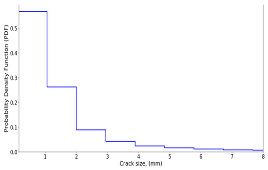
Figure 1.
Obtained prior crack size distribution by using the sampling method.
2.6. Estimation of Probability of Detection (POD)
Several fatigue cracks usually exist in a welded connection such as a tubular joint in the offshore platforms. Not all of these existing cracks can be detectable. The probability of detection of a crack depends on the resolution of the inspection technique. There is a wide variety of NDT techniques for finding cracks [23]. The probability of detection (POD), varies with crack size and the applied inspection technique. The probability of detection of a crack is usually given by [23]:
where amd, is the mean detectable size and it depends on the resolution of the inspection technique [23]. Figure 2 shows the POD curves for different mean detectable sizes.
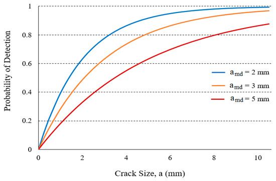
Figure 2.
Probability of detection (POD) curves for different mean detectable sizes.
In general, amd is an uncertain value, therefore in this study, a lognormal distribution (LN) is assigned to the prior estimation of the mean detectable size as:
Here, a large COV is considered for amd to have the prior as non-informative as possible. Non-informative priors are intended to let the data (observations) dominate the posterior distribution; thus, they contain little substantive information about the parameter of interest [24]. To find out which prior crack can be detected, Np random values of are selected based on the defined distribution.
2.7. Obtaining the Detected Cracks
In previous sections, Np simulations are performed for the crack size (ap) and also for the mean detectable size (). Therefore, for each crack size, a corresponding value of mean detectable size is available. In general, tiny cracks cannot be detected by using any NDT techniques. A criterion should be defined to show which prior crack size (with the corresponding ) is detectable and which one is missed. The proposed criterion is described below:
- (1)
- For each set of ; is calculated using Equation (13)
- (2)
- 105 random numbers are chosen from a uniform distribution between [0, 1], i.e.,:
- (3)
- (4)
- A prior crack size is assumed as a detected crack size if:
- (5)
- Otherwise, the simulated prior crack size is assumed as a missed one.
Figure 3 shows the detected and missed cracks based on the defined criterion. As the figure shows, the majority of the missed cracks are tiny defects, which are quite impossible to detect using NDT techniques.
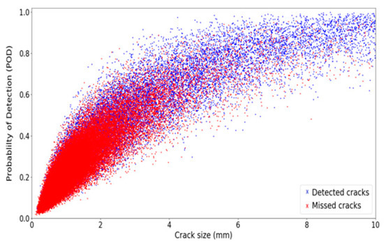
Figure 3.
Detected/missed cracks obtained by implementing the detection criterion.
3. Simulated Reality Estimations
It was demonstrated that the predicted crack size in a particular joint is a function of initial crack size, crack growth parameter, stress range, and geometry function. The assumed distributions of these input variables have a great impact on the crack size distribution [5,25]. Therefore, it is crucial to choose the most credible distributions for these parameters.
The accuracy of the reliability analysis results is dependent on the assumed distributions [25]. It was mentioned that the different recommended practices introduced various prior distributions for the uncertain parameters. However, these distributions are obtained based on experimental tests. Therefore, they are not representative of the real distributions. For example, the crack growth parameter is normally estimated by fitting fatigue test data measured under controlled, laboratory-environment conditions which are different from actual conditions in offshore platforms [2].
Since the real distributions for these uncertain parameters are unknown, in this study, an approach which is called the simulated reality distributions approach is used to obtain the real distributions. This approach is based on the concept of the equivalent initial flaw size.
3.1. Concept of Equivalent Initial Flaw Size
In the reliability analysis of aircraft structures, the initial crack size distribution plays a critical role in the distribution of the crack size [26]. To obtain the initial crack size distribution, Gray and Rudd [26] introduced the concept of equivalent initial flaw size (EIFS). This concept was developed for probabilistic risk analysis of aircraft by Yang and Manning [27].
The EIFS distribution is usually obtained by back extrapolating of the observed crack size to its corresponding size at time zero. This involves fitting a crack growth model to the crack size. Therefore, the EIFS is an artificial crack size [26] and for an observed crack size, the EIFS is not unique, i.e., for the same observed crack sizes, different EIFS values can be achieved by using different crack growth models [26]. Despite this shortcoming, the concept of the EIFS has been used to quantify the initial crack size distributions, due to its consistency with the crack growth to calculate the crack size at a given time [26].
For a given set of crack sizes (for a particular joint at different times), the equivalent initial flaw size (EIFS) distributions with the corresponding crack growth curves can be obtained as follows:
- (1)
- A specific crack size is selected as a baseline crack size ()
- (2)
- For a given set of crack sizes, the crack sizes that are bigger than the baseline crack size are regressed using the crack growth curve. Moreover, the crack sizes that are smaller than the baseline crack size are grown using the crack growth curve.
- (3)
- A probability density function (PDF) is assigned to the time that cracks reach the size of.
- (4)
- The time distribution of the baseline crack size is transferred to an initial crack size with a cumulative probability of.
- (5)
- Finally, an appropriate distribution for the equivalent initial flaw size (EIFS) is obtained.
- (6)
- Figure 4 illustrates the method for obtaining EIFS distribution.
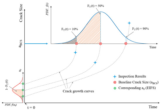 Figure 4. Obtaining the equivalent initial flaw size (EIFS) distribution.
The EIFS distribution is determined by regressing the observed crack sizes from inspection results back to the beginning of its fatigue life [27]. However, to obtain a suitable distribution, a sufficient number of data points are required, although the inspection data can be very limited and expensive to obtain. Therefore, the quality of the EIFS distribution depends on the number of available inspection results [27].
In the literature, the EIFS approach was considered to obtain the initial crack size distribution of aircraft. However, for the reliability analysis of offshore platforms, the distribution of the crack size at any given time depends on several uncertain parameters as presented in Equation (9). Therefore, in this study, the EIFS approach is extended for obtaining the equivalent distribution for all uncertain parameters affecting the crack size in a tubular joint.
3.2. Simulated Reality Distributions for Uncertain Parameters
Fatigue inspection results only include information about the crack sizes. Since the inspection cannot provide any explicit information about the other uncertain parameters, the distributions of these parameters are unknown. For this purpose, the concept of equivalent distributions is used for predicting the distribution of these parameters in the simulated reality.
To demonstrate the considered approach, it is assumed that five inspection results are available for the considered tubular joint at different years. Table 2 shows the assumed inspection results.
Table 2.
Assumed inspection results for the considered tubular joint
To obtain the simulated reality distribution for the initial crack size, the baseline crack size is selected as . For the given crack sizes inTable 2, the crack sizes that are bigger than the 4 mm are regressed and the crack sizes that are smaller than the 4 mm are grown using the crack growth curve. Table 3 shows the time to reach to 4 mm for each crack.
Table 3.
Crack growth/regression.
The mean value and standard deviation of the last column in Table 3 are calculated equal to 4.9 mm and 1.87 mm. Therefore, the following lognormal distribution is considered for the distribution of the time that crack reaches to baseline crack size:
To obtain the simulated reality distribution for the initial crack size, the mean values of the crack growth parameter, stress range, and the geometry function are selected. A large number of random samples are generated for time (TS) based on Equation (15) and for each sample, the corresponding initial crack size is obtained by using Equation (9).
Figure 5 shows how the equivalent initial crack size distribution is obtained by using the proposed approach for three randomly-generated times, schematically.
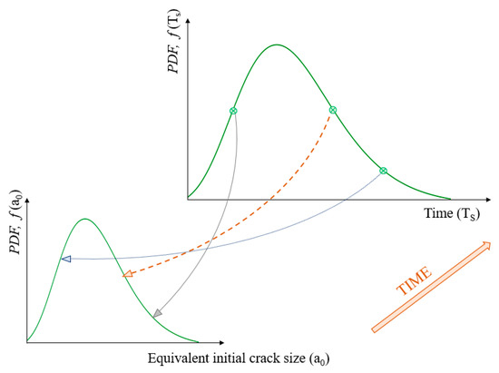
Figure 5.
Obtaining the equivalent initial crack size distribution.
Having obtained the initial crack size for each sample, the best distribution is fitted for the equivalent initial crack size histogram. Figure 6 illustrates the obtained equivalent initial crack size distribution for the considered tubular joint.
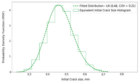
Figure 6.
Equivalent initial crack size histogram and the fitted distribution.
The same approach is utilized to derive the equivalent distribution for the crack growth parameter (C). Again, a large number of randomly generated samples for time (TS) is selected based on the lognormal distribution. To obtain the simulated reality distribution for the crack growth parameter, the mean values of the crack initial crack size, stress range, and the geometry function are selected. Figure 7 shows how the equivalent crack growth parameter distribution is obtained by using the proposed approach.
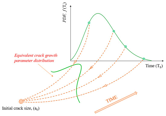
Figure 7.
Obtaining the equivalent crack growth parameter distribution.
Having obtained the crack growth parameter value for each sample, the best distribution is fitted for the equivalent crack growth parameter distribution. Figure 8 illustrates the obtained equivalent crack growth parameter distribution for the considered tubular joint.
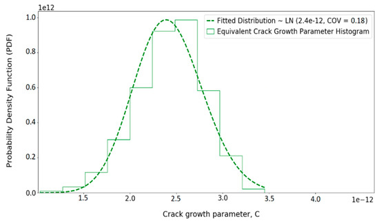
Figure 8.
Equivalent crack growth parameter histogram and the fitted distribution.
A similar approach is employed to obtain the equivalent distribution for the stress range and the geometry function. Figure 9 and Figure 10 show the obtained equivalent distributions for the stress range and the geometry function, respectively.
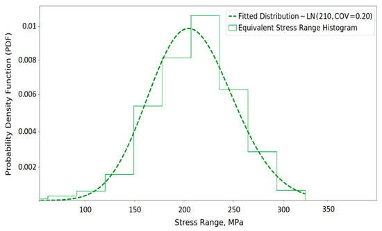
Figure 9.
Equivalent stress range histogram and the fitted distribution.
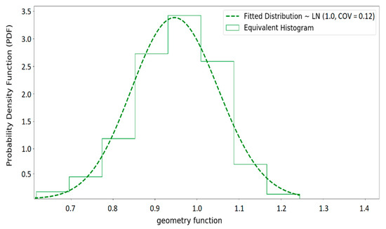
Figure 10.
Equivalent geometry function histogram and the fitted distribution.
Table 4 summarizes the obtained equivalent distributions for the uncertain parameters which are assumed as the real distributions. Since these distributions are achieved based on sampling methods, in this paper, they are called simulated reality distributions.
Table 4.
Simulated reality distributions for the uncertain parameters
3.3. Simulated Reality Distribution for Crack Size
Having obtained the simulated reality distributions for the input variables, the simulated reality distribution of the crack size can be obtained. Again, a sampling method is used to obtain the simulated reality distribution for the crack sizes after five years. For this purpose, random numbers are generated for each input variable based on their distributions presented in Table 4. For each set of samples (e.g., for the kth sample set: and), the crack size () is calculated based on Equation (9). Figure 11 shows the normalized histogram of the simulated reality crack sizes after five years which is used as a simulated reality distribution for the crack size.
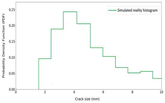
Figure 11.
Simulated reality distribution for the crack size.
It is noted that, in practice, only few inspection results are available for each tubular joint due to the expensive cost of the inspection. In the proposed sampling method, instead of using a few inspection results, a large number of artificial crack sizes that are generated based on inspection results are used. These generated cracks can be used for improving the distribution of uncertain parameters.
3.4. Simulated Reality Distribution for POD Curve
It was mentioned that the probability of detection of a crack depends on the resolution of the inspection technique. Here, a lognormal distribution with a mean value of 2 mm and coefficient of variation (COV) of 0.2 is considered for the simulated reality distribution of the mean detectable size as:
To find out which simulated reality crack can be detected, random values of are selected based on the defined lognormal distribution in Equation (16).
3.5. Obtaining the Detected Simulated Reality Cracks
In previous sections, 1000 crack sizes () and 1000 mean detectable size () are generated. Therefore, for each crack size, a corresponding value of mean detectable size is available. Some of the generated cracks in the sampling method are tiny. Therefore, they cannot be detected by using any NDT techniques. This approach is intended to use those cracks that can be detected.
The same criterion as in Section 2.7 is used to decide which crack size (with the corresponding ) is detectable and which one is missed. Figure 12 shows both detected and missed cracks.
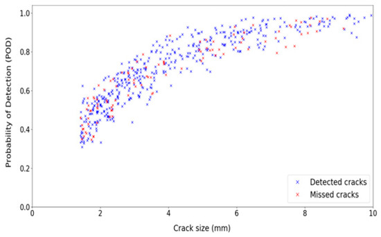
Figure 12.
Detected/missed cracks obtained by implementing the detection criterion.
4. Posterior Distributions of the Uncertain Parameters
Now, there are two sets of cracks; detected prior cracks and detected simulated reality cracks. to obtain the posterior distribution, each detected prior crack is compared with the simulated reality cracks to determine if the detected prior crack is compatible with reality. If the prior crack is ‘close’ to the simulated reality crack, that prior crack is assumed as a compatible simulation. The prior crack is considered as a compatible simulation if the following condition is satisfied:
with
where and represent the detected prior crack size and detected simulated reality crack size, respectively. The parameters zp and zr represent the number of detected prior crack and simulated reality cracks, respectively.
To quantify the word ‘close’, the parameter T is considered to represent the acceptable tolerance. If a small value is selected for tolerance, the difference between the prior crack and the simulated reality crack should be small. On the other hand, big value for tolerance allows a bigger difference between prior and the simulated reality cracks. Figure 13 shows the acceptable range for a prior crack for two different tolerances. To demonstrate the methodology, in this study, the parameter T is assumed equals to 0.2.
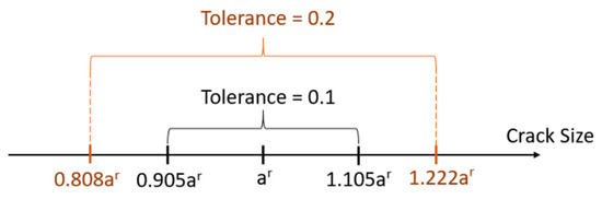
Figure 13.
The acceptable ranges for the prior cracks.
Based on the compatibility definition in Equation (17), many prior simulations may not match any real case. However, some prior simulations may match several real cases. By using Equation (17), the prior cracks are split into two categories; compatible priors and incompatible priors. For obtaining the posterior distribution, the incompatible prior simulations are removed and the compatible prior simulations are considered as the posterior cracks. In fact, by implementing this approach, the new data (which are simulated reality cracks) is utilized to improve the prior cracks and to obtain the posterior distribution of the crack sizes.
4.1. Updating the Crack Size Distribution
Figure 14 shows the posterior distribution of crack sizes that are obtained based on the compatible priors. Although both detected prior cracks and detected simulated reality cracks affect the posterior distribution shape, it is observed that the posterior distribution has moved towards the simulated reality distribution.
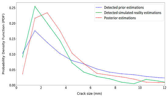
Figure 14.
Crack size distributions before and after updating.
It is also observed that the posterior distribution is narrower than the prior distribution. Therefore, the uncertainty of the posterior distribution for the crack size is reduced in comparison with the prior distribution. In fact, by implementing the inspection results, the posterior distribution for the crack size becomes less uncertain than the prior knowledge.
4.2. Updating the POD Curve
By removing the incompatible prior cracks, the posterior POD curve can be achieved. Figure 15a shows compatible prior simulation results and the fitted distribution. As can be seen from Figure 15b the posterior POD has moved towards the simulated reality data.
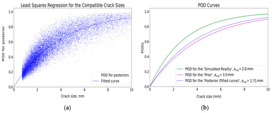
Figure 15.
Updating the POD curve based on the compatible simulations: (a) Compatible prior simulation results; (b) Fitted POD curve.
4.3. Updating the Distributions of Other Uncertain Parameters
If a specific detected prior crack, is incompatible, it means that the combination of the corresponding input variables (and) are not producing an acceptable prior crack size. Therefore, these values (and) are removed from the initial set of prior simulations. On the other hand, if a simulated prior crack is a compatible crack size with the simulated reality, the corresponding input variables are appropriate values and they are kept to use for the posterior distributions.
Figure 16, Figure 17, Figure 18 and Figure 19 show the posterior distributions for the uncertain input variables. Similar to Figure 14, the posterior distributions of the uncertain parameters have moved towards the simulated reality distribution. For example, in Figure 17, when the crack growth parameter is around, the posterior distribution is ascending and the prior distribution is descending. The figure illustrates that the posterior distribution tends to shift towards the simulated reality distribution.
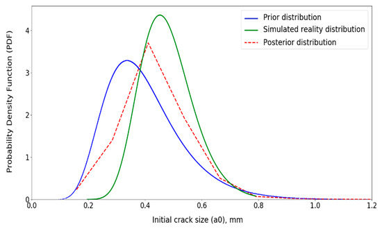
Figure 16.
Updated distribution for initial crack size ().
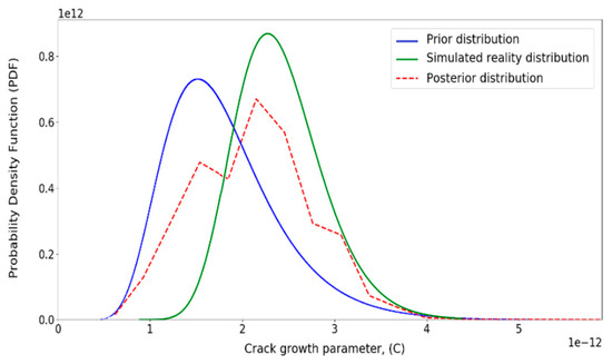
Figure 17.
Updated distribution for crack growth parameter (C).
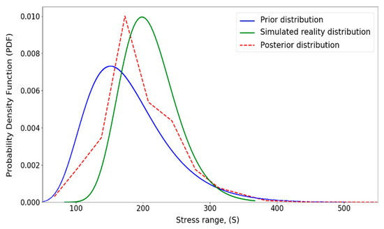
Figure 18.
Updated distribution for stress range (S).
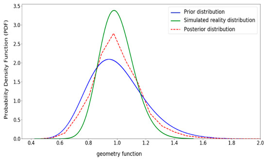
Figure 19.
Updated distribution for geometry function (Y).
Moreover, in these figures, the most probable amount of the random variable (mode value) is shifted towards the mode value of the simulated reality distributions. It is worth mentioning that the shape of the posterior distribution is affected by both prior and simulated reality distributions.
The updated distributions can be used as the prior distributions for the next updating process when new inspection results are available. Therefore, for the next updating process, instead of using generalized distributions provided by recommended practices, more realistic distributions can be selected as prior distributions.
It is found in Figure 14, that the uncertainty of the posterior crack size distribution decreases. However, it is observed that the uncertainty of the posterior distributions of the other parameters increases due to the involved uncertainties in both prior and simulated reality distributions. The reason is that the inspection results include only the crack size information and they do not provide any explicit information about the other parameters.
Although the uncertainty of the posterior distributions of the input variables increases, the prior distributions of the input variables are modified based on the real situation of the considered tubular joint. It was mentioned that the prior distributions are based on experimental tests that are different from the real condition of the platform. Therefore, for the next updating process (when these posterior distributions are considered as the prior distributions for updating), the prior distributions are more reliable than the introduced distributions in the recommended practices and the uncertainties will be gradually reduced during the next updating process.
5. Conclusions
In this study, a methodology is presented to update the probability distribution of uncertain parameters when new information (inspection results) becomes available. Such information can be used to update the probability distributions of the uncertain parameters. Crack size, POD curve, initial crack size, crack growth parameter, stress range, and geometry function are considered as uncertain parameters.
The fatigue probability of failure of tubular joints depends on the crack size distribution. Since the crack size is a function of several parameters, the distributions of these parameters affect the crack size distribution. Different studies suggest various distributions for these parameters. Therefore, the selection of the appropriate prior distributions is crucial and sometimes difficult. In this study, a framework is developed to improve the prior knowledge about the uncertain parameters. Moreover, the framework is capable to update the crack size distribution and the probability of failure.
The proposed methodology utilizes the simulated reality data to understand how the prior assumptions combine with observations to improve the posterior estimates from the Bayesian procedure. In this study, simulated reality data is used, rather than real data, because there will not usually be sufficient real data to check the behavior of the method.
The sampling method is used to generate the prior distribution of crack sizes. A large number of random numbers for each input variable are generated based on their distributions. The crack size is then calculated for each set of randomly generated samples. Moreover, to obtain the simulated reality distributions of the input variables, the concept of equivalent initial flaw size distribution is utilized. For obtaining the posterior distribution, the concept of compatibility is defined. For this purpose, each detected prior crack is compared with each simulated reality crack. If the prior crack is close to the simulated reality, it is assumed as a compatible prior otherwise it is considered as an incompatible prior. The posterior distribution is then achieved by removing the incompatible priors and fitting the best distribution to the compatible priors.
The results of this updating method show that the posterior distributions of uncertain parameters shift toward to the simulated reality distribution. It is also shown that the uncertainty of the posterior crack size distribution decreases whereas the uncertainty of input variables increases since the inspection results include only data about the crack size and do not provide any information about the input variables.
The updated distributions will be used as the prior distributions for the next updating process when new inspection results are available.
Author Contributions
The methodology was developed by H.K. and N.B. together with S.O. and U.B. H.K. performed the numerical simulation. The paper was written by H.K. and S.O. and it was reviewed by S.O., N.B., and U.B. All authors have read and agreed to the published version of the manuscript.
Funding
This research was funded by the sponsorship and support of Lloyd’s Register Foundation.
Acknowledgments
This publication was made possible by the sponsorship and support of Lloyd’s Register Foundation. The Foundation helps to protect life and property by supporting engineering-related education, public engagement, and the application of research. The work was enabled through, and undertaken at, the National Structural Integrity Research Centre (NSIRC), a postgraduate engineering facility for industry-led research into structural integrity established and managed by TWI through a network of both national and international Universities.
Conflicts of Interest
The authors declare no conflict of interest.
References
- Heredia-Zavoni, E.; Montes-Iturrizaga, R. A Bayesian Model for the Probability Distribution of Fatigue. J. Offshore Mech. Arct. Eng. 2004, 126, 243–249. [Google Scholar] [CrossRef]
- Karandikar, J.M.; Kim, N.H.; Schmitz, T.L. Prediction of remaining useful life for fatigue-damaged structures using Bayesian inference. Eng. Fract. Mech. J. 2012, 96, 588–605. [Google Scholar] [CrossRef]
- Peng, T.; He, J.; Xiang, Y.; Liu, Y.; Saxena, A.; Celaya, J.; Goebel, K. Probabilistic fatigue damage prognosis of lap joint using Bayesian updating. J. Intell. Mater. Syst. Struct. 2015, 26, 965–979. [Google Scholar] [CrossRef]
- Carr, P.; Busby, P.L.; Cresswell, S.M. A Unified Probabilistic Approach to Design & Inspection of Offshore Steel Structures. In Proceedings of the Third International Symposium on Integrity of Offshore Structures, Glasgow, UK, 28–29 September 1987; pp. 375–394. [Google Scholar]
- DNV. Guideline for Structural Reliability Analysis: Application to Jacket Platforms; Report No. 95-3203; DNV: HØVIK, Norway, 1995. [Google Scholar]
- JCSS. Fatigue Models for Metallic Structures; Joint Committee on Structural Safety: Aalborg, Denmark, 2011. [Google Scholar]
- Siddiqui, N.A.; Ahmad, S. Fatigue and fracture reliability of TLP tethers under random loading. Mar. Struct. 2001, 14, 331–352. [Google Scholar] [CrossRef]
- Gelman, A.; Carlin, J.B.; Stern, H.S.; Rubin, D.B. Bayesian Data Analysis, 2nd ed.; Chapman and Hall/CRC Press: New York, NY, USA, 2009. [Google Scholar]
- Aghakouchak, A.A.; Stiemer, S.F. Fatigue reliability assessment of tubular joints of existing offshore structures. Can. J. Civ. Eng. 2001, 28, 691–698. [Google Scholar] [CrossRef]
- Almar-Naess, A. Fatigue Handbook for Offshore Steel; Tapir Publication: Trondheim, Norway, 1985. [Google Scholar]
- Etube, L.S. Fatigue and Fracture Mechanics of Offshore Structures; Professional Engineering Publishing Limited: London, UK, 2001. [Google Scholar]
- Dover, W.D.; Dharmavasan, S. Fatigue and Fracture Mechanics Analysis of T and Y joints. In Proceedings of the Offshore Technology Conference, OTC 4404, Houston, TX, USA, 3–6 May 1982. [Google Scholar]
- Lee, M.M.K.; Bowness, D. Stress intensity factors for weld toe cracks in tubular joints. In Proceedings of the Fifth International Conference on Engineering Structural Integrity Assessment, Cambridge, UK, 19–21 September 2000. [Google Scholar]
- He, J.; Yang, J.; Wang, Y.; Waisman, H.; Zhang, W. Probabilistic Model Updating for Sizing of Hole-Edge Crack Using Fiber Bragg Grating Sensors and the High-Order Extended Finite Element Method. Sensors 2016, 16, 1956. [Google Scholar] [CrossRef] [PubMed]
- DNV-GL SESAM Genie; V 7.4; Det Norske Veritas Software: Oslo, Norway, 2015.
- Wirshing, P.H.; Light, M.C. Fatigue under wide band random stresses. ASCE J. Struct. Div. 1980, 106, 1593–1607. [Google Scholar]
- Karadeniz, H. Uncertainty Modelling in the Fatigue Reliability Calculation of Offshore Structures. Reliab. Eng. Syst. Saf. 2001, 74, 323–335. [Google Scholar] [CrossRef]
- BS 7910:2013. Guide to Methods of Assessing the Acceptability of Flaws in Metallic Structures, 3rd ed.; BSI: London, UK, December 2013. [Google Scholar]
- Khalili, H.; Oterkus, S.; Barltrop, N.; Bharadwaj, U.; Tipping, M. System reliability calculation of jacket platforms including fatigue and extreme wave loading. Trends in the Analysis and Design of Marine Structures. In Proceedings of the 7th International Conference on Marine Structures, Marstruct, Dubrovnik, Croatia, 6–8 May 2019; Taylor & Francis Group: London, UK, 2015. [Google Scholar]
- Lin, H.; Chen, G.; Wang, Z.; Yang, L. Integrality Assessment of Tubular Joints in Aging Offshore Platform Based on Reliability Theory. Adv. Mater. Res. 2012, 532–533, 238–242. [Google Scholar] [CrossRef]
- Val, D. Safety, Risk and Reliability; Heriot-Watt University: Edinburgh, UK, 2014. [Google Scholar]
- Python V.3.7. Available online: www.python.org (accessed on 3 October 2020).
- Moan, T. Reliability-based management of inspection, maintenance, and repair of offshore structures. Struct. Infrastruct Eng. 2005, 1, 33–62. [Google Scholar] [CrossRef]
- Kelly, D.; Smith, C. Bayesian Inference for Probabilistic Risk Assessment; Springer: Idaho Falls, ID, USA, 2011. [Google Scholar]
- Rajasankar, J.; Iyer, N.R.; Appa Rao, T.V.S.R. Structural integrity assessment of offshore tubular joints based on reliability analysis. Int. J. Fatigue 2003, 25, 609–619. [Google Scholar] [CrossRef]
- Rudd, J.L.; Gray, T.D. Quantification of fastener-hole quality. J. Aircr. 1978, 15, 143–147. [Google Scholar] [CrossRef]
- Yang, J.N.; Manning, S.D. Statistical distribution of equivalent initial flaw size. In Proceedings of the Annual Reliability and Maintainability Symposium, San Francisco, CA, USA, 22–24 January 1980. [Google Scholar]


© 2020 by the authors. Licensee MDPI, Basel, Switzerland. This article is an open access article distributed under the terms and conditions of the Creative Commons Attribution (CC BY) license (http://creativecommons.org/licenses/by/4.0/).