An Explicit Algebraic Closure for Passive Scalar-Flux: Applications in Channel Flows at a Wide Range of Reynolds Numbers

Abstract

In this paper, we propose an algebraic model for turbulent scalar-flux vector that stems from tensor representation theory. The resulting closure contains direct dependence on mean velocity gradients and quadratic products of the Reynolds stress tensor. Model coefficients are determined from Direct Numerical Simulations (DNS) data of homogeneous shear flows subjected to arbitrary mean scalar gradient orientations, while a correction function was applied at one model coefficient based on a turbulent channel flow case. Model performance is evaluated in Poiseuille and Couette flows at several Reynolds numbers for $Pr=0.7$, along with a case at a higher Prandtl number ($Pr=7.0$) that typically occurs in water–boundary interaction applications. Overall, the proposed model provides promising results for wide near-wall interaction applications. To put the performance of the proposed model into context, we compare with Younis algebraic model, which is known to provide reasonable predictions for several engineering flows.

1. Introduction

Reynolds-Averaged Navier–Stokes (RANS) and Large Eddy Simulations (LES) approaches are today widely used in engineering applications for predicting the dynamics and scalar transfer of turbulent flows. Both approaches have existed for a long time and will remain useful for understanding several industrial configurations for several decades, playing different roles. In a LES, the larger scales in a flow are computed explicitly, but the effect of the smaller unresolved scales is modeled. The basic ingredient of LES modeling is a model for the sub-grid dynamics in terms of the resolved velocity field: a so-called eddy-viscosity model. An important example of an eddy-viscosity model for LES is the classical Smagorinsky model [1]. The Smagorinsky model gives good results for homogeneous isotropic turbulence, but removes too much kinetic energy from laminar and transitional flows. Minimum-dissipation eddy-viscosity models are a class of sub-filter models for large-eddy simulation that give the minimum eddy dissipation required to dissipate the energy of sub-filter scales. A class of minimum-dissipation that has many desirable properties is the QR model [2]. In particular, this model is based on the invariants of the resolved rate-of-strain tensor, it appropriately switches off for laminar and transitional flows, has low computational complexity, and is consistent with the exact sub-filter tensor on isotropic grids. A generalization of the QR model to anisotropic grids, called anisotropic minimum-dissipation (AMD) model, has been also proposed, which also does not require an approximation of the filter width [3]. Another subgrid-scale stress model that is economical in adding eddy dissipation is Nicoud’s sigma models [4]. This closure has the elegant property to automatically vanish as soon as the resolved field is either two-dimensional or two-component, including the pure shear and solid rotation cases. Further considerations on minimizing eddy viscosity by means of invariants can be found in [5,6], whereas a good summary of low-dissipation models can be found in Rozema et al. [7].

An alternative way of modeling turbulence is by means of Reynolds averaging the Navier–Stokes equations. In contrast to LES, in RANS all turbulent flow scales are being modeled. The present study focuses on developing a RANS-based model for the turbulent scalar-flux vector. Turbulent scalar-flux vector appears in the Reynolds-averaged scalar transport equations as a term that needs to be modeled so that closure is achieved. An elegant choice is the development of engineering models with aim to provide estimations of this quantity at low computational complexity. Engineering models for the scalar-flux are classified into two categories: differential and algebraic. Differential transport models (DTM) are proven to be beneficial tools, being capable of handling rotational and curvature effects. However, robustness issues and performance inconsistencies, combined with computational overheads associated with the solution of a differential transport equation for each scalar-flux component, prevent this class of models from penetrating further into the mainstream of engineering practice. On the other hand, algebraic approaches are based on assumptions that lead to constitutive equations between turbulent statistics and mean deformation. The simplest algebraic model is based on the gradient diffusion hypothesis (GDH), which assumes that turbulent scalar-flux is aligned to the mean scalar gradient. Despite its implementational and computational elegance, this assumption is an important reason why this model fails to capture important flow features, such as turbulence anisotropy or the effects of mean and system rotation. As a result, [8] proposed a generalization of GDH (GGDH) from which several algebraic closures have emerged. For example, [9] adopted scale functions to express the turbulent scalar-flux vector as a product between Reynolds stress and mean scalar-gradient, allowing the misalignment of the scalar-fluxes with the mean scalar deformation. However, this expression is found to perform poorly on predicting the correct magnitudes of scalar-flux components in the directions normal to the mean scalar gradient. [10] improved the performance of the GGDH model by adding a nonlinear term that contains quadratic products of the Reynolds stress tensor, which correctly captures the inclination levels of the scalar-flux components in the vicinity of wall boundaries. This addition resulted in the construction of Higher-Order GGDH models (HO-GGDH), which were successfully applied in a wide range of channel flows. Another interesting approach is to derive algebraic expressions directly from the exact transport equation of turbulent scalar-flux through equilibrium assumptions. A common choice is to apply the weak-equilibrium assumption (WEA), proposed in [11], which states that the transient variations of turbulent anisotropies are negligible compared to the variation of turbulent scales. To some extent, these models are considered to be a good alternative to DTM, as they have been successfully applied in different flow configurations while requiring less computational capacity [12,13,14].

An alternative approach for estimating the turbulent scalar-fluxes was proposed by [15]. Using as guidance the exact scalar-flux transport equation, Younis and coworkers expressed this quantity as a function of several tensor quantities. This approach is elegant, as it avoids the reduction of transport equations through the WEA with all the modeling uncertainties that entails. It also provides a general framework, from which different algebraic expressions can be obtained. They proposed a multi-linear closure that exhibited distinct improvements over other algebraic scalar-flux closures for benchmark cases, for example two-dimensional free shear flows and configurations involving curvature effects ([16]). However, the linear nature of this specific closure is the main reason why it fails to capture the proper near-wall misalignment levels of scalar-flux vector, thus revealing the importance of incorporating nonlinear information regarding turbulence anisotropy. Therefore, in this study we propose an algebraic model that stems directly from the Younis formulation and involves products of the Reynolds stress tensor, a dependence missing from the multi-linear model. Special attention is given so that model complexity is kept minimal for ease implementation in existing industrial codes, while its performance ability is tested on several Couette and Poiseuille flows at a wide range of Reynolds numbers and a Prandtl number equal to 0.7 and 7.0. The former $Pr$ number is encountered in aerodynamic applications, whereas the latter number typically occurs in marine applications and water-boundary interaction.

A description of the exact transport equations of the turbulent passive-scalar fluxes along with an extensive summary of the Younis approach are given in Section 2 with the motivation behind the use of a nonlinear term involving products of Reynolds stress given in Section 3. The proposed formulation is discussed in Section 4 and the performance of this closure is evaluated in Section 5, yielding encouraging results. Summary and conclusions are given in Section 6.

2. Younis’ Formulation

The motivation behind the work reported by [15] arose from the need to provide a better alternative to the existing gradient-transport closures for the turbulent scalar-fluxes. As a starting point, they considered the exact transport equation of the following fluxes,

$$\begin{array}{cc}\hfill \frac{\partial \overline{u_i^{\prime }{\varphi }^{\prime }}}{\partial t}+{\overline{u}}_j\frac{\partial \overline{u_i^{\prime }{\varphi }^{\prime }}}{\partial x_j}=& -\overline{u_i^{\prime }{u}_j^{\prime }}\frac{\partial \overline{\varphi }}{\partial x_j}-\overline{u_j^{\prime }{\varphi }^{\prime }}\frac{\partial {\overline{u}}_i}{\partial x_j}-(\gamma +\nu )\overline{\frac{\partial {\varphi }^{\prime }}{\partial x_j}\frac{\partial u_i^{\prime }}{\partial x_j}}\hfill \\ \hfill & -\frac{1}{\rho }\overline{p^{\prime }\frac{\partial {\varphi }^{\prime }}{\partial x_i}}-\frac{\partial }{\partial x_j}\left(\overline{u_i^{\prime }{u}_j^{\prime }{\varphi }^{\prime }}+\frac{1}{\rho }\overline{p^{\prime }{\varphi }^{\prime }}{\delta }_{ij}-\gamma \overline{u_i^{\prime }\frac{\partial {\varphi }^{\prime }}{\partial x_j}}-\nu \overline{{\varphi }^{\prime }\frac{\partial u_i^{\prime }}{\partial x_j}}\right),\hfill \end{array}$$

(1)

where the instantaneous flow variables are decomposed into a mean part, denoted by overbar, and a fluctuating part, denoted by prime symbol. Hereafter, we are using index notation whereby repeated indexes imply summation. The coefficient of fluid viscosity and the coefficient of scalar diffusivity are denoted by $\nu$ and $\gamma$, respectively, $\rho$ is the density of the fluid and $u_i$, $\varphi$ are the instantaneous fluid velocity and passive scalar fields, respectively. The fluctuating pressure is denoted with $p^{\prime }$. The first and second terms on the RHS of Equation (1) represent the generation of scalar-flux as a consequence of turbulence-mean deformation interactions. The third term refers to the rate at which the scalar-flux is destructed, while the fourth term refers to the fluctuating pressure-scalar correlations and is responsible for the redistribution of the flux among the different components. The last term is interpreted as the turbulent-transport term. [15] used Equation (1) as a guide to provide a rationally assumed relationship between the scalar-flux vector and various tensor quantities,

$$\overline{u_i^{\prime }{\varphi }^{\prime }}=f_i\left(R_{ij},S_{ij},{\mathsf{\Omega }}_{ij},{\mathsf{\Lambda }}_i,ϵ,{ϵ}_{\varphi },\overline{{\varphi }^{{}^{\prime }2}}\right),$$

(2)

where $R_{ij}=\overline{u_i^{\prime }{u}_j^{\prime }}$ is the Reynolds stress tensor, $ϵ$ is the energy dissipation rate, ${ϵ}_{\varphi }$ is half the scalar dissipation rate, and $\overline{{\varphi }^{{}^{\prime }2}}$ is the scalar-variance. $S_{ij}$, ${\mathsf{\Omega }}_{ij}$, and ${\mathsf{\Lambda }}_i$ denote the mean strain rate tensor, the mean vorticity tensor, and the mean scalar gradient vector, respectively, defined as

$$\begin{array}{cc}\hfill S_{ij}& =\frac{1}{2}\left(\frac{\partial {\overline{u}}_i}{\partial x_j}+\frac{\partial {\overline{u}}_j}{\partial x_i}\right),{\mathsf{\Omega }}_{ij}=\frac{1}{2}\left(\frac{\partial {\overline{u}}_i}{\partial x_j}-\frac{\partial {\overline{u}}_j}{\partial x_i}\right),{\mathsf{\Lambda }}_i=\frac{\partial \overline{\varphi }}{\partial x_i}.\hfill \end{array}$$

(3)

With the aid of tensor representation theory, Younis et al. constructed an explicit model for $\overline{u_i^{\prime }{\varphi }^{\prime }}$ in accordance with Equation (2). Under this approach, $\overline{u_i^{\prime }{\varphi }^{\prime }}$ can be expressed as a series of basis vectors ${\mathrm{Y}}_i$,

$$\overline{u_i^{\prime }{\varphi }^{\prime }}={\displaystyle \sum _{n=1}^M}{\alpha }_n{\mathrm{Y}}_i^n,$$

(4)

where ${\alpha }_n$ can depend on all the tensor variables appearing in Equation (2). The basis vectors are formed from the products of the symmetric ($S_{ij},R_{ij}$), the skew-symmetric (${\mathsf{\Omega }}_{ij}$) tensor and the vector (${\mathsf{\Lambda }}_i$), leading to the following algebraic expression.

$$\begin{array}{cc}\hfill \overline{u_i^{\prime }{\varphi }^{\prime }}& ={\alpha }_1{\mathsf{\Lambda }}_i+{\alpha }_2{R}_{ij}{\mathsf{\Lambda }}_j+{\alpha }_3{S}_{ij}{\mathsf{\Lambda }}_j+{\alpha }_4{R}_{ik}{R}_{kj}{\mathsf{\Lambda }}_j+{\alpha }_5{S}_{ik}{S}_{kj}{\mathsf{\Lambda }}_j+{\alpha }_6{\mathsf{\Omega }}_{ij}{\mathsf{\Lambda }}_j\hfill \\ \hfill & +{\alpha }_7{\mathsf{\Omega }}_{ik}{\mathsf{\Omega }}_{kj}{\mathsf{\Lambda }}_j+{\alpha }_8\left(S_{ik}{\mathsf{\Omega }}_{kj}+S_{jk}{\mathsf{\Omega }}_{ki}\right){\mathsf{\Lambda }}_j+{\alpha }_9\left(R_{ik}{S}_{kj}+R_{jk}{S}_{ki}\right){\mathsf{\Lambda }}_j\hfill \\ \hfill & +{\alpha }_{10}\left(R_{ik}{\mathsf{\Omega }}_{kj}+R_{jk}{\mathsf{\Omega }}_{ki}\right){\mathsf{\Lambda }}_j.\hfill \end{array}$$

(5)

To bring the above expression into a more compact form, [15] assumed sufficiently small anisotropies and turbulent time scales. Further assuming that the effects of $S_{ij}$ and ${\mathsf{\Omega }}_{ij}$ are in balance, results to the following multi-linear expression,

$$\begin{array}{cc}\hfill \overline{u_i^{\prime }{\varphi }^{\prime }}& =C_1\frac{{\kappa }^2}{ϵ}{\mathsf{\Lambda }}_i+C_2\frac{\kappa }{ϵ}{R}_{ij}{\mathsf{\Lambda }}_j+C_3\frac{{\kappa }^3}{{ϵ}^2}{G}_{ij}{\mathsf{\Lambda }}_j+C_4\frac{{\kappa }^2}{{ϵ}^2}\left(R_{ik}{G}_{jk}+R_{jk}{G}_{ik}\right){\mathsf{\Lambda }}_j,\hfill \\ \hfill G_{ij}& =S_{ij}+{\mathsf{\Omega }}_{ij},\hfill \end{array}$$

(6)

where $\kappa =R_{kk}/2$ is the turbulent kinetic energy, while the ${\alpha }_i$ coefficients were replaced based on dimensional arguments. The first term on the RHS of Equation (6) represents the GDH, while the second term coincides with the production term that appears in Equation (1) and is associated with the mean scalar deformation, also known as the Generalized Gradient Diffusion Hypothesis (GGDH) model proposed in [9]. The remaining two terms involve products between the gradients of mean scalar and mean velocity a dependence proposed by the analyses of the works in [17,18]. The values of $C_i$ coefficients were determined based on the LES results of [19] for homogeneous flows subjected to a uniform shear with uniform scalar gradients

$$C_1=0.0455,C_2=-0.373,C_3=0.00373,C_4=0.0235.$$

(7)

Regarding inhomogeneous flows, detailed analysis of the model performance in relation to data from a large number of studies on wall-bounded flows showed a serious error in the normal flux component [16]. For example, the normal component of (6) takes the following form for flat-wall flows

$$\overline{u_2^{\prime }{\varphi }^{\prime }}=(C_1\kappa +C_2{R}_{22})\frac{\kappa }{ϵ}{\mathsf{\Lambda }}_2.$$

(8)

Using DNS data [20] for a fully-developed turbulent channel flow, it can be seen that

$$C_1\kappa +C_2{R}_{22}>0,$$

(9)

near the wall ($0<y^{+}<24$). Using the above expression into Equation (8) incorrectly predicts that $\overline{u_2^{\prime }{\varphi }^{\prime }}$ and ${\mathsf{\Lambda }}_2$ have the same sign. As a result, the value of $C_1$ coefficient was modified in the near-wall region by applying the following damping function,

$$C_1=0.0455f_{C_1},f_{C1}=1-\exp (-A\beta P{e}^{\alpha }),Pe=PrR{e}_t,$$

(10)

where $\alpha =-0.02$ and $\beta =1.9$ are the values proposed in [21], $Pr=\nu /\gamma$ is the Prandtl number, $R{e}_t=\frac{{\kappa }^2}{\nu ϵ}$ is the turbulence Reynolds number, and A is the stress-flatness parameter, defined as

$$\begin{array}{cc}\hfill A_{ij}& =\frac{R_{ij}}{\kappa }-\frac{2}{3}{\delta }_{ij},A_2=A_{ij}{A}_{ji},A_3=A_{ij}{A}_{jk}{A}_{ki},\hfill \\ \hfill A& =1-\frac{9}{8}(A_2-A_3),\hfill \end{array}$$

(11)

where $A_2$ and $A_3$ are the second and third invariants of the normalized Reynolds-stress anisotropic tensor $A_{ij}$. More details regarding the mathematical formulation can be found in [16]. As already mentioned in the introduction, the linear form of Younis closure is an important reason why this closure exhibits certain limitations. For example, it fails to capture the near-wall relative magnitudes between the scalar-flux components. In the following section we discuss the importance of incorporating a term that contains nonlinear information regarding the turbulent anisotropy, vital to predict the proper near-wall behavior.

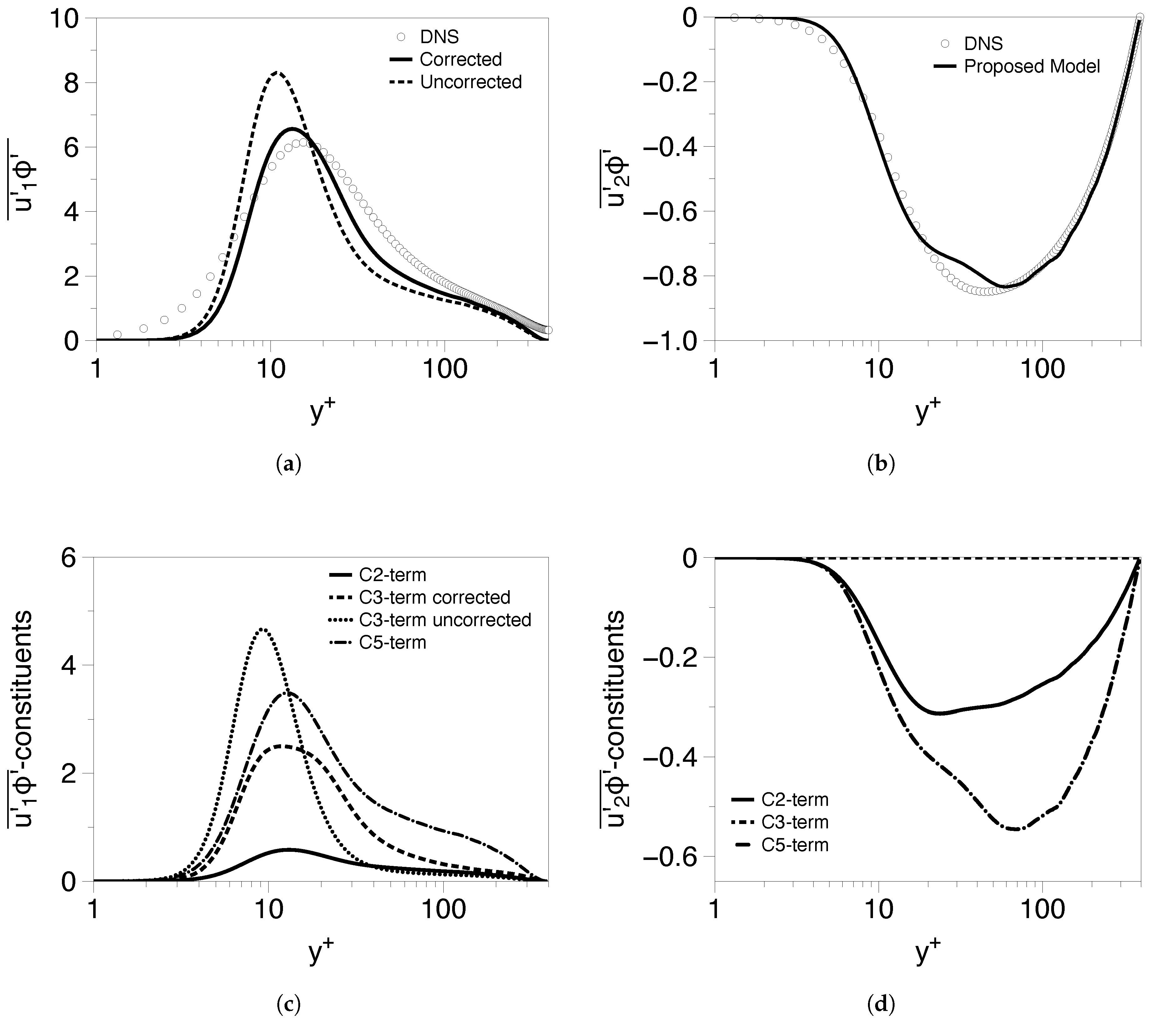
3. Quadratic Dependence on Reynolds Stress

It is well known that models involving only the second term of Equation (6) cannot predict the streamwise scalar-flux component reasonably well [22]. In an attempt to extend their applicability, [23] performed a series of LES simulations for fully developed turbulent channel flows under different boundary conditions and for a wide range of Prandtl numbers. They relied on the findings of [24], who pointed out that scalar fluctuations are correlated more strongly with streamwise than transverse velocity fluctuations in the near-wall region, to propose an algebraic relation between the turbulent scalar-flux vector and quadratic products of Reynolds stress tensor:

$$\overline{u_i^{\prime }{\varphi }^{\prime }}=-C_{\varphi }\tau \left(\frac{R_{ik}{R}_{kj}}{\kappa }\right){\mathsf{\Lambda }}_j,$$

(12)

where $\tau$ is a turbulent time scale and $C_{\varphi }$ is a model coefficient. In wall-bounded channel flows where statistical quantities are functions only of the wall-distance, the above expression approaches the following near-wall limit,

$$R_{u^{\prime }{\varphi }^{\prime }}\equiv \frac{\overline{u_2^{\prime }{\varphi }^{\prime }}}{\overline{u_1^{\prime }{\varphi }^{\prime }}}=\frac{R_{12}^2+R_{22}^2}{(R_{11}+R_{22})R_{12}}\to \frac{R_{12}}{R_{11}},$$

(13)

where subscripts 1, 2, and 3 are, respectively, the streamwise, wall-normal, and spanwise directions [23] also observed that the correlation between ${\varphi }^{\prime }$ and $u_2^{\prime }$ relatively increases with the decrease of $Pr$, reaching almost the same level as that between ${\varphi }^{\prime }$ and $u_1^{\prime }$ for $Pr=0.025$. As a result, they recommended that an effective algebraic scalar-flux model should depend both on linear and quadratic forms of Reynolds stress, written as

$$\overline{u_i^{\prime }{\varphi }^{\prime }}=-\kappa \tau \left(C_{\varphi ,1}\frac{R_{ij}}{\kappa }+C_{\varphi ,2}\frac{R_{ik}{R}_{kj}}{{\kappa }^2}\right){\mathsf{\Lambda }}_j,$$

(14)

where $C_{\varphi ,1}$ and $C_{\varphi ,2}$ are model coefficients. These coefficients should be determined so that the nonlinear term in Equation (14) becomes dominant in regions of high deformation rates, while the linear term becomes significant in the presence of weak strain rates, as well as in low Prandtl numbers. Hence, the present study aims to propose an algebraic model based on Younis general form (5) that involves the nonlinear term, and validate its performance in different channel flows.

4. Proposed Formulation

In this section, we introduce the proposed model, which is essentially a combination between the multi-linear model of Younis (6) and the functional form proposed by Abe and Suga (14), thus incorporating nonlinear information regarding turbulence anisotropy. Special attention is given to keep the model as simple as possible so that it can be easily implemented in existing industrial codes. This is achieved by investigating the contribution of each term appearing in the above equations in an attempt to propose a minimal combination of these terms that is able to provide reasonable predictions. We chose to neglect the $C_1$-related term by assuming that information regarding this term is partly included in the isotropic part of the second term of Equation (6). We have also excluded the term associated with $C_4$, even though its inclusion could provide additional flexibility, for the following reasons. First, this term cannot induce the proper near-wall anisotropy levels of the scalar-flux vector, as given in Equation (13). Second, this term involves products between the mean velocity gradients and the Reynolds stress, thus being more complex than the $C_3$-related term, which also contains gradients of the mean velocity field. Third, its absence facilitated our effort to apply minimal corrections to the model coefficients, as will be shown in this Section. Consequently, the proposed closure takes the following compact form,

$$\overline{u_i^{\prime }{\varphi }^{\prime }}=C_2\frac{\kappa }{ϵ}{R}_{ij}{\mathsf{\Lambda }}_j+C_3\frac{{\kappa }^3}{{ϵ}^2}{G}_{ij}{\mathsf{\Lambda }}_j+\frac{C_5}{ϵ}{R}_{ik}{R}_{kj}{\mathsf{\Lambda }}_j,$$

(15)

where we keep the same indexing for the model coefficients as in Equation (6). The above equation essentially differs from Equation (14) in involving the $C_3$-related term, which accounts for the products between mean scalar and mean velocity gradients.

4.1. Redistributive Term

In order to bring closure to the transport equations of the turbulent scalar-fluxes and stresses, it is required to model correlations that involve the fluctuating pressure $p^{\prime }$. As the action of the pressure interactions is known to redistribute the turbulent kinetic energy among the diagonal components of the Reynolds stresses, it is a common practice to re-express the pressure term that exist in the stress equations as the sum of a traceless distributive term, called the pressure–strain correlation, and the divergence of the correlation between the fluctuating velocity and the pressure field (added to the turbulent diffusion). As pressure is also present in the scalar equations, an analogous treatment has been employed that splits the pressure-related term in two parts: a correlation term $\overline{p^{\prime }\frac{\partial {\varphi }^{\prime }}{\partial x_i}}$ that redistributes the scalar-flux among its different components, and its divergence that is absorbed in the turbulent-transport term

$$\overline{\frac{1}{\rho }\overline{{\varphi }^{\prime }\frac{\partial p^{\prime }}{\partial x_i}}}=\frac{\partial }{\partial x_i}\left(\overline{\frac{p^{\prime }{\varphi }^{\prime }}{\rho }}\right)-\overline{p^{\prime }\frac{\partial {\varphi }^{\prime }}{\partial x_i}},$$

(16)

which explains the terms appearing at the RHS of (1). Given the level of approximation and empiricism that, inevitably, is needed in order to derive an algebraic model form, it is not possible to associate one particular term in the resulting algebraic expression (15) with the pressure-correlation term. Several models have been developed to model this term [25,26,27], suggesting that no consensus has been achieved regarding the modeling of this term. In an attempt to associate the terms appearing in the proposed closure (15) with the pressure-scalar correlation, we consider the elegant analysis conducted in [17], who represented the fluctuating parts of scalar and pressure as Fouries series in order to derive the following expression that relates pressure-correlation term with turbulent variables that appear in the transport equation

$$\begin{array}{cc}\hfill \frac{1}{\rho }\overline{p^{\prime }\frac{\partial {\varphi }^{\prime }}{\partial x_i}}& =-C_{\theta ,1}\frac{ϵ}{\kappa }\overline{u_i^{\prime }{\varphi }^{\prime }}+C_{\theta ,2}(R_{ij}-\frac{2\kappa }{3}{\delta }_{ij}){\mathsf{\Lambda }}_j\hfill \\ \hfill & +C_{\theta ,3}\overline{u_j^{\prime }{\varphi }^{\prime }}{G}_{ij}+C_{\theta ,4}\overline{u_j^{\prime }{\varphi }^{\prime }}{G}_{ji}+C_{\theta ,5}\frac{\kappa }{ϵ}(R_{ij}-\frac{2\kappa }{3}{\delta }_{ij})G_{jk}{\mathsf{\Lambda }}_k,\hfill \end{array}$$

(17)

where $C_{\theta ,i}$ are model coefficients. Comparing the proposed closure with the above equation, we observe that only the $C_2$ term is explicitly present, while the other two terms are implicitly associated through the remaining terms.

4.2. Model Calibration

One way to determine model parameters is to use benchmark inhomogeneous cases, such as channel flows, to assign a set of functional forms to the model coefficients through a fitting procedure. However, this process might lead to a complex set of functions that do not necessarily perform well for cases that deviate from the ones used to calibrate the model. Another method is to determine the model parameters through a two-step process: As a first step, initial values are assigned to the coefficients by fitting the proposed closure to existing homogeneous data, which are subsequently modified through the use of correction functions so that they include inhomogeneous effects. It is common to use these expressions so that they correct the near-wall behavior of the closure, thus called near-wall functions, while recovering the homogeneous values far away from the wall. Preliminary efforts to adopt the above approach in this study did not lead to satisfactory improvements regarding the streamwise flux. Eventually, we have proposed a correction function only for the $C_3$ term, denoted as $f_{C3}$, that exhibits the proper analytical behavior very close to the wall boundary (Appendix A.1), provides fair predictions for the near-wall peak value of the streamwise component for a wide range of Reynolds numbers (see Section 5), and does not necessarily recover the homogeneous value of the coefficient far away from the wall region. As in [15], homogeneous coefficients are determined through a linear regression fitting using data derived from the LES non-buoyant results of the work in [19],

$$C_2=-0.0848,C_3=0.00496,C_5=-0.2942,$$

(18)

who considered homogeneous shear flows under different orientations of the mean scalar gradient. Next, we have considered a fully-developed channel flow at friction Reynolds number $R{e}_{\tau }=\frac{u_{\tau }\delta }{\nu }=395$, where $u_{\tau }$ is the friction velocity and $\delta$ is the half-channel height, to modify the coefficient associated with the mean velocity gradients ($C_3$). The flow is driven by a uniform mean pressure gradient along the streamwise direction, with uniform scalar flux applied at both walls. The Prandtl number is set equal to 0.71, whereas the presented data is expressed in wall units. Figure 1 shows model predictions for scalar fluxes, obtained by importing DNS results of the works in [28,29] into Equation (15). For this case, only a streamwise component of the mean velocity field exists that varies along the normal component $x_2$. Figure 1a shows model predictions for the streamwise component either with (corrected) or without (uncorrected) the inclusion of a correction function for the homogeneous $C_3$ coefficient, defined in Equation (19). We observe that the proposed model based on Equation (18) overestimates the near-wall peak value of the streamwise component, while very good predictions are provided for the normal component (Figure 1b). As a result, we focus on improving only the streamwise component, without affecting the normal component. A simple way to do that is by modifying $C_3$, as the corresponding term does not appear in the algebraic expression for the normal flux. We have concluded to the following expression,

$$C_3=0.00496f_{C_3},f_{C_3}=0.3+\frac{4.32{(1-e^{-A/0.12})}^2}{1+{\left(0.00172R{e}_t\sqrt{\tilde{S}}\right)}^3},\tilde{S}=S\tau ,$$

(19)

where $S=\sqrt{S_{ij}{S}_{ji}/2}$ is the magnitude of the mean strain rate and $\tau =\kappa /ϵ$ is the turbulent time scale. Details regarding the construction of the correction function are given in Appendix A.2.

For $y^{+}<15$, the uncorrected $C_3$-related term plays a dominant role (Figure 1c), with its maximum occurring at about $y^{+}=10$, a location at which mean strain rate is also maximized (not shown here). The $C_5$-related term contributes the most for $y^{+}>15$, while the impact of $C_2$-related term becomes non-trivial in regions far away from the wall that are characterized by weak deformations. Applying the correction function on $C_3$ coefficient yields a reduction of the associated term, which remains important in the high-shear region, while resulting in the quadratic term being dominant in the entire region outside the viscous sublayer ($y^{+}>7$). By contrast, the $C_3$-related term does not contribute to the normal component, which is prevailed by the nonlinear term for $y^{+}>15$. Consequently, the near-wall behavior of the model is driven by two mechanisms: one that involves products between mean velocity and scalar gradients, and a mechanism arising from the turbulence–turbulence interactions. Combining these two terms yields an alternative form for the proposed model:

$$\overline{u_i^{\prime }{\varphi }^{\prime }}=C_2\frac{\kappa }{ϵ}{R}_{ij}{\mathsf{\Lambda }}_j+C_3\frac{{\kappa }^3}{{ϵ}^2}{G}_{ij}^e{\mathsf{\Lambda }}_j.$$

(20)

The above equation suggests that the non-linear interactions provide a gradient, in addition to the actual mean gradient, thus yielding an effective gradient $G_{ij}^e$:

$$G_{ij}^e=G_{ij}+\frac{4C_5}{C_3\tau }{r}_{ik}{r}_{kj},r_{ij}=R_{ij}/R_{kk}.$$

(21)

This idea, called the “effective gradients” hypothesis, has been originally proposed by [30] to construct a Reynolds-stress transport closure, and has been recently extended by the authors of [31,32,33] for passive scalar transport. Thus, Equation (20) can be thought as an extension of Abe and Suga proposal (12), as it contains a linear term that becomes important in regions of weak deformation rate, while replacing the quadratic term by a term involving the effective mean gradient that dominates the region of high and moderate deformations rates.

5. Model Assessment

In this section we investigate the estimation ability of the proposed closure for channel flows under different boundary conditions and Reynolds numbers. For the examined cases considered, the Prandtl number equals to 0.71 and 7.0 and the flow variables are expressed in wall units. The criterion to choose those two $Pr$ values for applying the developed algebraic model is to provide results that prove the efficient applicability of the proposed model in fluid flows related to aerodynamic and hydrodynamic conditions. In order to reduce uncertainties associated with the numerical solution of model equations, we import results from DNS into the proposed algebraic expressions for the scalar-fluxes. To facilitate the discussion during the validation procedure, we have performed additional computations to account for the performance of Younis’ model, as described in Section 2. For all cases considered, only a streamwise component of the mean flow exists that varies along the wall-normal direction $x_2$. Under these conditions, the mean velocity gradient $G_{ij}$ and the expressions for the flux components according to Equation (15) become

$$G_{ij}=S{\delta }_{i1}{\delta }_{j2},S=\sqrt{S_{ij}{S}_{ji}/2},$$

(22)

and

$$\begin{array}{c}\overline{u_1^{\prime }{\varphi }^{\prime }}=\left\{C_2\frac{\kappa }{ϵ}{R}_{12}+C_3\frac{{\kappa }^3}{{ϵ}^2}{G}_{12}+\frac{C_5}{ϵ}\left(R_{12}(R_{11}+R_{22})+R_{13}{R}_{23}\right)\right\}{\mathsf{\Lambda }}_2,\hfill \end{array}$$

(23a)

$$\begin{array}{c}\overline{u_2^{\prime }{\varphi }^{\prime }}=\left\{C_2\frac{\kappa }{ϵ}{R}_{22}+\frac{C_5}{ϵ}\left(R_{12}^2+R_{22}^2+R_{23}^2\right)\right\}{\mathsf{\Lambda }}_2,\hfill \end{array}$$

(23b)

respectively. The flow geometry and coordinate system are shown in Figure 2.

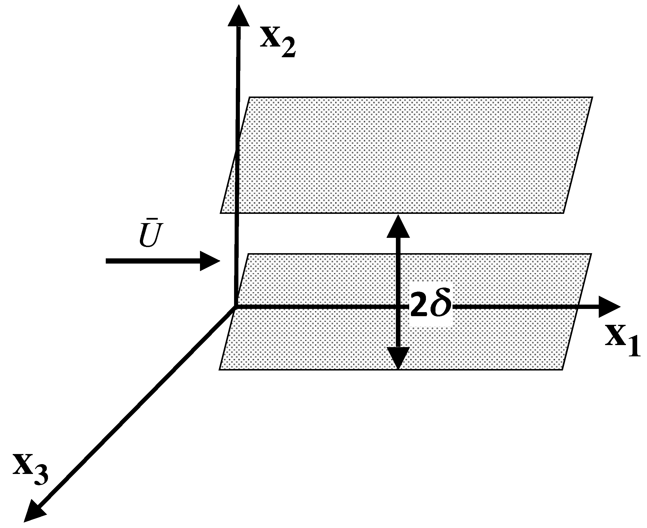
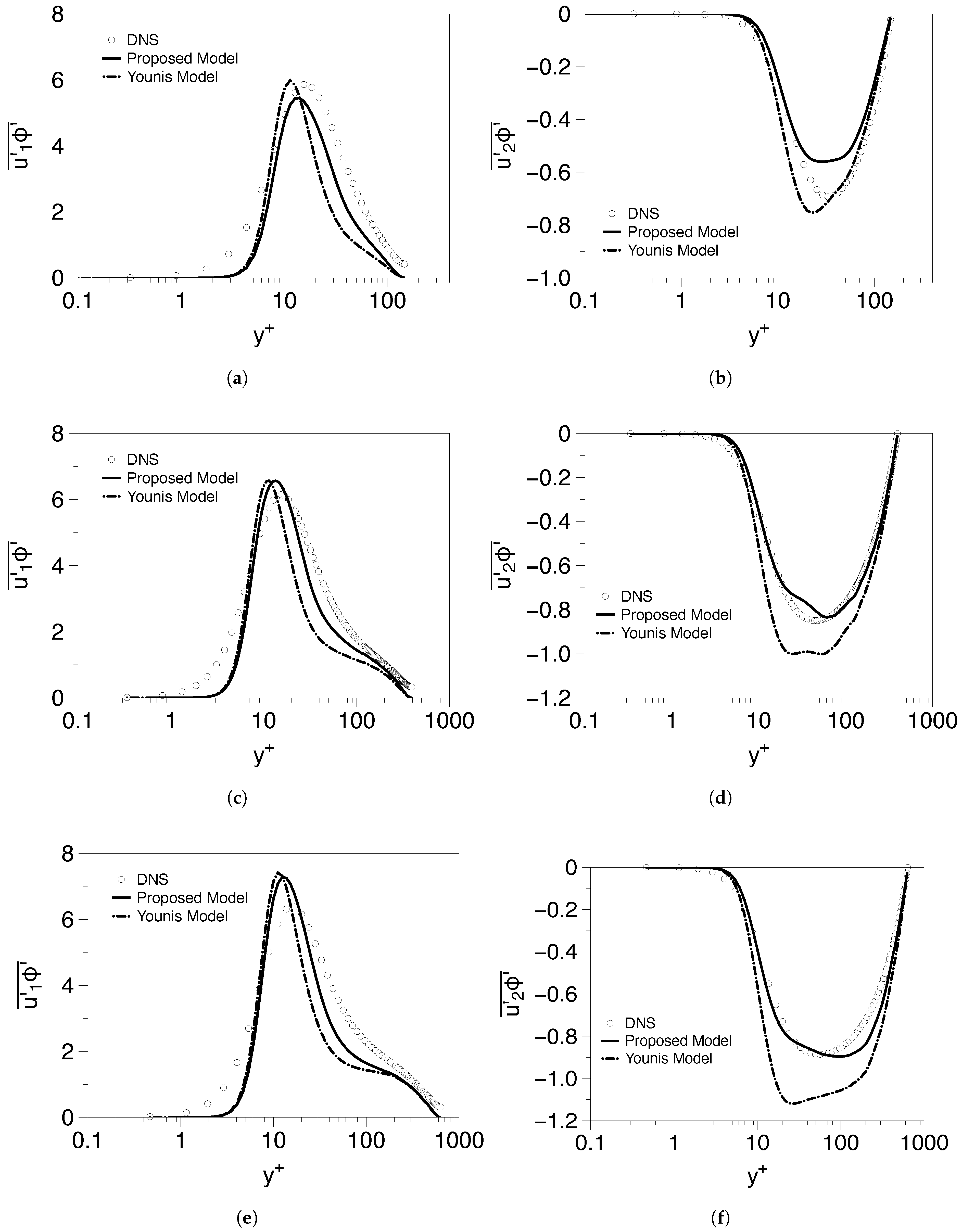
5.1. Poiseuille Flows

We evaluate model performance at fully-developed turbulent channel flows for a wide range of friction Reynolds numbers, particularly $R{e}_{\tau }=150,395,640,995,2013$ and 4088. For all cases, non-slip boundary condition is adopted in the wall-normal direction (i.e., at the top and bottom walls) while the scalar boundary condition is uniform scalar-flux on both walls.

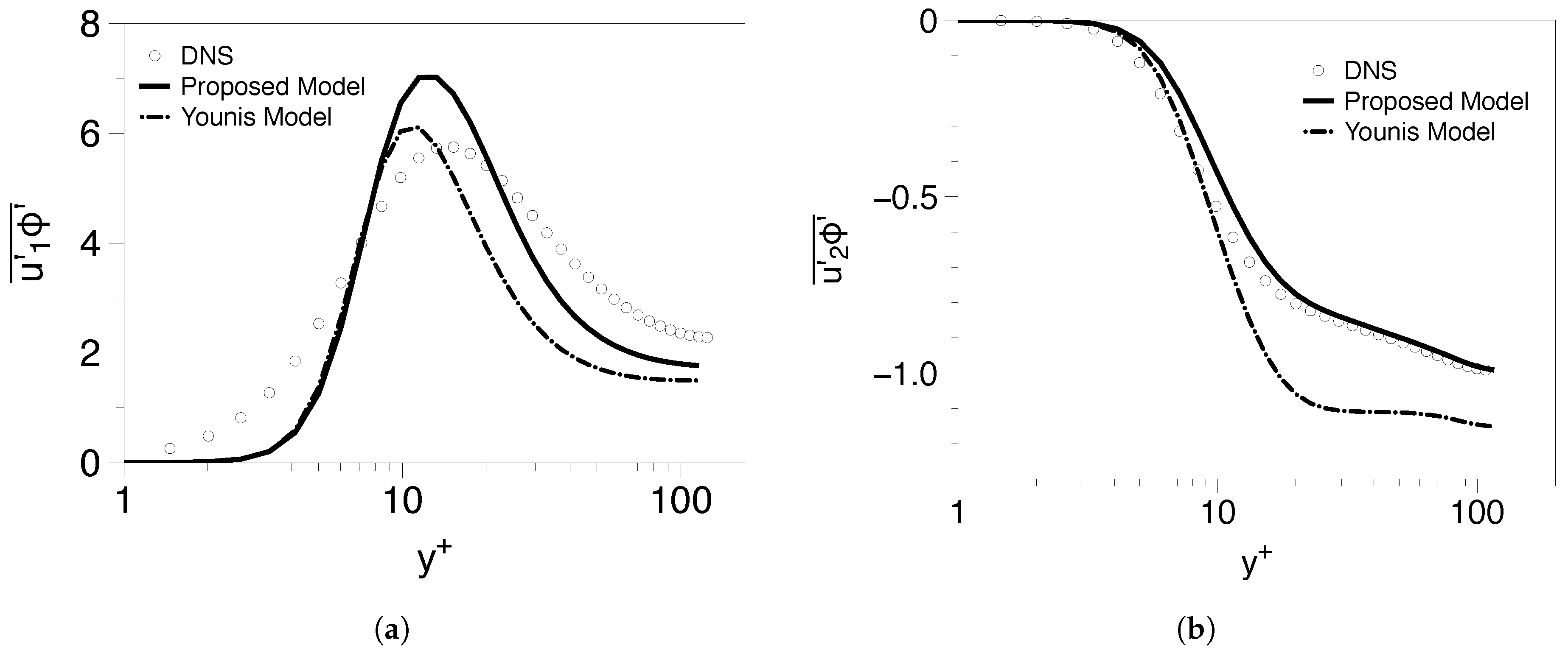
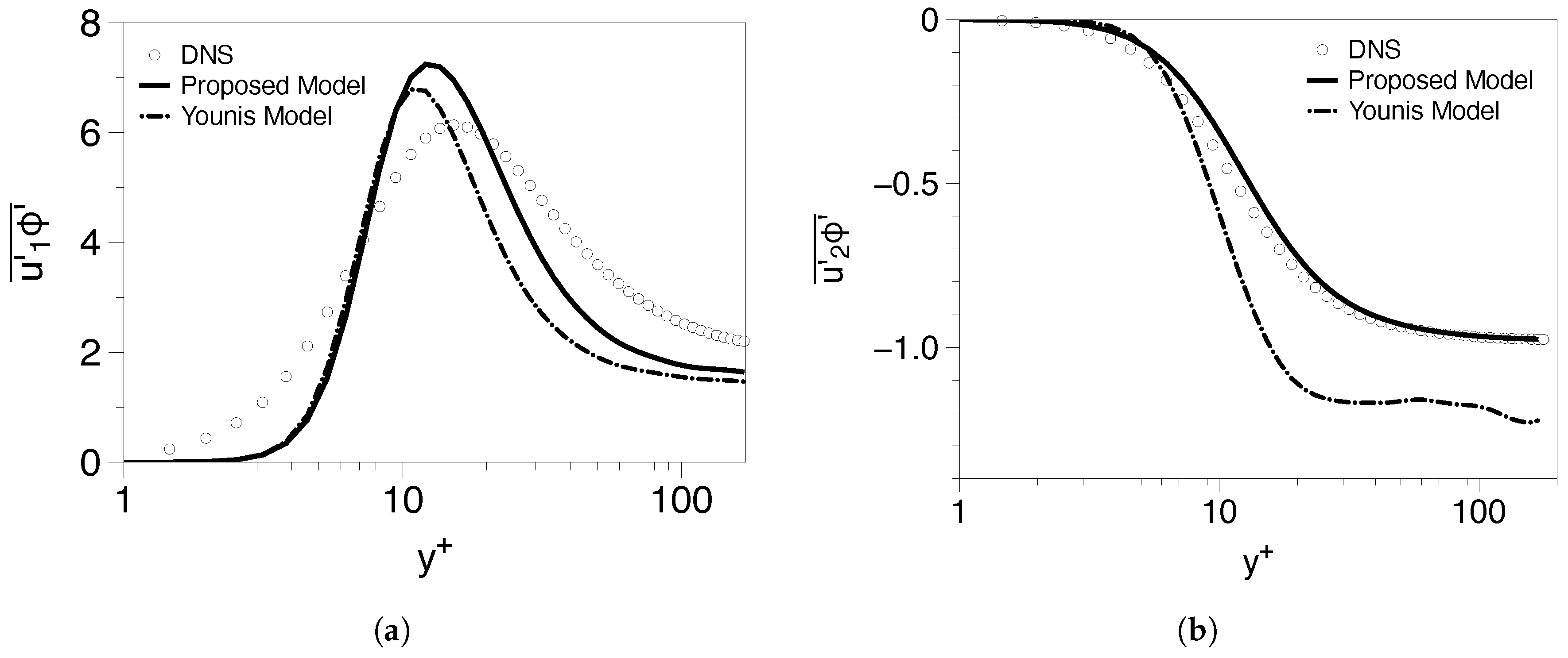
5.1.1. Low Reynolds Number Cases

We initially consider three different low Reynolds number cases, namely, $R{e}_{\tau }=150,395$, and 640. The quality of the predictions is compared with the corresponding DNS results [29,34,35]. Figure 3 compares the turbulent scalar-fluxes as obtained from the present model and the Younis model for the three cases. Solid line denotes the proposed model and dash-dotted line denotes Younis’ model. Symbols denote the DNS results. For all cases, both models provide reasonable agreement with DNS regarding the near-wall peak value of the streamwise component. In addition, both closures underestimate the value of this component further away from the wall, while the predictions of the proposed closure are closer to the DNS results. Contrary to algebraic closures, DNS predict non-zero values for the streamwise component at the channel centerline. This happens because the turbulent scalar field is being transported by the mean flow or the turbulence. These transport processes constitute a non-local mechanism that cannot be captured by a rational algebraic closure [15]. Except from the lowest $R{e}_{\tau }$ case, the proposed model achieves a considerably better agreement than Younis’ model regarding the normal flux at the entire region. In particular, the current model accurately captures the near-wall behavior of the fluxes, while it exhibits a mild overestimation of the magnitude beyond $y^{+}\approx 80$ for $R{e}_{\tau }=640$, still being able to produce satisfactory results.

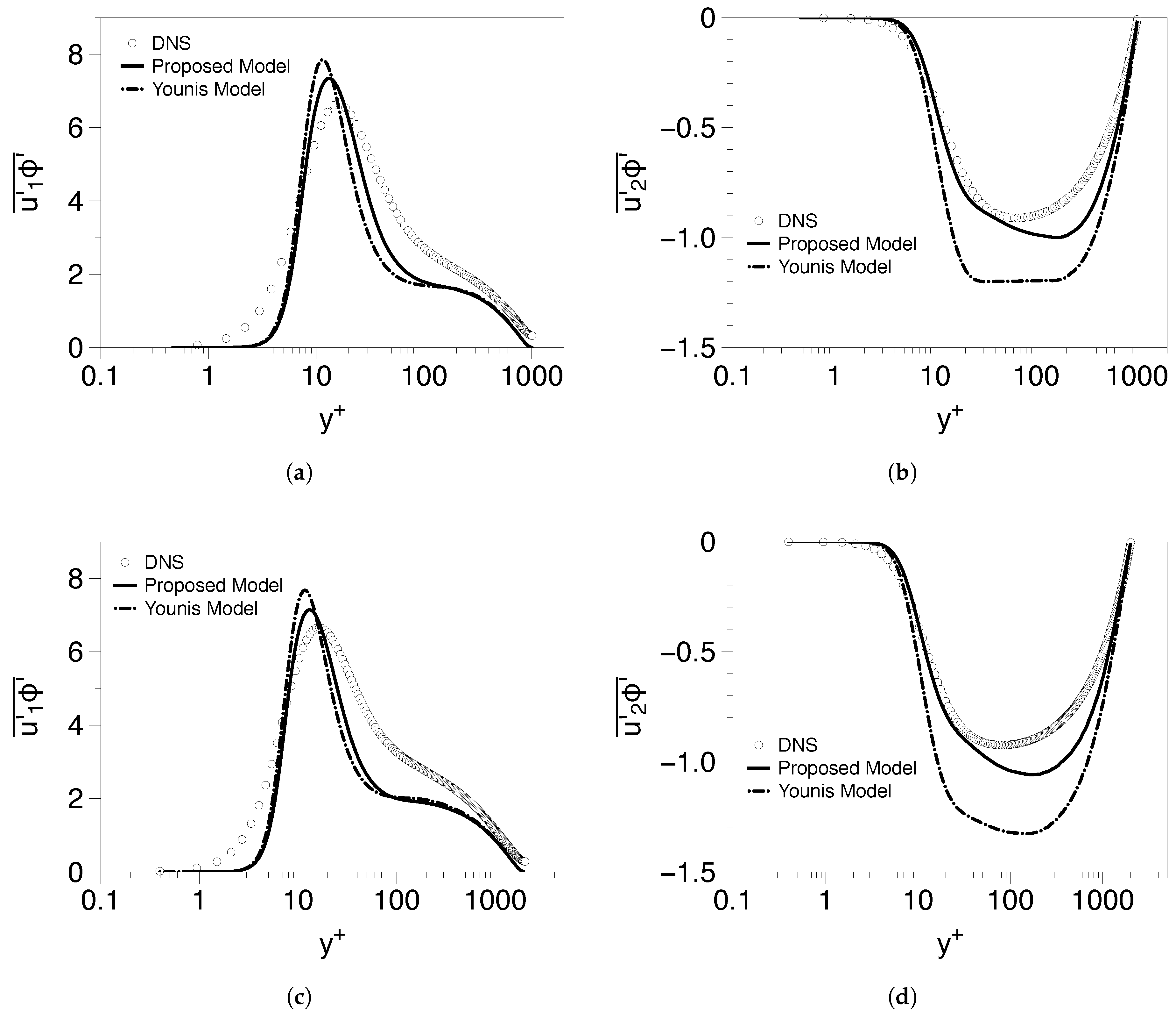
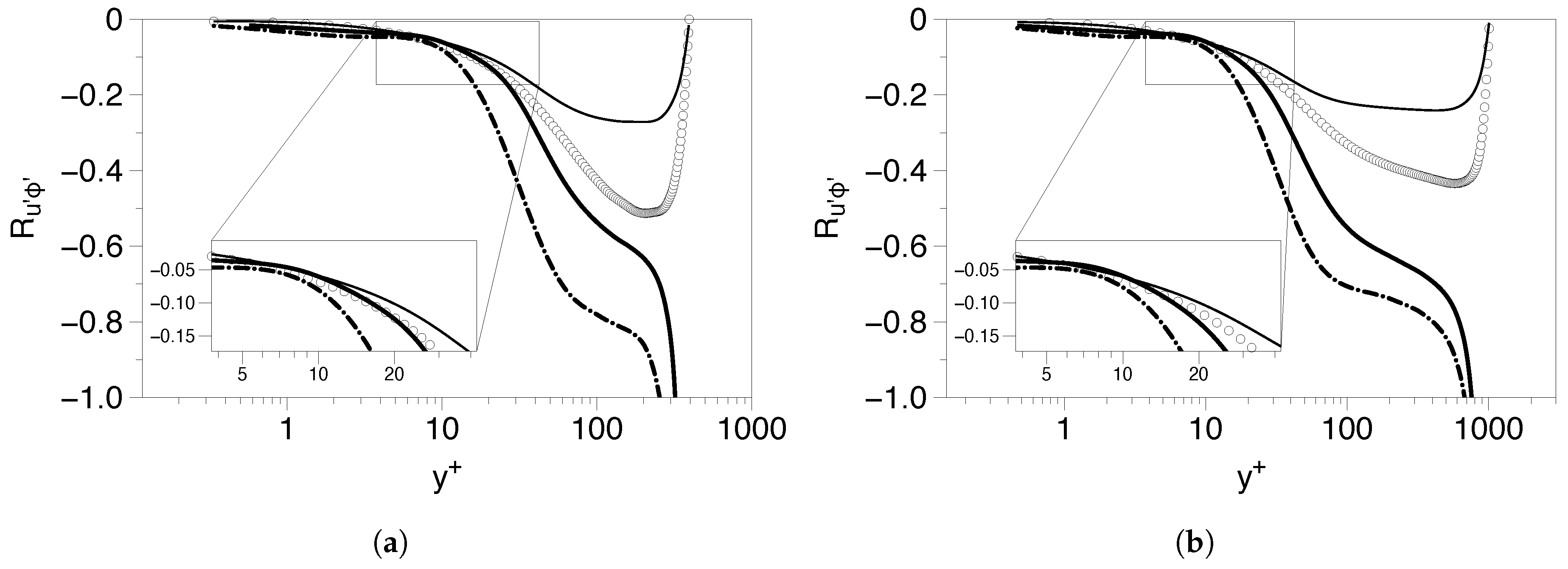
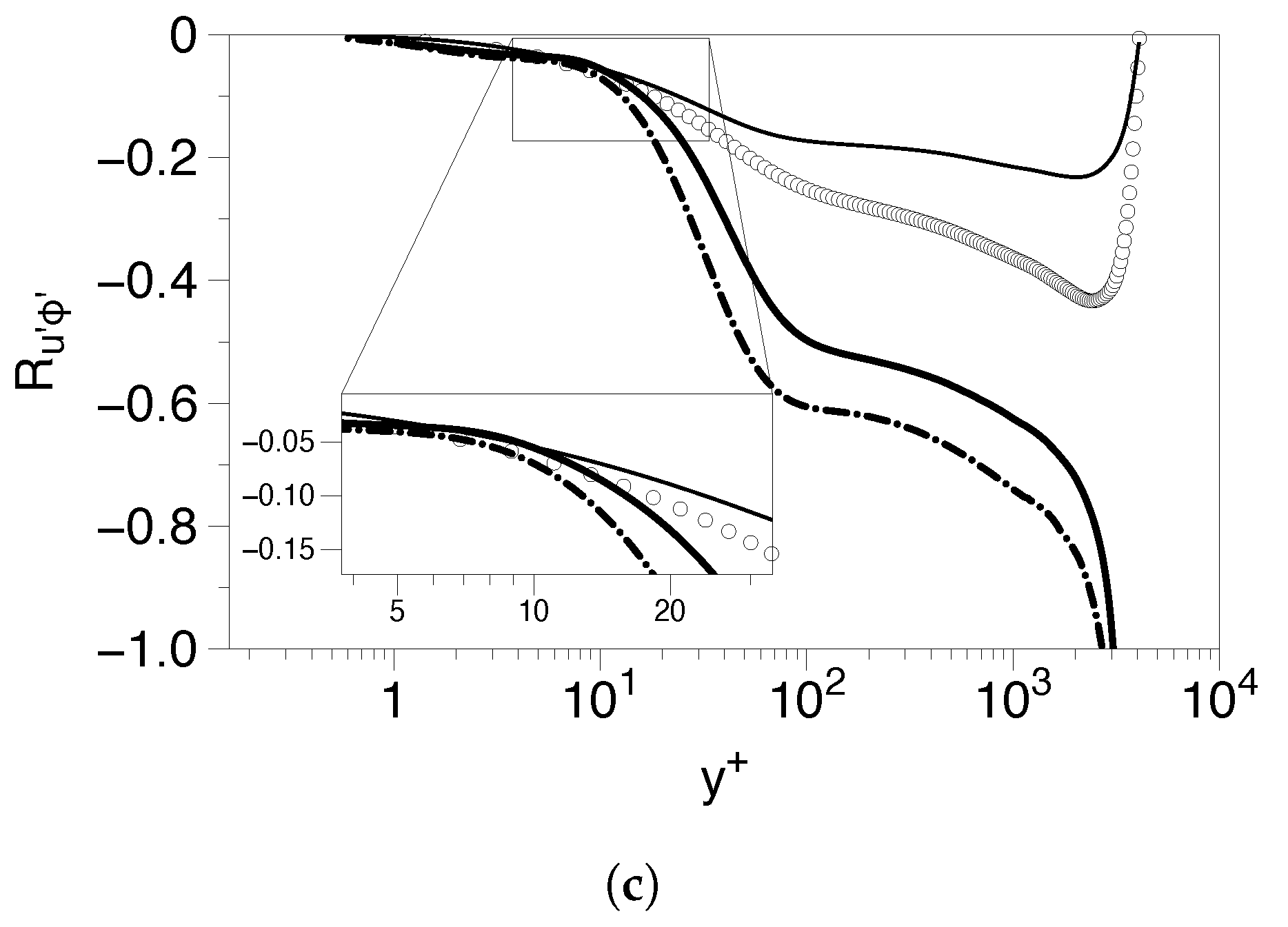
5.1.2. High Reynolds Number Cases

Next (Figure 4), we investigate model performance at higher Reynolds numbers than before, particularly $R{e}_{\tau }=995,2013$ and 4088, against available DNS results [36,37].

Regarding the streamwise flux component, the current model captures well the near-wall peak magnitude for all cases, being able to properly adjust to the presence of high-shear rates. Furthermore, it achieves very good agreement with the DNS predictions for the normal component at the near-wall region ($y^{+}<40$) for all cases, suggesting that the use of the terms involving Reynolds stress is enough to properly capture the highly anisotropic correlations between $u_2^{\prime }$ and ${\varphi }^{\prime }$ that exist at the near-wall region. As in the $R{e}_{\tau }=640$ case, we observe its tendency to overestimate, although much milder than Younis’ model, the magnitude of the normal flux beyond the slope change.

5.1.3. Inclination Angle of the Scalar-Flux Vector Near the Wall Boundary

Here, we further investigate the near-wall performance of the proposed closure. A useful parameter for that purpose is the scalar-flux ratio $R_{u^{\prime }{\varphi }^{\prime }}$, defined in Equation (13). Figure 5 shows a comparison of the scalar-flux ratio predictions of both models with the corresponding DNS data at three different Reynolds number cases, namely, $R{e}_{\tau }=395,995$ and 4088. For comparison purposes, we have also included the DNS predictions for $R_{12}/R_{11}$ as this ratio is expected to vary as scalar-flux ratio in the near-wall region, as already mentioned in Section 3. We observe that the proposed model achieves better agreement with the DNS results for all cases. Especially for $R{e}_{\tau }=395$, it captures accurately the near-wall limit up to $y^{+}\approx 30$, in accordance with the previous discussion. This is attributed to the dominant role that $C_5$-related term plays in the buffer layer for both flux-components, as already shown in Figure 1, which exhibits the proper near-wall physical behavior (see discussion in Section 3). In contrast, Younis’ model fails to capture this limiting behavior for $y^{+}>10$, partly because no term appearing in its model Equation (6) captures the correct inclination of the flux vector.

5.2. Couette Flows

We now ascertain the performance of the models in a fully-developed Couette flow with the top wall moving at constant speed $u_w$ relative to the bottom wall. As a result, the mean flow is driven by the shear stress due to the relative movement between top and bottom walls, while the scalar difference between the top and bottom walls is kept constant. We consider two cases at relatively low Reynolds numbers, particularly $R{e}_w=\frac{2u_w\delta }{\nu }=8600$ and 12,800, for which detailed DNS data are provided in [28]. Figure 6 and Figure 7 show a comparison between the two models for the scalar-flux components with the corresponding DNS results. Compared to Younis closure, the proposed model tends to overestimate the near-wall peak value of the streamwise component, while it provides better estimations beyond $y^{+}>20$. Regarding the normal component, predictions agree quite well with the DNS data for both cases, especially for the higher $R{e}_w$-case, while Younis’ model underestimates the wall-normal component outside the viscous sublayer ($y^{+}>10$).

5.3. Higher Pr Case

As mentioned in Section 3, Kim and Moin [24] studied the near-wall behavior of the scalar-flux vector in turbulent channel flows for a wide range of Prandtl numbers. As a result, they observed mild changes in scalar ratio $R_{u^{\prime }{\varphi }^{\prime }}$ with increasing Prandtl number in the range of $Pr\ge 0.71$. The above observation, along with the fact that the proposed model does not explicitly depend on this parameter, has motivated us to evaluate model performance at higher $Pr$ than 0.7. In particular, we consider a Poiseulle flow at $R{e}_{\tau }=395$ and $Pr=7$, for which detailed DNS data are provided by Kawamura [28]. Boundary conditions are identical to the ones described in Section 5.1. Comparison is made again with Younis’ model, which directly depends on $Pr$ through damping function $f_{C1}$ as indicated in Equation (10). Figure 8 shows a comparison between both models with the corresponding DNS results for the scalar-flux components. Compared to Younis’ model, the proposed model tends to underpredict the near-wall peak value of the streamwise component, whereas it provides better predictions for $y^{+}>15$. As in all previous cases, both models exhibit a sharp reduction of the profile while moving away from the walls. Regarding the normal component, the present model achieves a much better agreement with the DNS results outside the viscous sublayer ($y^{+}>10$).

Figure 9 shows the corresponding predictions for the scalar ratio $R_{u^{\prime }{\varphi }^{\prime }}$. The proposed model agrees reasonably well with the DNS results for $y^{+}<15$. Compared to Younis’ model, the proposed model provides much better predictions for this ratio in the entire domain.

6. Summary and Conclusions

In this study, we have proposed an explicit algebraic closure for the turbulent scalar-flux vector based on the general formulation of Younis, which is essentially an extended version of the model proposed by Abe and Suga (14) through the inclusion of an extra term involving products between the gradients of the mean velocity and scalar field. This closure consists of three terms, making it simpler than Younis’ model and an elegant choice for use in general-purpose computational codes. It is also motivated by the “effective gradients" hypothesis, which postulates that turbulence–turbulence interactions provide a gradient that acts supplementary to the mean shear, thus giving an alternative physical interpretation of the proposal compared to other closures. To minimize model bias to inhomogeneous applications, the values of the model coefficients are determined based on existing LES predictions of homogeneous shear flows in the presence of arbitrary mean scalar gradients, while a simple correction function was applied to the $C_3$-term to properly capture the near-wall behavior. In order to test the quality of the proposed model, we have considered different types of channel flows, particularly Poiseuille and Couette flows, for a broad range of Reynolds numbers and $Pr=0.7$. The proposed model performs satisfactorily in Couette flows at two different Reynolds numbers, especially for the normal component, thus showing its sensitivity to the near-wall inclination of the scalar-flux field. Regarding Poiseuille flows, fair predictions are obtained for both flux components, with the model being able to well capture the near-wall peak magnitude of the streamwise component regardless the Reynolds number choice. Furthermore, the proposed model accurately captures the near-wall behavior for the scalar ratio $R_{u^{\prime }{\varphi }^{\prime }}$ for distances up to $y^{+}\approx 30$ ($R{e}_{\tau }=395$), significantly further than Younis’ model ($y^{+}\approx 10$). Model performance is further evaluated in a Poiseuille flow at a higher Prandtl number ($Pr=7$) that typically occurs in marine applications and water–boundary interaction, again providing reasonable predictions. The above cases served as a guidance regarding the role of the different terms appearing in the algebraic expressions, showing the ability of the proposal to capture the levels of misalignment between the different flux components. As part of future work, we intend to propose an extension of the proposed RANS-based model so that it properly accounts for Prandtl effects under different scenarios. Special attention will be given to $Pr$ numbers that typically occur in aerated flows. To achieve that, we intend to consider several cases that involve Prandtl numbers in the range of 1 to 10, and perform computations to examine the sensitivity of the closure to the predicted stress fields. Furthermore, relevant experimental studies will be performed in the future to provide data for a comparative study between different turbulence models for the case of water flow around a monopile.

References

1. Smagorinsky, J. General circulation experiments with the primitive equations: I. The basic experiment. Mon. Weather Rev. 1963, 91, 99–164. [Google Scholar] [CrossRef]
2. Verstappen, R. When does eddy viscosity damp subfilter scales sufficiently? J. Sci. Comput. 2011, 49, 94–110. [Google Scholar] [CrossRef] [Green Version]
3. Rozema, W.; Bae, H.J.; Moin, P.; Verstappen, R. Minimum-dissipation models for large-eddy simulation. Phys. Fluids 2015, 27, 085107. [Google Scholar] [CrossRef] [Green Version]
4. Nicoud, F.; Ducros, F. Subgrid-scale stress modelling based on the square of the velocity Gradient Tensor. Flow Turbul. Combust. 1999, 62, 183–200. [Google Scholar] [CrossRef]
5. Verstappen, R. How much eddy dissipation is needed to counterbalance the nonlinear production of small, unresolved scales in a large-eddy simulation of turbulence? Comput. Fluids 2016, 176, 276–284. [Google Scholar] [CrossRef]
6. Trias, F.; Folch, D.; Gorobets, A.; Oliva, A. Building proper invariants for eddy-viscosity subgrid-scale models. Phys. Fluids 2015, 27, 065103. [Google Scholar] [CrossRef] [Green Version]
7. Rozema, W.; Verstappen, R.W.C.P.; Veldman, A.E.P.; Kok, J.C. Low-Dissipation Simulation Methods and Models for Turbulent Subsonic Flow. Arch. Comput. Methods Eng. 2018, 27, 299–330. [Google Scholar] [CrossRef] [Green Version]
8. Batchelor, G. Diffusion in a field of homogeneous turbulence. Aust. J. Sci. Res. Ser. A 1949, 2, 437–450. [Google Scholar] [CrossRef]
9. Daly, B.; Harlow, F. Transport equations of turbulence. Phys. Fluids 1970, 13, 2634–2649. [Google Scholar] [CrossRef]
10. Suga, K.; Abe, K. Nonlinear eddy viscosity modelling for turbulence and heat transfer near wall and shear-free boundaries. Int. J. Heat Fluid Flow 2000, 21, 37–48. [Google Scholar] [CrossRef]
11. Rodi, W. The Prediction of Free Turbulent Boundary Layers by Use of a Two-Equation Model of Turbulence. Ph.D. Thesis, Department of Heat Transfer, Imperial College, London, UK, 1972. [Google Scholar]
12. Girimaji, S.; Balachandar, S. Analysis and modeling of buoyancy-generated turbulence using numerical data. Int. J. Heat Mass Trans. 1998, 41, 915–929. [Google Scholar] [CrossRef]
13. Wikstrom, P.; Wallin, S.; Johansson, A. Derivation and investigation of a new explicit algebraic model for the passive scalar flux. Phys. Fluids 2000, 12, 688–702. [Google Scholar] [CrossRef]
14. Lazeroms, W.; Brethouwer, G.; Wallin, S.; Johansson, A. An explicit algebraic Reynolds-stress and scalar-flux model for stably stratified flows. J. Fluid Mech. 2013, 723, 91–125. [Google Scholar] [CrossRef] [Green Version]
15. Younis, B.; Speziale, C.; Clark, T. A rational model for the turbulent scalar fluxes. Proc. R. Soc. A 2005, 461, 575–594. [Google Scholar] [CrossRef]
16. Younis, B.; Weigand, B.; Spring, S. An Explicit Algebraic Model for Turbulent Heat Transfer in Wall-Bounded Flow With Streamline Curvature. J. Heat Transf. 2007, 129, 425–433. [Google Scholar] [CrossRef]
17. Dakos, T.; Gibson, M. On modelling the pressure terms of the scalar flux equations. In Turbulent Shear Flows 5; Springer: Berlin/Heidelberg, Germany, 1987; pp. 7–18. [Google Scholar]
18. Yoshizawa, A. Statistical analysis of the anisotropy of scalar diffusion in turbulent shear flows. Phys. Fluids 1985, 28, 3226–3231. [Google Scholar] [CrossRef]
19. Kaltenbach, H.; Gerz, T.; Schumann, U. Large-eddy simulation of homogeneous turbulence and diffusion in stably stratified shear flow. J. Fluid Mech. 1994, 280, 1–40. [Google Scholar] [CrossRef] [Green Version]
20. Kim, J.; Moin, P.; Moser, R. Turbulence Statistics in Fully Developed Channel Flow at Low Reynolds Number. J. Fluid Mech. 1987, 177, 133–166. [Google Scholar] [CrossRef] [Green Version]
21. Younis, B.; Weigand, B.; Mohr, F.; Schmidt, M. Modeling the Effects of System Rotation on the Turbulent Scalar Fluxes. J. Heat Transf. 2010, 132, 051703. [Google Scholar] [CrossRef]
22. Launder, B. On the computation of convective heat transfer in complex turbulent flows. J. Heat Transf. 1988, 110, 1112–1128. [Google Scholar] [CrossRef]
23. Abe, K.; Suga, K. Towards the development of a Reynolds-averaged algebraic turbulent scalar-flux model. Int. J. Heat Fluid Flow 2001, 22, 19–29. [Google Scholar] [CrossRef]
24. Kim, J.; Moin, P. Transport of Passive Scalars in a Turbulent Channel Flow. In Turbulent Shear Flows; Andre, J.C., Cousteix, J., Durst, F., Launder, B., Schmidt, F., Whitelaw, J., Eds.; Springer: Berlin/Heidelberg, Germany, 1989; Volume 6. [Google Scholar]
25. Jones, W.; Musonge, P. Closure of the Reynolds stress and scalar flux equations. Phys. Fluids 1987, 31, 3589–3604. [Google Scholar] [CrossRef]
26. Monin, A. On the symmetry of turbulence in the surface layer of air. Izv. Atmos. Ocean. Phys. 1965, 1, 45–54. [Google Scholar]
27. Launder, B.E. On the effects of a gravitational field on the turbulent transport of heat and momentum. J. Fluid Mech. 1975, 67, 569–581. [Google Scholar] [CrossRef]
28. Kawamura, H.; Abe, H.; Shingai, K. DNS of turbulence and heat transport in a channel flow with different Reynolds and Prandtl numbers and boundary conditions. In Proceedings of the 3rd International Symposium on Turbulence, Heat and Mass Transfer, Nagoya, Japan, 3–6 April 2000; Nagano, Y., Hanjalic, K., Tsuji, T., Eds.; Aichi Shuppan: Tokyo, Japan, 2000; Volume 6. [Google Scholar]
29. Kozuka, M.; Seki, Y.; Kawamura, H. Direct Numerical Simulation Data Base for Turbulent Channel Flow with Heat Transfer. Available online: https://www.rs.tus.ac.jp/t2lab/db/ (accessed on 5 October 2020).
30. Kassinos, S.; Reynolds, W. A Structure-Based Model with Stropholysis Effects; Annual Research Briefs; Center for Turbulence Research, NASA Ames/Stanford University: Santa Clara County, CA, USA, 1998; pp. 197–209. [Google Scholar]
31. Panagiotou, C.; Kassinos, S. A structure-based model for the transport of passive scalars in homogeneous turbulent flows. Int. J. Heat Fluid Flow 2016, 57, 109–129. [Google Scholar] [CrossRef]
32. Panagiotou, C.; Kassinos, S. A structure-based model for transport in stably stratified homogeneous turbulent flows. Int. J. Heat Fluid Flow 2017, 65, 309–322. [Google Scholar] [CrossRef]
33. Panagiotou, C.; Stylianou, F.; Kassinos, S. Structure-based transient models for scalar dissipation rate in homogeneous turbulence. Int. J. Heat Fluid Flow 2020, 82, 108557. [Google Scholar] [CrossRef]
34. Tomita, Y.; Kasagi, N.; Kuroda, A. Establishment of the Direct Numerical Simulation Databases of Turbulent Transport Phenomena. Available online: https://thtlab.jp/ (accessed on 5 November 2020).
35. Abe, H.; Kawamura, H.; Matsuo, Y. Surface heat-flux fluctuations in a turbulent channel flow up to Reτ=1020 with Pr=0.025 and 0.71. Int. J. Heat Fluid Flow 2004, 25, 404–419. [Google Scholar] [CrossRef]
36. Pirozzoli, S.; Bernardini, M.; Orlandi, P. Passive scalars in turbulent channel flow at high Reynolds number. J. Fluid Mech. 2016, 788, 614–639. [Google Scholar] [CrossRef] [Green Version]
37. Pirozzoli, S.; Bernardini, M.; Orlandi, P. Turbulent Channel Flow With Passive Scalars—DNS Database Up to Reτ = 4000. Available online: http://newton.dma.uniroma1.it/scalars/stat/ (accessed on 5 November 2020).
Figure 1. Top: Predictions of the proposed model for the (a) streamwise and (b) normal scalar-flux components as a function of the distance from the wall y + . Symbols denote the DNS results of [29] for channel flow at R e τ = 395 and P r = 0.71 . Bottom: Balance between the individual terms appearing in the model Equation (15) for the (c) streamwise and (d) wall-normal scalar-flux components.
Jmse 08 00916 g001
Figure 2. Flow configuration and coordinate system.
Jmse 08 00916 g002
Figure 3. Model predictions for the scalar-flux components for a channel flow at R e τ = 150 (a,b), R e τ = 395 (c,d), and R e τ = 640 (e,f).
Jmse 08 00916 g003
Figure 4. Model predictions for the scalar-flux components for a channel flow: R e τ = 955 (a,b), R e τ = 2013 (c,d), and R e τ = 4088 (e,f).
Jmse 08 00916 g004aJmse 08 00916 g004b
Figure 5. Model predictions for the scalar ratio R u ϕ for a Poiseuille flow at (a) R e τ = 395 , (b) R e τ = 995 , and (c) R e τ = 4088 . Comparison is made with DNS predictions for the stress ratio R 12 / R 11 (thin lines) and the scalar ratio (symbols). The thick solid line denotes the proposed model and the dash-dotted line denotes Younis’ model. Zoomed view refers to the near-wall region.
Jmse 08 00916 g005aJmse 08 00916 g005b
Figure 6. Model predictions for the (a) streamwise and (b) normal scalar-flux components for a Couette flow at R e w = 8600 .
Jmse 08 00916 g006
Figure 7. As in Figure 6 but for R e w = 12,800.
Jmse 08 00916 g007
Figure 8. Model predictions for the (a) streamwise and (b) normal scalar-flux component for a Poiseuille flow at R e τ = 395 and P r = 7 .
Jmse 08 00916 g008
Figure 9. Model predictions for the scalar ratio R u ϕ for a Poiseuille flow at R e τ = 395 and P r = 7 . Comparison is made with DNS predictions for the stress ratio R 12 / R 11 (thin line) and the scalar ratio (symbols). The thick solid line denotes the proposed model and dash-dotted line denotes Younis’ model. Zoomed view refers to the near-wall region.
Jmse 08 00916 g009
Publisher’s Note: MDPI stays neutral with regard to jurisdictional claims in published maps and institutional affiliations.