Nonlinear Fourier Analysis: Rogue Waves in Numerical Modeling and Data Analysis

Abstract
:| Contents | |
| 1. Introduction to Nonlinear Fourier Analysis | 2 |
| 2. Overview of Linear and Nonlinear Fourier Analysis | 7 |
| 2.1. Discussion of the Classical “Linear Model” | |
| 2.2. Overview of Linear Fourier Analysis and Its Capabilities | |
| 2.3. Development of Nonlinear Fourier Analysis | |
| 2.4. Quasiperiodic Fourier Series for Solving Nonlinear Wave Equations, Numerical Modeling and Data Analysis | |
| 2.5. Extending Quasiperiodicity to Almost Periodicity | |
| 2.6. The Sub Grid Scale Problem | |
| 3. The Nonlinear Schrödinger Equation (NLS) in Two-Spatial Dimensions | 12 |
| 3.1. The 2+1 NLS Equation | |
| 3.2. The Modulational Dispersion Relation | |
| 3.3. Goals of This and Future Papers | |
| 4. The Nonlinear Spectrum of Two-Dimensional Wave Trains | 16 |
| 4.1. Plane Wave Solutions of the 2+1 NLS Equation | |
| 4.2. Modulation Dispersion Relation and Nonlinearity with Rotation | |
| 5. Constructing Asymptotic Solutions of the Two-Dimensional Schrödinger Equation | 22 |
| 5.1. NLS in 2+1 Dimensions | |
| 5.2. Computing the 2+1 NLS Equation Asymptotic Solutions Using Riemann Theta Functions | |
| 5.3. Generalize the 2+1 NLS Equation to Arbitrary Potential: The Hirota Method | |
| 5.4. Computation of the Nonlinear Spectrum in terms of the Riemann Matrix | |
| 5.5. Riemann Spectrum for the 1+1 NLS Equation | |
| 5.6. Riemann Spectrum for the 2+1 NLS Equation | |
| 6. The Physics of the NLFA Formulation | 28 |
| 6.1. Overview of the Formulation | |
| 6.2. A Simple Example for a Single Degree of Freedom | |
| 7. Numerical Methods of Nonlinear Fourier Analysis | 31 |
| 7.1. Overview of Numerical Methods for Determining the Nonlinear Spectrum in 2+1 Dimensions | |
| 7.2. Procedure for Computing the NLFA Spectrum of the Measured Surface Wave Elevation | |
| 7.3. Interpretation of Boxed Equation (106) | |
| 7.4. Quasiperiodic Fourier Structure of Measured Riemann Theta Functions | |
| 7.5. Numerical Analysis in Two Dimensions: Measurement of a Wave Field of the Sea Surface at | |
| 7.6. Numerical Analysis for a 1D Sea Surface Elevation | |
| 7.7. Concrete Example for a Single Degree of Freedom | |
| 7.8. Alternative General Notation | |
| 7.9. Primer on Nonlinear Fourier Analysis as a Theory of Nonlinearly Interacting Stokes Waves | |
| 7.10. Modelling the Surface Wave Elevation | |
| 7.11. Computing the Frequencies for Time Series Analysis and Modelling | |
| 7.11.1. The Linear Model | |
| 7.11.2. Linear Schrödinger Equation in 1+1 Dimensions | |
| 7.11.3. The Modulational Instability for 1+1 NLS | |
| 7.11.4. LSE in 2+1 Dimensions | |
| 7.11.5. The Modulational Instability in 2D | |
| 8. Application to Analysis of SINTEF Wave Tank Data | 57 |
| 9. Application to Analysis of Wave Data in Currituck Sound | 62 |
| 10. Application to Radar Data Assimilation and Modelling, and Real Time Prediction of Ocean Waves | 64 |
| 11. Summary and Discussion | 66 |
| Appendix A—What Is Fourier or Harmonic Analysis? | 67 |
| References | 70 |
1. Introduction to Nonlinear Fourier Analysis
- (1)
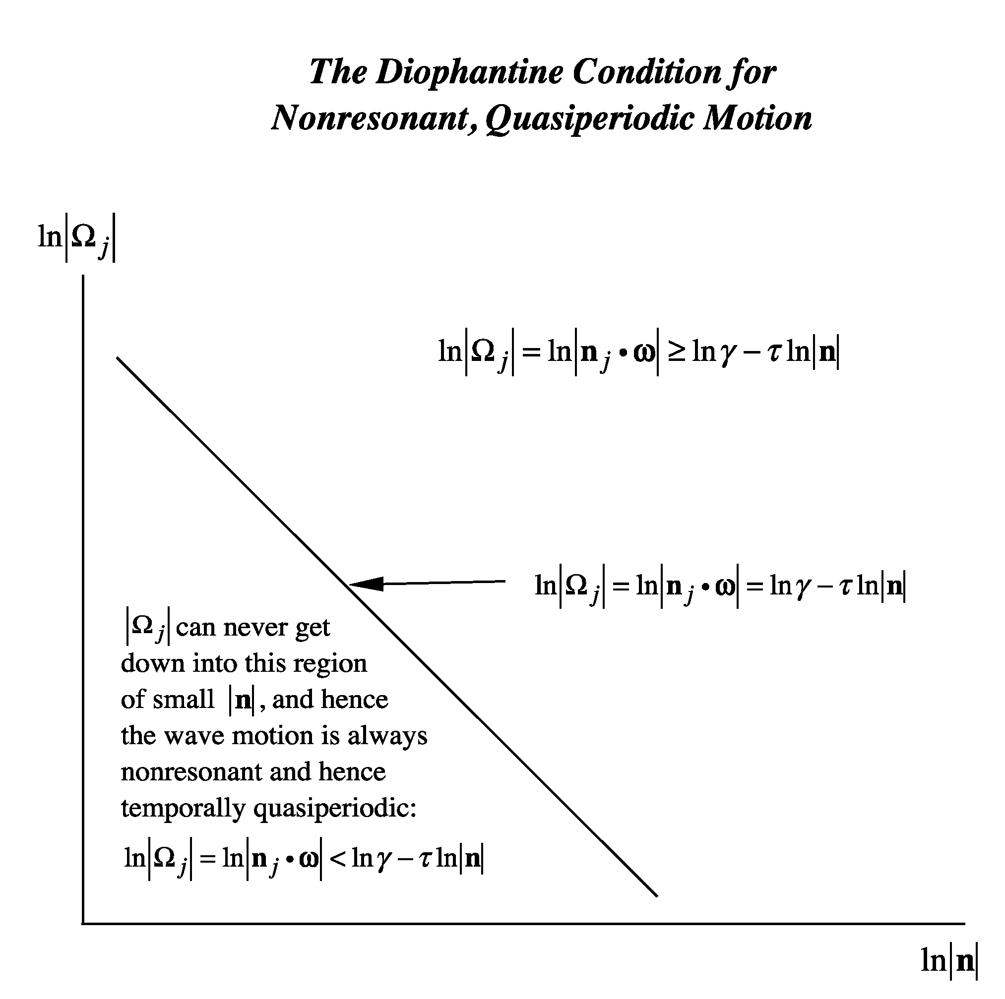
- Even though NLFA is itself a linear superposition of sine waves, the Fourier parameters are not the traditional ones of standard periodic Fourier analysis. NLFA leverages quasiperiodic Fourier series to describe nonlinear waves and the QPF parameters are particular, vast in number and are obtained with the mathematics of harmonic analysis (Bohl [22], Bohr [23], Besicovitch [24], Bochner [25,26] and Jessen [27]).
- (2)
- NLFA is applied to particular nonlinear wave equations whose exact spectral solutions are found using the inverse scattering transform (as this method is known in the United States, see [1]) or finite gap theory (as it is known in Russia, see Belokolos et al. [28]). Equations solvable by these methods are the well-known “soliton equations” such as the Korteweg-deVries (KdV), the Kadomtsev-Petviashvili (KP) and the nonlinear Schrödinger (NLS) equations. Equations of this type have “coherent structure” solutions such as Stokes waves, solitons, vortices, and breather trains. Integrable equations of this type are also known as “soliton theories.” The linear superposition law in item (1) above arises from soliton theories when periodic or quasiperiodic boundary conditions hold (see Osborne [1,2,3,4]).
- (3)
- The NLFA spectrum is a (Riemann) matrix, not a vector as in standard Fourier series. The diagonal elements of the Riemann matrix correspond to Stokes waves and the off-diagonal elements correspond to pair-wise interactions amongst the Stokes waves. NLFA is therefore a theory of Fourier analysis with Stokes wave basis functions. This contrasts to standard Fourier analysis, which is a theory of non-interacting sine wave basis functions. The dynamics of a nonlinear random wave train with many Stokes waves in the spectrum can be described only by quasiperiodic Fourier series, not by standard periodic Fourier series.
- (4)
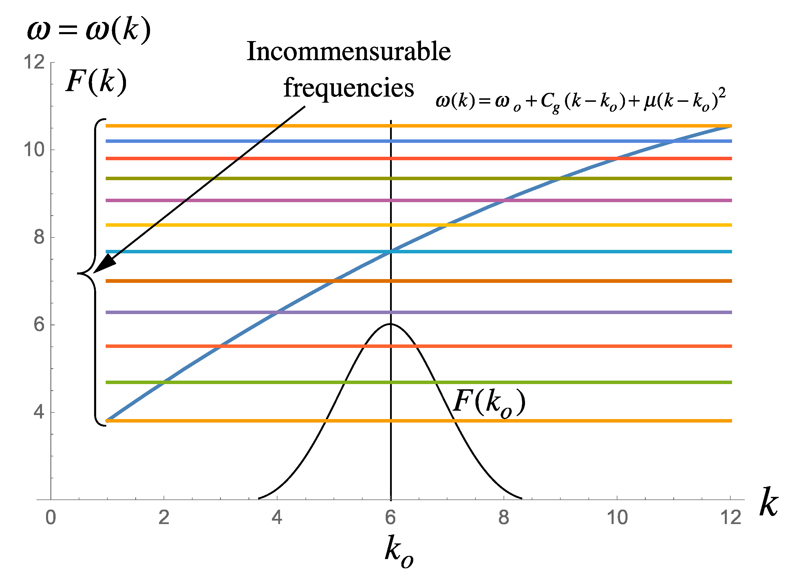
- The nonlinearity parameter of NLFA, called the Benjamin–Feir (BF) instability parameter , is proportional to the wave steepness divided by the spectral bandwidth (Osborne [1]):where is the carrier amplitude, is the carrier wave number and is the modulational wavenumber. Large steepness and small bandwidth give larger BF parameter and therefore greater nonlinearity, leading to breather trains.
- (5)
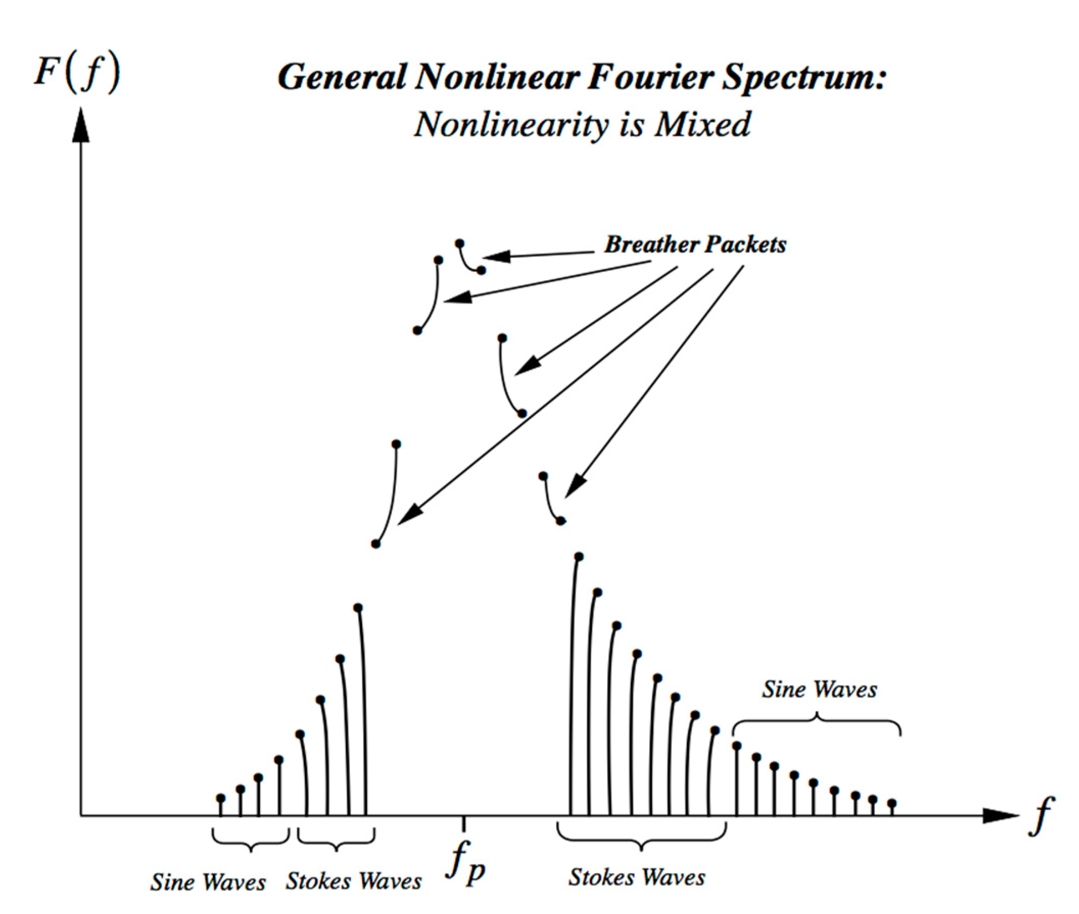
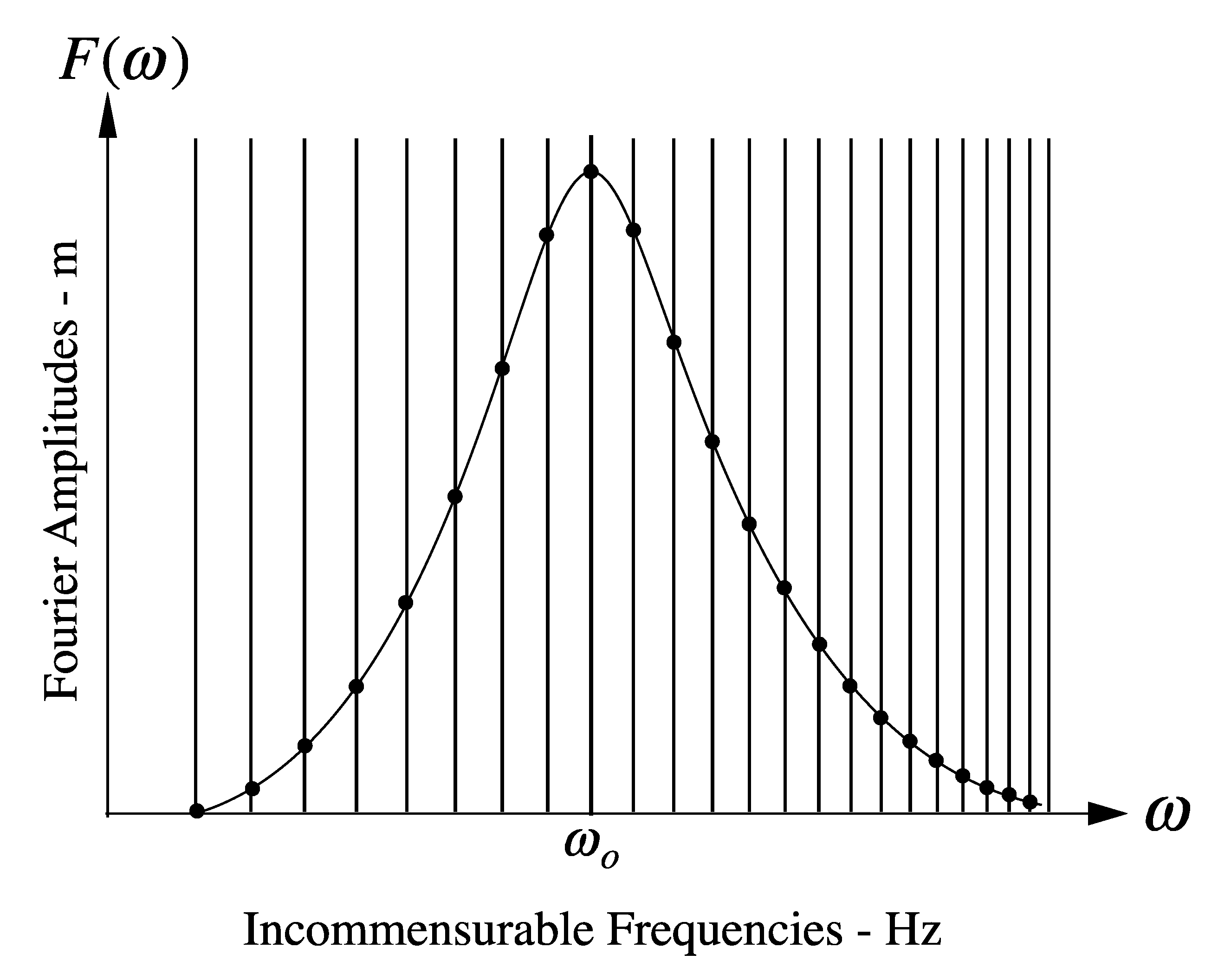
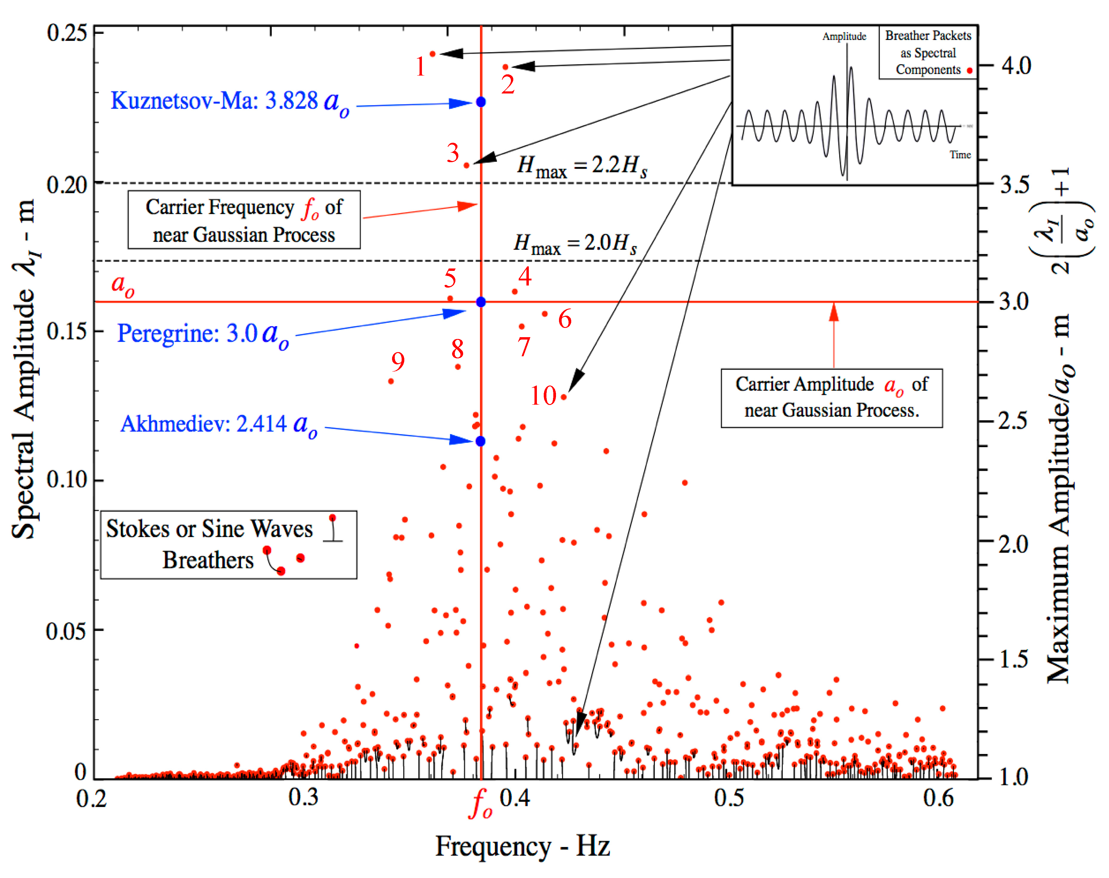
- When the BF parameter is much smaller than 1, the NLFA components are sine waves. When the BF parameter is larger, but still less than 1, the components are sine waves and Stokes waves. When the BF parameter exceeds 1, two Stokes waves in the spectrum phase lock together to form a type of nonlinear beat, most often called a breather wave train. Further increase of the BF parameter can lead to nonlinear spectra dominated by breather trains, often referred to as a rogue sea. There are also superbreather solutions, which consist of an infinite hierarchy of phase locked Stokes waves and breathers of increasing complexity. Breathers have been seen often in ocean waves, but up to now superbreathers have not been observed. Figure 1 gives a simple perspective of the typical ocean wave spectrum found by NLFA when all three types of Fourier modes are active in a particular energetic sea state.
- (6)
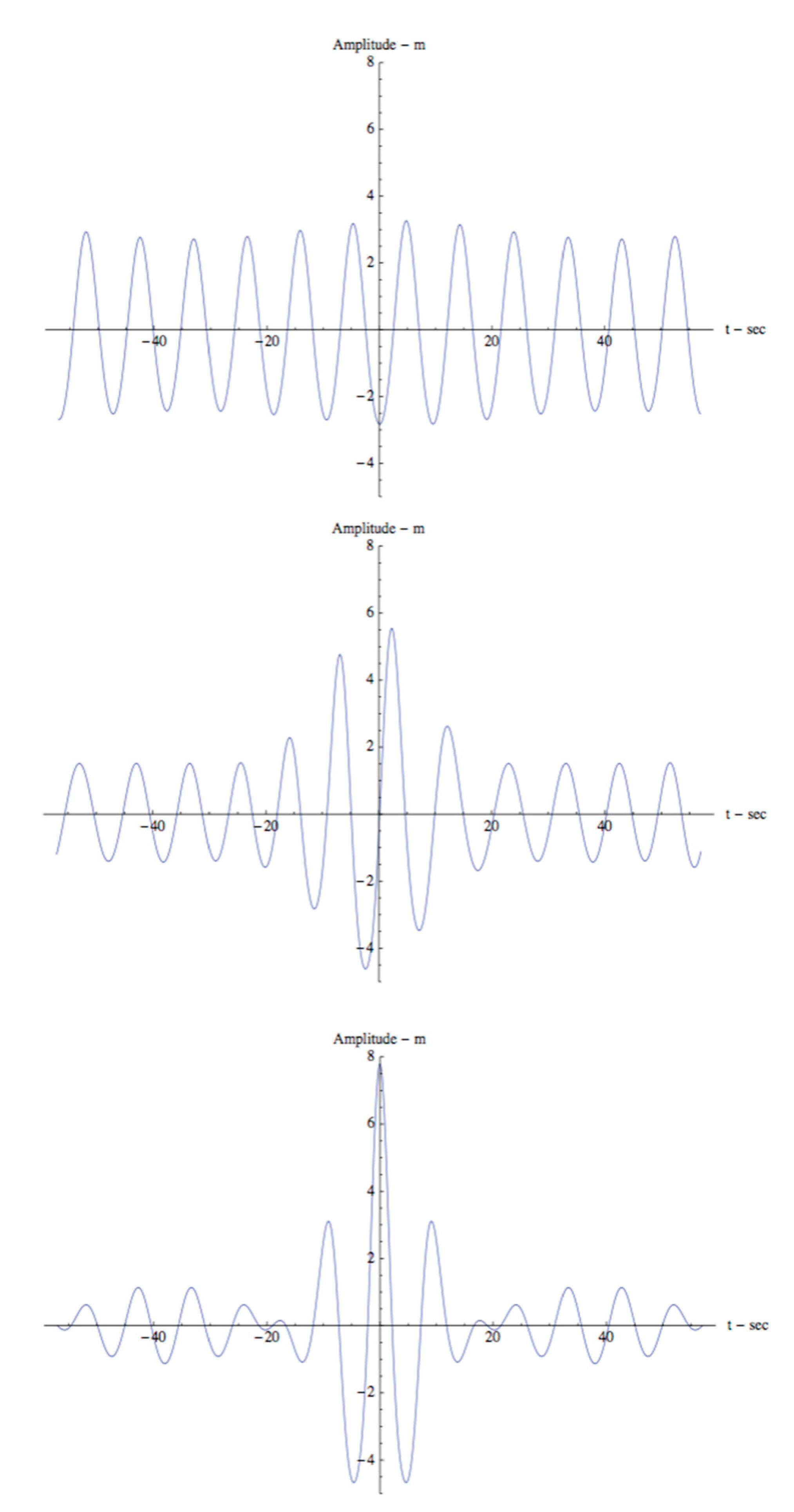
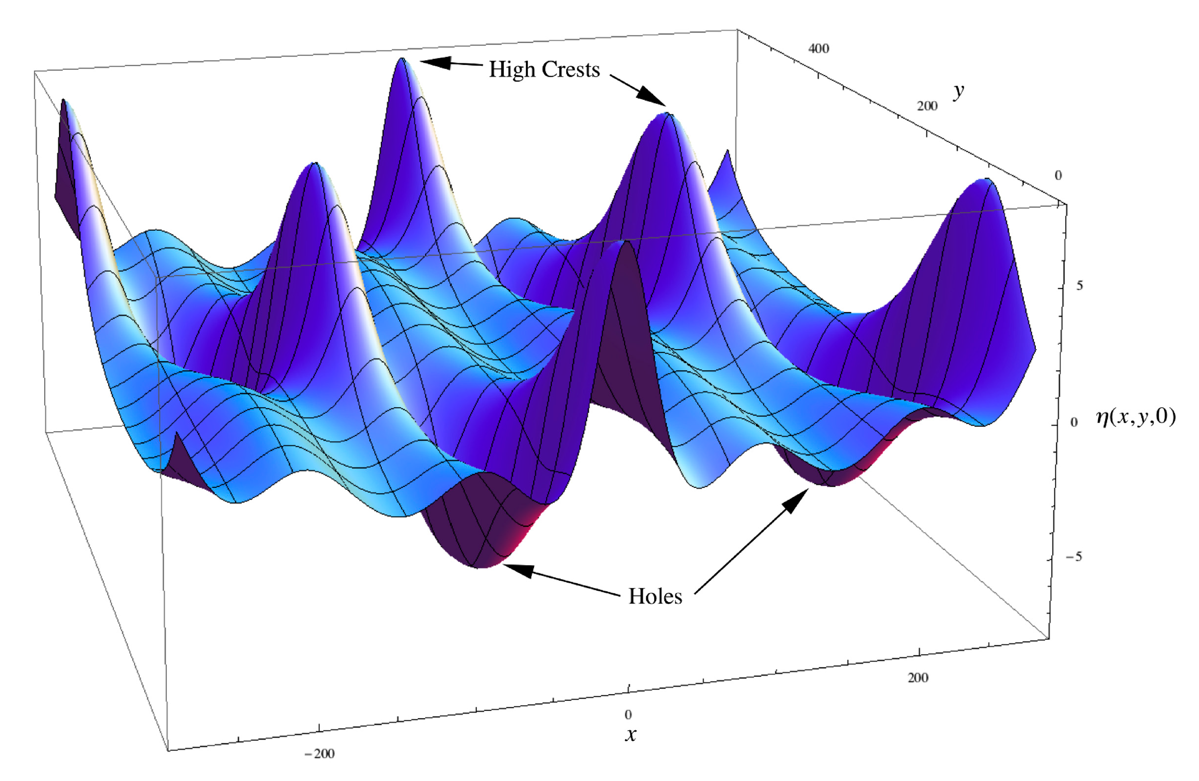
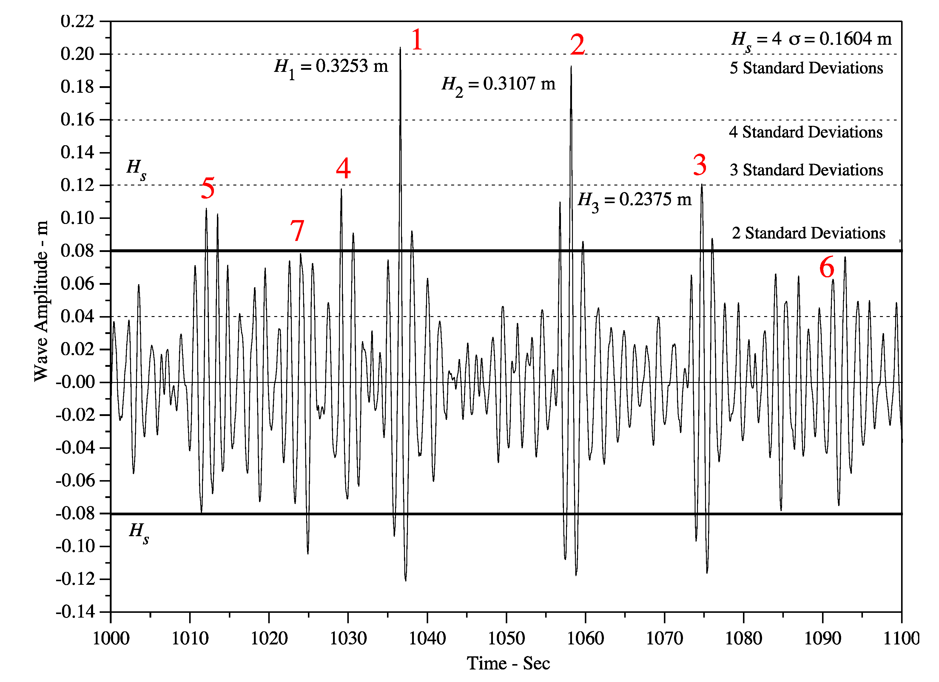
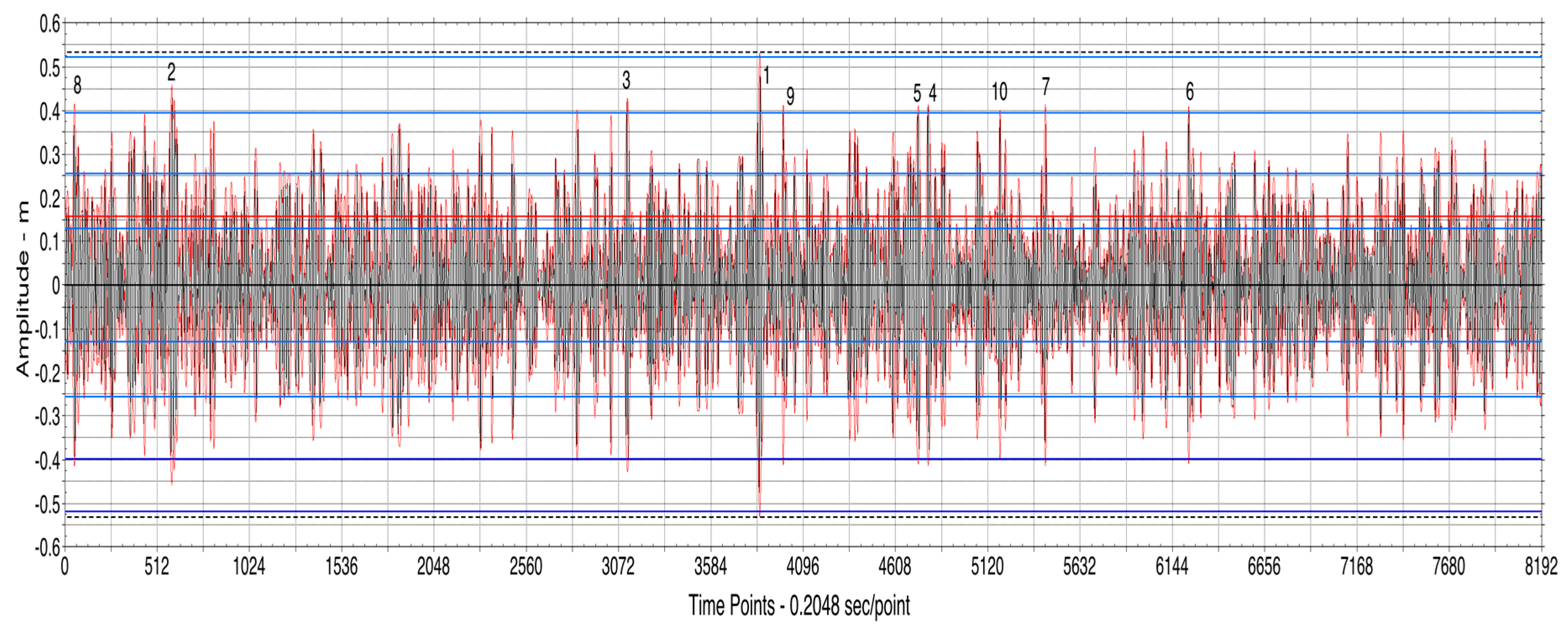
- Breathers have a coherent nonlinear dynamical behavior as they do not undergo linear dispersion as occurs in a linear packet, but instead maintain their packet shape during their evolution while their amplitudes oscillate up and down (they “breathe”), i.e., they are coherent structures. Breathers are a well-known source of rogue or freak waves in oceanic sea states [1,5]. Breather packets are single nonlinear Fourier modes in the NLFA spectrum of ocean waves and are “coherent structures” that mathematically correspond to “hyperbolic vortices” in the coherent turbulence of ocean waves (Osborne et al. [5]), just as “elliptic vortices” appear in classical 2D fluid turbulence. A breather can rise up to as much as three or four times the height of the background waves. The evolution of typical breather is shown in Figure 2.
- (1)
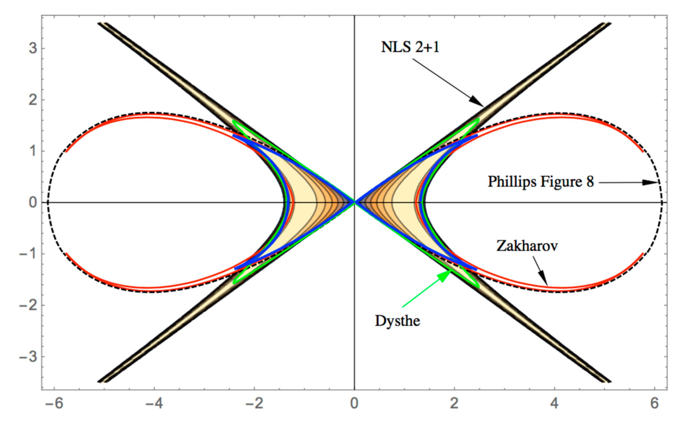
- NLFA as quasiperiodic Fourier series solve the well-known integrable nonlinear wave equations and approximately solve many others (Belokolos et al. [28], Eliasson et al. [29], Osborne [1], Osborne et al. [5]). This allows a direct approach for describing solutions of the KdV, KP, and nonlinear Schrödinger equations. Furthermore, at higher order, the Dysthe [30], Trulsen-Dysthe [31], and Zakharov [32,33] equations can be addressed using these series. At higher order still, the Zakharov equation can be studied with such series. Certain aspects of higher order modulation theory have been addressed by Kimmoun et al. [34].
- (2)
- (3)
- NLFA can be used for the computation of the directional spectra of measured space/time series and wave fields. This means that sine waves, Stokes waves, and breathers can have a range of directions in the directional spectrum.
- (4)
- NLFA can be used to develop nonlinear numerical models of wave fields [1]. These are the first class of numerical models that naturally maintain the coherent structures of nonlinear waves (Stokes waves and breathers) in the formulation. The numerical methods compute these coherent structures, which are nonlinear Fourier modes, as a matter of course in the numerical model.
- (5)
- Since NLFA is a linear superposition of sine waves, one can introduce a nonlinear random phase approximation by using random phases in the quasiperiodic Fourier series (Osborne [2,3,4] and Osborne et al. [5]). NLFA is different than the traditional random phase approximation because phase locking allows the formation of Stokes waves and breathers in the nonlinear spectrum. In this way, the nonlinear Fourier series are then viewed as nonlinear random processes. One can then compute correlation functions, power spectra, triple correlations, coherence functions, transfer functions, and many other properties of these stochastic processes analytically, even though they are fundamentally nonlinear (Osborne [1,2,3,4,5]).
- (6)
- One can analytically compute particle velocity kinematics under wave fields using quasiperiodic Fourier series. This leads to the idea that nonlinear transfer functions can be computed from quasiperiodic Fourier series, thus connecting wave amplitudes and particle velocity components.
- (7)
- Wave forces based upon Morison’s equation and diffraction theory can be computed analytically using NLFA. This allows nonlinear Fourier computations of wave forces on offshore structures, ships, breakwaters, etc. with NLFA.
- (8)
- Wind/Wave modeling can be improved with NLFA. This allows the specific implementation of rogue waves into forecasting/hindcasting models. Up to now, rogue waves have not been reliably predicted in forecasting models.
- (9)
- Real-time wave data assimilation onboard ships can be accomplished with NLFA.
- (1)
- The NLFA analysis of surface wave data from the long wave flume at SINTEF.
- (2)
- Analysis of measured time series data from Currituck Sound, North Carolina, USA.
- (3)
- The radar measurements and modeling of two-dimensional wave fields carried out by the United States Navy.
2. Overview of Linear and Nonlinear Fourier Analysis
2.1. Discussion of the Classical “Linear Model”
2.2. Overview of Linear Fourier Analysis and Its Capabilities
2.3. Development of Nonlinear Fourier Analysis
2.4. Quasiperiodic Fourier Series for Solving Nonlinear Wave Equations, Numerical Modeling, and Data Analysis
2.5. Extending Quasiperiodicity to Almost Periodicity
2.6. The Sub Grid Scale Problem


3. The Nonlinear Schrödinger Equation (NLS) in Two-Spatial Dimensions
3.1. The 2+1 NLS Equation
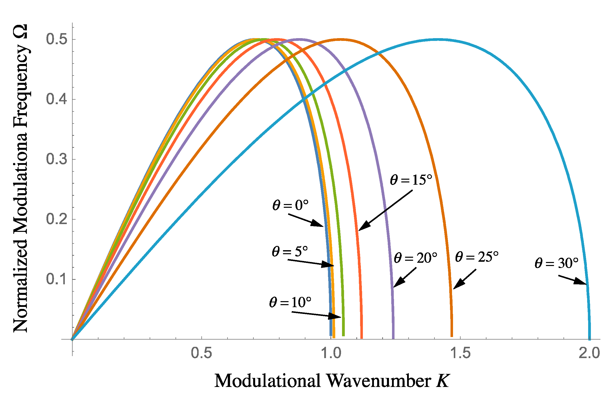
3.2. The Modulational Dispersion Relation
3.3. Goals of This and Future Papers
4. The Nonlinear Spectrum of Two-Dimensional Wave Trains
4.1. Plane Wave Solutions of the 2+1 NLS Equation
| Fact: All solutions of the 1+1 NLS equation are also plane wave solutions of the 2+1 NLS equation. |
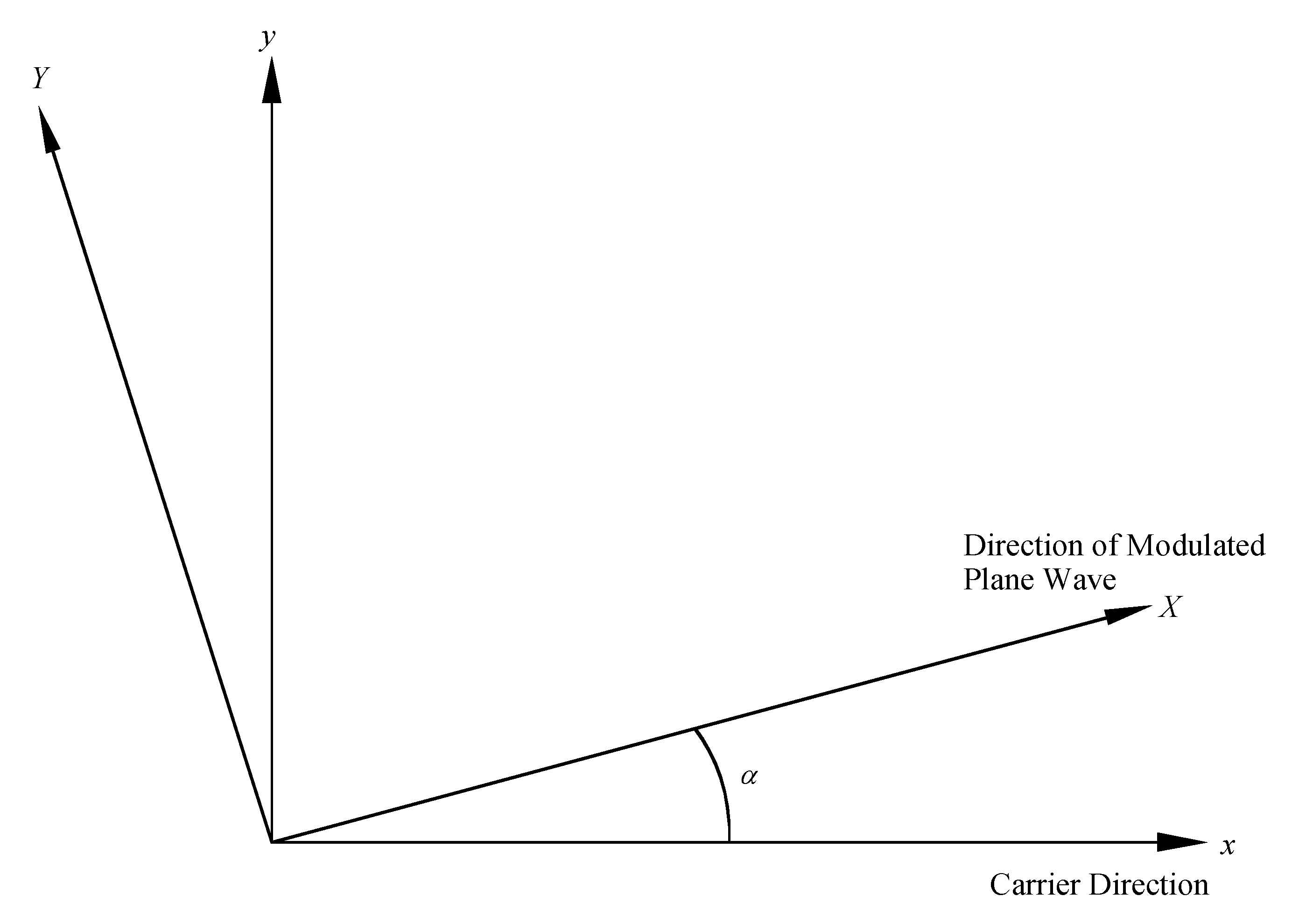
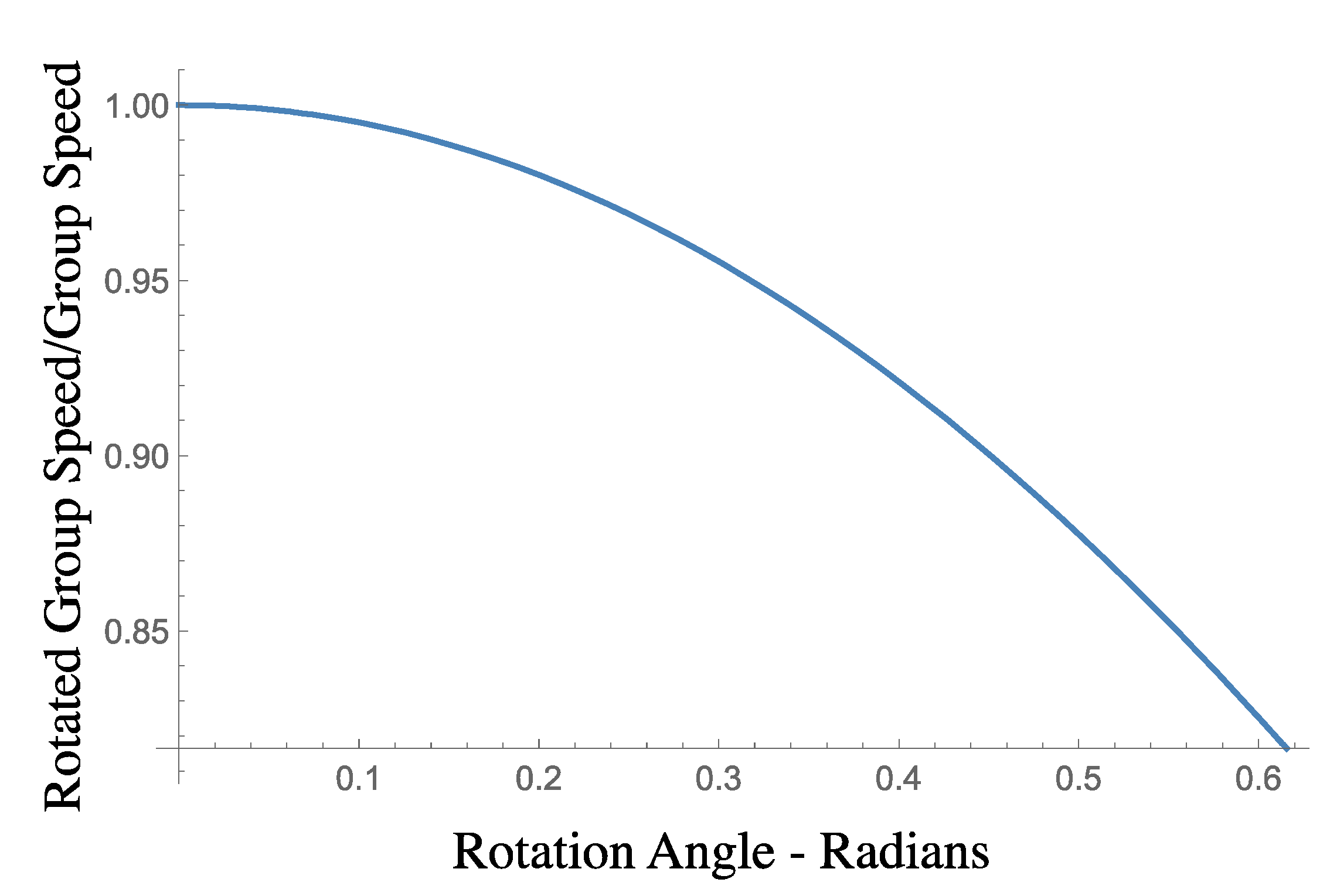
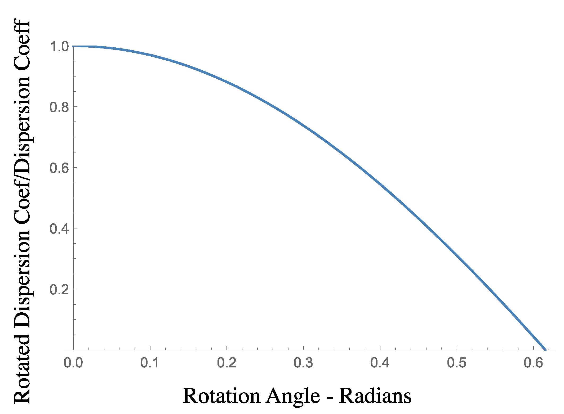
4.2. Modulation Dispersion Relation and Nonlinearity with Rotation
5. Constructing Asymptotic Solutions of the Two-Dimensional Schrödinger Equation
5.1. NLS in 2+1 Dimensions
5.2. Computing the 2+1 NLS Equation Asymptotic Solutions Using Riemann Theta Functions
5.3. Generalize the 2+1 NLS Equation to an Arbitrary Potential: The Hirota Method
5.4. Computation of the Nonlinear Spectrum in Terms of the Riemann Matrix
5.5. Riemann Spectrum for the 1+1 NLS Equation
5.6. Riemann Spectrum for the 2+1 NLS Equation
6. The Physics of the NLFA Formulation
6.1. Overview of the Formulation
6.2. A Simple Example for a Single Degree of Freedom
7. Numerical Methods of Nonlinear Fourier Analysis
7.1. Overview of Numerical Methods for Determining the Nonlinear Spectrum in 2+1 Dimensions
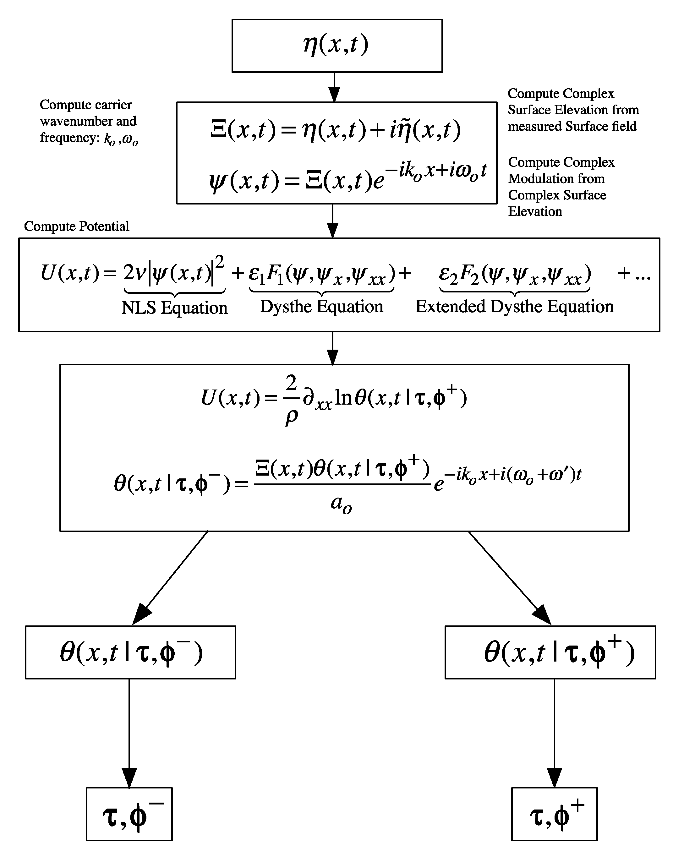
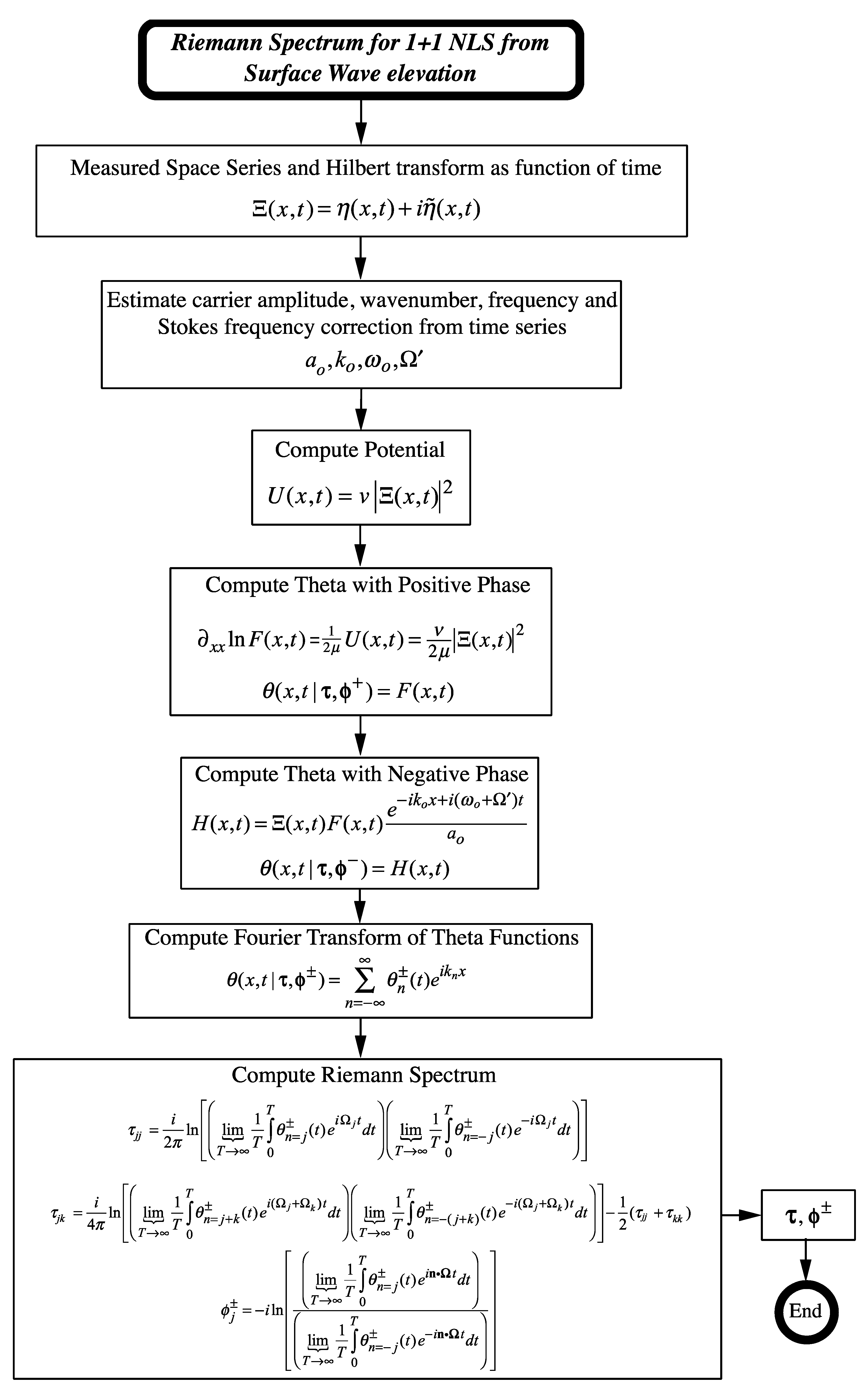
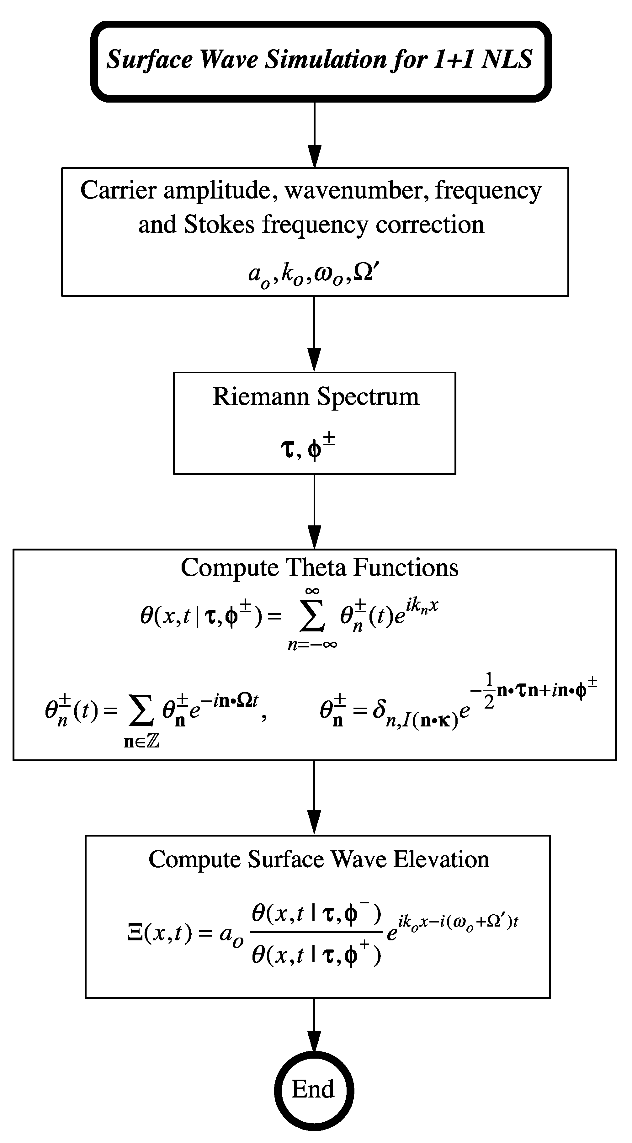
7.2. Procedure for Computing the NLFA Spectrum of the Measured Surface Wave Elevation
7.3. Interpretation of Boxed Equation (106)
- (1)
- Begin with the complex surface wave elevation , which is a rapidly oscillating function in both space and time t and from this remove the carrier oscillation together with Stokes correctionto get a slowly oscillating modulation function. This shifts the Fourier transform from the carrier wavenumber and frequency to nearly zero, just as we physically expect. This is the well-known Fourier shifting theorem at work.
- (2)
- Then, we multiply by the function , which oscillates over long spatial scales in and is slowly oscillating in t because it is a measure of the squared modulus of the surface wave elevation via (106).
- (3)
- We now have the function that also has long spatial scales and slowly varying time t.
- (4)
- Because and are long in and slow in time t, they are “theta function like” and therefore good for describing the envelope function where and .
7.4. Quasiperiodic Fourier Structure of Measured Riemann Theta Functions
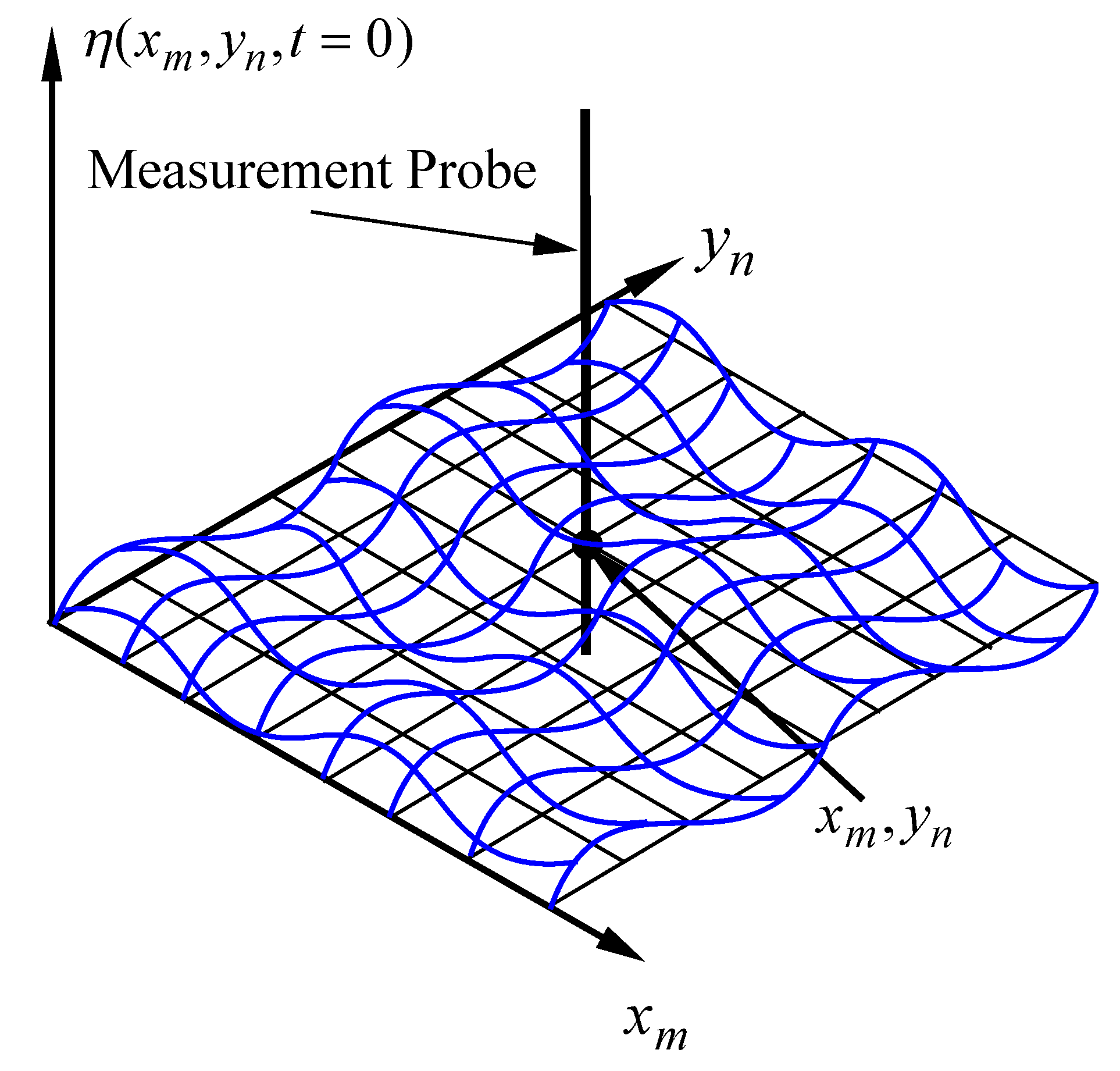
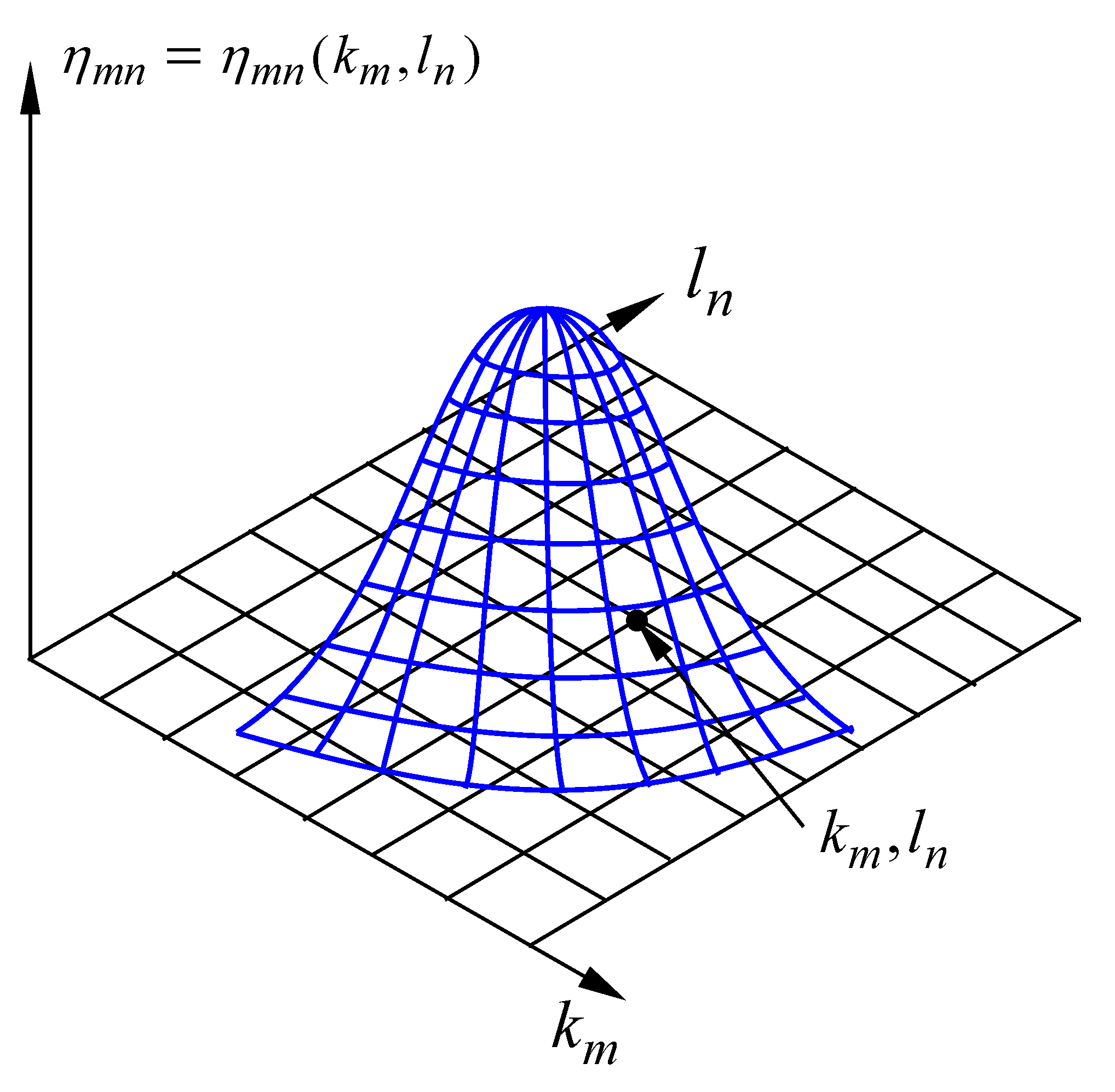
7.5. Numerical Analysis in Two Dimensions: Measurement of a Wave Field of the Sea Surface at
7.6. Numerical Analysis for a 1D Sea Surface Elevation
7.7. Concrete Example for a Single Degree of Freedom
7.8. Alternative General Notation
7.9. Primer on Nonlinear Fourier Analysis as a Theory of Nonlinearly Interacting Stokes Waves
7.10. Modeling the Surface Wave Elevation
7.11. Computing the Frequencies for Time Series Analysis and Modeling
7.11.1. The Linear Model
7.11.2. Linear Schrödinger Equation in 1+1 Dimensions
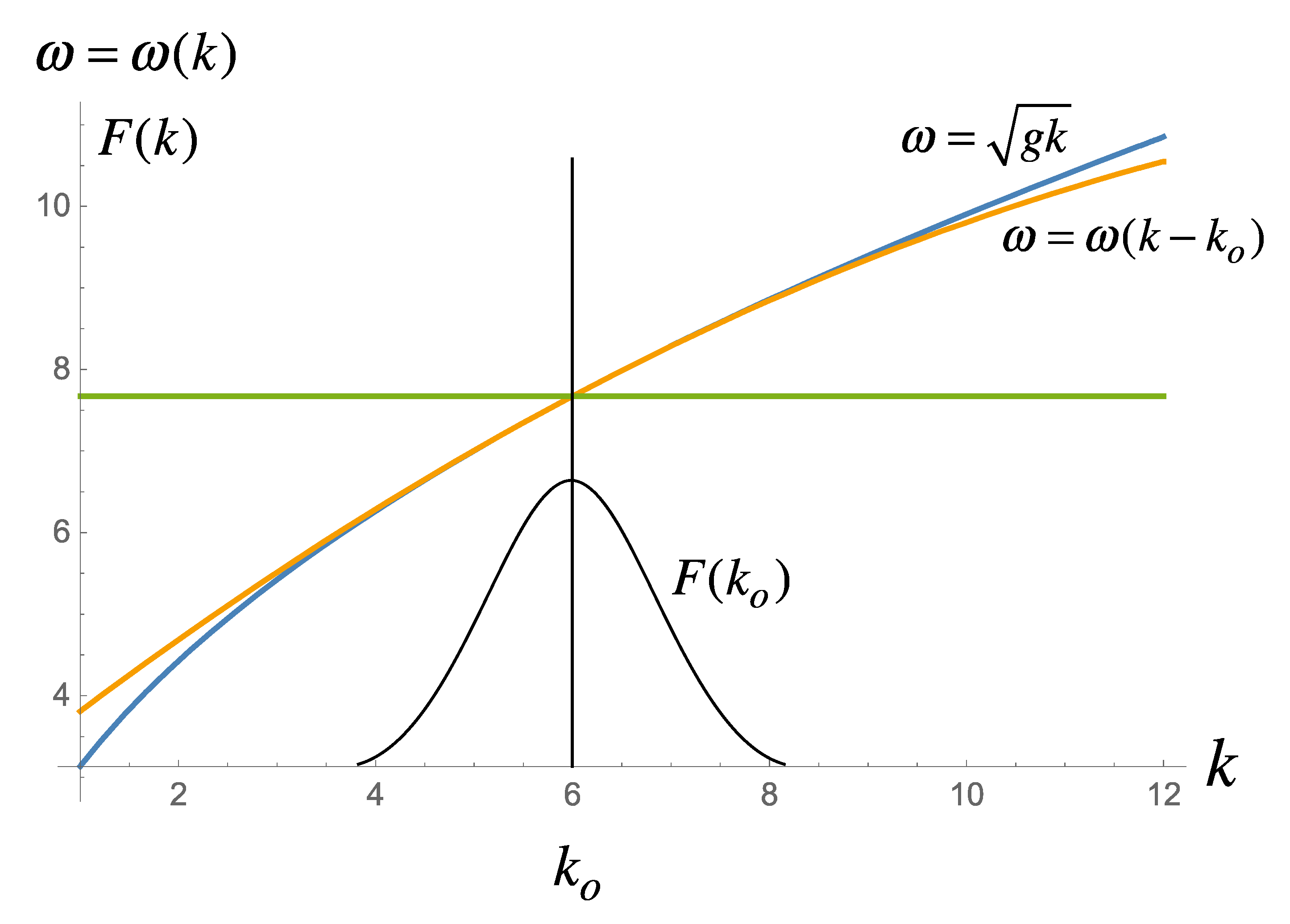
7.11.3. The Modulational Instability for 1+1 NLS
7.11.4. LSE in 2+1 Dimensions
7.11.5. The Modulational Instability in 2D
8. Application to Analysis of SINTEF Wave Tank Data
9. Application to Analysis of Wave Data in Currituck Sound
10. Application to Radar Data Assimilation and Modeling, and Real-Time Prediction of Ocean Waves
11. Summary and Discussion
Funding
Acknowledgments
Conflicts of Interest
Appendix A. What is Fourier or Harmonic Analysis?
- 1:.
- Standard Periodic Fourier Analysis
- 2:.
- Quasiperiodic Fourier Series
- 3:.
- Almost Periodic Fourier Series

| Fourier Method | Wavenumber/Frequency | Number of Spectral Components |
|---|---|---|
| Periodic Fourier Series | Commensurable/Incommensurable | Non-denumerable |
| Quasiperiodic Fourier Series | Incommensurable/Incommensurable | Denumerable |
| Almost Periodic Fourier Series | Incommensurable/Incommensurable | Non-denumerable |
References
- Osborne, A.R. Nonlinear Ocean Waves and the Inverse Scattering Transform; Academic Press: Boston, MA, USA, 2010; 976p. [Google Scholar]
- Osborne, A.R. Nonlinear Fourier methods for ocean waves. Procedia IUTAM 2018, 26, 112–123. [Google Scholar] [CrossRef]
- Osborne, A.R. Breather turbulence: Exact spectral and stochastic solutions of the nonlinear Schrödinger equation. Fluids 2019, 4, 72. [Google Scholar] [CrossRef] [Green Version]
- Osborne, A.R. Theory of Nonlinear Fourier Analysis: The Construction of Quasiperiodic Fourier Series for Nonlinear Wave Motion. In Proceedings of the ASME 2020 39th International Conference on Ocean, Offshore and Arctic Engineering OMAE2020-8536, Ft Lauderdale, FL, USA, 28 June–3 July 2020. [Google Scholar]
- Osborne, A.R.; Resio, D.T.; Costa, A.; Ponce de León, S.; Chrivì, E. Highly nonlinear wind waves in Currituck Sound: Dense breather turbulence in random ocean waves. Ocean Dyn. 2018, 69, 187–219. [Google Scholar] [CrossRef]
- Samoilenko, A.M. Elements of the Mathematical Theory of Multi-Frequency Oscillations; Kluwer Academic Publishers: Dordrecht, The Netherlands, 1991. [Google Scholar]
- Corduneanu, C. Almost Periodic Oscillations and Waves; Springer: New York, NY, USA, 2009. [Google Scholar]
- Delaunay, C. Théorie du Mouvement de la Lune; T. T. Malet-Bachelier: Paris, France, 1860. [Google Scholar]
- Poincaré, H. Periodic and Asymptotic Solutions; American Institute of Physics: University Park, MD, USA, 1993; Volume 1. [Google Scholar]
- Poincaré, H. Approximations by Series; American Institute of Physics: University Park, MD, USA, 1993; Volume 2. [Google Scholar]
- Poincaré, H. Integral Invariants and Asymptotic Properties of Certain Solutions; American Institute of Physics: University Park, MD, USA, 1993; Volume 3. [Google Scholar]
- Kolmogorov, A.N. On the Preservation of Conditionally Periodic Motions Under a Small Change of the Hamiltonian. Dokl. Akad. Nauk SSSR 1954, 98, 527–530. [Google Scholar]
- Arnol’d, V.I. Small Denominators I: On the Mappings of a Circle onto Itself. Izv. Akad. Nauk Ser. Mat. 1961, 25, 21–86. [Google Scholar]
- Arnol’d, V.I. Small Denominators: A Proof of A.N. Kolmogorov’s Theorem on Conservation of Conditionally Periodic Motions Under a Small Change of the Hamiltonian. Uspekhi Mat. Nauk 1963, 18, 13–40. [Google Scholar]
- Arnol’d, V.I. Small Denominators and the Stability Problem in Classical and Celestial Mechanics. Uspekhi Mat. Nauk 1963, 18, 91–192. [Google Scholar] [CrossRef]
- Baker, H.F. An Introduction to the Theory of Multiply Periodic Functions; Cambridge University Press: Cambridge, UK, 1907. [Google Scholar]
- Mumford, D. Tata Lectures on Theta I; Birkhäuser: Boston, MA, USA, 1982. [Google Scholar]
- Mumford, D. Tata Lectures on Theta II; Birkhäuser: Boston, MA, USA, 1984. [Google Scholar]
- Kotljarov, V.P.; Its, A.R. Explicit formulas for solutions of the Schrödinger nonlinear equation. Doklady. Akad. Nauk. Ukr SSSR. 1976, 11, 965–968. (In Ukranian) [Google Scholar]
- Previato, E. Hyperelliptic Quasiperiodic and Soliton Solutions of the Nonlinear Schrödinger Equation. Duke Math. J. 1985, 52, 320–377. [Google Scholar] [CrossRef]
- Tracy, E.R.; Chen, H.H. Nonlinear Self-modulation: An Exactly Solvable Model. Phys. Rev. A 1988, 37, 815–839. [Google Scholar] [CrossRef]
- Bohl, P. Ueber die Darstellung von Funktionen einer Variabeln Durch Trigonometrische Reihen mit Mehreren einer Variablen Proportionalen Argumenten. Ph.D. Thesis, Universitat zu Dorpat, Dorpat, Estonia, 1893; 31p. [Google Scholar]
- Bohr, H. Almost Periodic Functions; Chelsea Publishing Company: New York, NY, USA, 1947. [Google Scholar]
- Besicovitch, A.S. Almost Periodic Functions; Cambridge University Press: Cambridge, UK, 1932. [Google Scholar]
- Bochner, S. Beitraege zur Theorie der Fastperiodischen Funktionen, I. Teil: Funktionen Einer Variablen. Math. Ann. Bd. 1927, 96, 119–147. [Google Scholar] [CrossRef]
- Bochner, S. Beitraege zur Theorie der Fastperiodischen Funktionen, II. Teil: Funktionen Mehrere Variablen. Math. Ann. Bd. 1927, 96, 383–409. [Google Scholar] [CrossRef]
- Jessen, B. Bidrag Til Integralteorien for Funktioner af Uendelig Mange Variable; Habilitationsschrift: Kopenhagen, Denmark, 1930. [Google Scholar]
- Belokolos, E.D.; Bobenko, A.I.; Enol’skii, V.Z.; Its, A.R.; Matveev, V.B. Algebro-Geometric Approach to Nonlinear Integrable Equations; Springer: New York, NY, USA, 1994. [Google Scholar]
- Eliasson, L.H.; Kuksin, S.B.; Marmi, S.; Yoccoz, J.-C. Dynamical Systems and Small Divisors; Springer: Berlin, Germany, 2002. [Google Scholar]
- Dysthe, K.B. Note on a modification to the nonlinear Schrödinger equation for application to deep water waves. Proc. R. Soc. Lond. A 1979, 369, 105–114. [Google Scholar]
- Trulsen, K.; Dysthe, K.B. A modified nonlinear Schrödinger equation for broader bandwidth gravity waves on deep water. Wave Motion 1996, 24, 281–289. [Google Scholar] [CrossRef]
- Zakharov, V.E. Stability of periodic waves of finite amplitude on the surface of a deep fluid. J. Appl. Mech. Tech. Phys. USSR 1968, 2, 190. [Google Scholar] [CrossRef]
- Zakharov, V.E.; Kuznetsov, E.A. Multi-scale expansions in the theory of systems integrable by the inverse scattering transform. In Solitons and Coherent Structures; Campbell, D.K., Newell, A.C., Schrieffer, R.J., Segur, H., Eds.; North-Holland: Amsterdam, The Netherlands, 1986; pp. 455–463. [Google Scholar]
- Kimmoun, O.; Hsu, H.C.; Kibler, B.; Chabchoub, A. Nonconservative higher-order hydrodynamics modulation instability. Phys. Rev. 2017, 96, 022219. [Google Scholar] [CrossRef] [Green Version]
- Barber, N.F.; Ursell, F.; Darbyshire, J.; Tucker, M.J. A frequency analyser used in the study of ocean waves. Nature Lond. 1946, 158, 329–332. [Google Scholar] [CrossRef]
- Longuet-Higgins, M.S.; Barber, N.F. Four Theoretical Notes on the Estimation of Sea Conditions; Report N 1-N4 103.30/W; Admiralty Research Laboratory: Teddington, UK, 1946; (unpublished). [Google Scholar]
- Longuet-Higgins, M.S. The directional spectrum of ocean waves and processes of wave generation. Proc. R. Soc. Lond. A 1962, 265, 286–315. [Google Scholar]
- Longuet-Higgins, M.S. On the Nonlinear Transfer of Energy in the Peak of a Gravity-wave Spectrum: A Simplified Model. Proc. R. Soc. Long. A 1976, 347, 311–328. [Google Scholar]
- Paley, R.C.; Weiner, N. Fourier Transform in the Complex Domain; American Mathematical Society Colloquium Publications: New York, NY, USA, 1934; Volume XIX. [Google Scholar]
- Benjamin, T.B.; Feir, J.E. The disintegration of wave trains on deep water. Part 1. J. Fluid Mech. 1967, 27, 417430. [Google Scholar] [CrossRef]
- Longuet-Higgins, M.S. The statistical analysis of a random, moving surface. Phil. Trans. Roy. Soc. Lond. 1957, 249, 321–387. [Google Scholar]
- Doob, J.L. Stochastic Processes; John Wiley: New York, NY, USA, 1952. [Google Scholar]
- Papoulis, A. Probability, Random Variables and Stochastic Processes; McGraw-Hill: New York, NY, USA, 1965. [Google Scholar]
- Khintchine, A. Korrelationstheorie der stationaeren stochastischen Prozesse. Math. Ann. 1934, 109, 604–615. [Google Scholar] [CrossRef]
- Rice, S.O. The mathematical analysis of random noise. Bell Syst. Tech. J. 1944, 23, 282–332. Bell Syst. Tech. J. 1945, 24, 46–156. [Google Scholar] [CrossRef]
- Saffman, P.G.; Yuen, H.C. Stability of a plane soliton to infinitesimal two-dimensional perturbations. Phys. Fluids 1978, 8, 1450–1451. [Google Scholar] [CrossRef]
- Yuen, H.C.; Lake, B.M. Nonlinear dynamics of deep-water gravity waves. Adv. Appl. Mech. 1982, 2, 67–229. [Google Scholar]
- Hasimoto, H.; Ono, H. Nonlinear Modulation of Gravity Waves. J. Phys. Soc. Jpn. 1972, 33, 805–811. [Google Scholar] [CrossRef]
- Mei, C.C. The Applied Dynamics of Ocean Surface Waves; John Wiley and Sons: New York, NY, USA, 1983. [Google Scholar]
- Hasselmann, K. On the non-linear transfer in a gravity wave spectrum, Part 3. Evaluation of energy flux and sea-swell interactions for a Neumann spectrum. J. Fluid Mech. 1963, 15, 385–398. [Google Scholar] [CrossRef]
- Phillips, O.M. On the generation of waves by turbulent wind. J. Fluid Mech. 1957, 2, 417–445. [Google Scholar] [CrossRef]
- Young, I.R.; Verhagen, L.A.; Banner, M.L. A note on the bimodal directional spreading of fetch-limited wind waves. J. Geophys. Res. 1995, 100, 773–778. [Google Scholar] [CrossRef]
- Ewans, K.C. Observations of the directional spectrum of fetch-limited waves. J. Phys. Oceanogr. 1998, 28, 495–512. [Google Scholar] [CrossRef]
- Hwang, P.A.; Wang, D.W.; Walsh, E.J.; Krabill, W.B.; Swift, R.N. Airborne Measurements of the Wavenumber Spectra of Ocean Surface Waves. Part II: Direction Distribution. J. Phys. Ocean. 2000, 30, 2768–2787. [Google Scholar] [CrossRef]
- Long, C.E.; Resio, D.T. Wind wave spectral observations in Currituck Sound, North Carolina. J. Geophys. Res. Ocean. 2007, 112, 1–21. [Google Scholar] [CrossRef] [Green Version]
- Komen, G.J.; Cavaleri, L.; Donelan, M.; Hasselmann, K.; Hasselmann, S.; Janssen, P.A.E.M. Dynamics and Modelling of Ocean Waves; Cambridge University Press: Cambridge, UK, 1994. [Google Scholar]
- Chabchoub, A.; Mozumi, K.; Hoffmann, N.; Babanin, A.V.; Toffoli, A.; Steer, J.N.; van den Bremer, T.S.; Akhmediev, N.; Onorato, M.; Waseda, T. Directional soliton and breather beams. Proc. Nat. Acad. Sci. USA 2019, 116, 9759–9763. [Google Scholar] [CrossRef] [PubMed] [Green Version]
- Matsutani, S. Hyperelliptic Solutions of KdV and KP equations: Reevaluation of Baker’s Study on Hyperelliptic Sigma Functions. J. Phys. A Gen. Phys. 2000, 34, 4721. [Google Scholar] [CrossRef]
- Kharif, C.; Pelinovsky, E.; Slunyaev, A. Rogue Waves in the Ocean; Springer: Berlin, Germany, 2008. [Google Scholar]
- Whitham, G.B. Linear and Nonlinear Waves; John Wiley: New York, NY, USA, 1974. [Google Scholar]
- Sutherland, P.; Melville, W.K. Field measurements and scaling of ocean surface wave-breaking statistics. Geophys. Res. Lett. 2015, 40, 3074–3079. [Google Scholar] [CrossRef]
- Sutherland, P.; Melville, W.K. Measuring turbulent kinetic energy dissipation at a wavy sea surface. J. Atmos. Ocean. Technol. 2015, 32, 1498–1514. [Google Scholar] [CrossRef]
- Sutherland, P.; Melville, W.K. Field measurement of surface and near-surface turbulence in the presence of breaking waves. J. Phys. Ocean. 2015, 45, 943–965. [Google Scholar] [CrossRef]
- Cheng, H.-Y.; Chien, H. Implementation of S-band marine radar for surface wave measurement under precipitation. Remote Sens. Environ. 2017, 188, 85–94. [Google Scholar] [CrossRef]
- Lund, B.; Collins, C.O.; Graber, H.C.; Terrill, E.; Herbers, T.H.C. Marine radar ocean wave retrieval’s dependency on range and azimuth. Ocean Dyn. 2014, 64, 999–1018. [Google Scholar] [CrossRef]
- Gudmestad, O.T. Modelling of waves for the Design of Offshore Structures. J. Mar. Sci. Eng. 2020, 8, 293. [Google Scholar] [CrossRef] [Green Version]
- Fourier, J.J. Théorie Analytique de la Chaleur; Firmin Didot Père et Fils: Paris, France, 1822. [Google Scholar]
- Zygmund, A. Trigonometric Series; Cambridge University Press: Cambridge, UK, 1932. [Google Scholar]


Publisher’s Note: MDPI stays neutral with regard to jurisdictional claims in published maps and institutional affiliations. |
© 2020 by the author. Licensee MDPI, Basel, Switzerland. This article is an open access article distributed under the terms and conditions of the Creative Commons Attribution (CC BY) license (http://creativecommons.org/licenses/by/4.0/).
Share and Cite
Osborne, A.R. Nonlinear Fourier Analysis: Rogue Waves in Numerical Modeling and Data Analysis. J. Mar. Sci. Eng. 2020, 8, 1005. https://doi.org/10.3390/jmse8121005
Osborne AR. Nonlinear Fourier Analysis: Rogue Waves in Numerical Modeling and Data Analysis. Journal of Marine Science and Engineering. 2020; 8(12):1005. https://doi.org/10.3390/jmse8121005
Chicago/Turabian StyleOsborne, Alfred R. 2020. "Nonlinear Fourier Analysis: Rogue Waves in Numerical Modeling and Data Analysis" Journal of Marine Science and Engineering 8, no. 12: 1005. https://doi.org/10.3390/jmse8121005