Accurate Depth Inversion Method for Coastal Bathymetry: Introduction of Water Wave High-Order Dispersion Relation

Abstract

This paper proposes a wave model for the depth inversion of sea bathymetry based on a new high-order dispersion relation which is more suitable for intermediate water depth. The core of this model, a high-order dispersion relation is derived in this paper. First of all, new formulations of wave over generally varying seabed topography are derived using Fredholm’s alternative theorem (FAT). In the new formulations, the governing equation is coupled with wave number and varying seabed effects. A new high-order dispersion relation can be obtained from the coupling equation. It is worth mentioning that both the slope square and curvature terms (${(\nabla h)}^2,{\nabla }^{2}h,{(\nabla k)}^2,{\nabla }^{2}k,\nabla h\cdot \nabla k$) of water wavenumber and seabed bottom are explicitly expressed in high-order dispersion relation. Therefore, the proposed method of coastal bathymetry reversion using the higher-order dispersion relation model is more accurate, efficient, and economic.

1. Introduction

In coastal engineering, real-time updated and accurate water depth data are critical to solve many marine problems [1,2,3,4,5,6,7]. Traditionally, marine bathymetry data are mainly obtained by using sonar to carry out field exploration. Usually, the sonar equipment and the positioning system are installed in the measuring ship. The mesh point is arranged in the sounding water area for measurement, and the data processing is performed later. This field measurement is not only costly to operate, but also takes long duration. Due to the limitation of the regional environment, some areas cannot be measured, resulting in the lack of water depth data in these areas [8]. In addition, the ship survey is greatly affected by the weather conditions. Since traditional measurement methods have so many limitations, it is urgent to explore alternative methods.

With the development of aerial photography technology, radar and remote sensing technology, satellite derived bathymetry (SDB) is being adopted as a cheaper and more spatially extensive method for bathymetric mapping than traditional acoustic surveys [9,10,11]. However, the acquisition of depth information is affected by chlorophytes, suspended sediment, dissolved organic matter in air colour and other information in water. Therefore, in water areas with large interference from human activities and muddy water, extremely high requirements are put forward for the spectral analysis of remote sensing [12]. In other words, when the visibility of water is limited, it will lead to low accuracy in field measurements.

Although the method of coastal bathymetry by remote sensing and other technologies has many limitations, it cannot be abandoned due to its large coverage area and low budget. An interdisciplinary approach is the analysis of coastal gravity waves observed on high resolution satellite imagery over ocean which provides us with quantitative methods for estimating depth in shallow parts of the sea [13]. For instance, based on the dispersion relation and linear wave hypothesis under shallow water conditions, the bathymetry inversion system cBathy has combined an imaging technique with remote sensing, UAV (Unmanned Aerial Vehicle) systems, or GIS (Geographic Information System) to obtain the parameters needed for bathymetry inversion [14,15,16,17,18,19]. At the beginning, aerial photography, radar, or remote sensing technology are used to obtain the spatial-time sequence digital image or video image of the surface wave in the target sea area [14,18]. The acquired digital image of the sea surface or video image is identified and analyzed to obtain the wave distribution information, which is substituted into the dispersion relation model to calculate the water depth. This bathymetric technique can not only overcome the low accuracy caused by the water environment, but also obtain the water depth of the target sea area with a wide coverage in real time at a low cost. Therefore, the method mentioned above has obvious advantages compared with traditional measurement technologies.

However, the accuracy of depth inversion is directly dependent on the knowledge of a good functional dispersion relation [20]. The wave field models used in the above methods are linear dispersion relation (${\omega }^2=gk\tanh (kh)$), but this type of model has some trouble with the bar crest area, such as cBathy which is known to have higher error over the inner bar [21,22]. Tang has shown that the dispersion relation of the wave model should be used for a wide range of water depths and wave conditions [23]. Ma and Dong have indicated that the slope effect should be considered when the bottom slope is larger than 1/30 to obtain a better estimation of wave parameters [24,25].

In order to improve the accuracy of the water depth inversion, some water wave models have introduced the wave height when using the linear dispersion relation in shallow water [11,14,16]. Utilizing the slope parameter can also define the dispersion relation accurately [26]. Ehrenmark proposed a wave dispersion relation that only considers the slope of seabed topography [27]. Beji introduced an empirical correction function to improve the explicit approximation of the linear dispersion relationship for gravity waves [28].

Furthermore, as Zhang et al. have indicated that the mild-slope model (the linear dispersion relation) is not uniform for all frequencies of waves, and especially in the low frequency range, the errors induced by neglecting the additional curvature terms become large [29]. It is worth mentioning that the influence of seabed topography on the model is more obvious in the intermediate water depth. Water wave resonance can be quite varied and complex, depending on the bottom topographies [30,31]. Motivated by Yu and Howard’s research, a new high-order dispersion relation is proposed using the coupling equation in this paper, which contains the nonlinear relation of wave number caused by the change of seabed slope and curvature [32].

This paper is structured as follows. In Section 2 wave potential and the wavenumber coupling equation over general varying seabed topography are derived based on the Fredholm’s alternative theorem (FAT). A new high-order dispersion relation including ${(\nabla h)}^2,{\nabla }^{2}h,{(\nabla k)}^2,{\nabla }^{2}k,\nabla h\cdot \nabla k$ is obtained from the real part of the coupling equation. In Section 3, the numerical results of the coupling model are presented, which show that the simulated results of the single sinusoidal seabed agree with the experimental values very well. This verification can be used to prove that the high-order dispersion relation has higher accuracy than the linear dispersion relation. In Section 4, a future research topic is envisaged, and a set of bathymetry inversion models with high precision are preconceived by using high-order dispersion relation. Finally, conclusions are drawn in Section 5.

2. Wavenumber Coupling Equation and High-Order Dispersion Relation

For a small-amplitude wave with angular frequency $\omega$, it is assumed that the flow is incompressible and irrotational and the pressure is constant at the free surface. The rectilinear coordinates (x, y, z) are fixed in space and z = 0 is located at the calm water level. The wave potential $\mathsf{\Phi }(x,y,z,t)$ must satisfy the following equation and boundary conditions:

$${\nabla }^2\mathsf{\Phi }+{\mathsf{\Phi }}_{zz}=0,(-\mathrm{h}\le \mathrm{z}\le 0),$$

(1)

$${\mathsf{\Phi }}_{tt}+g{\mathsf{\Phi }}_z=0,\mathrm{at}z=0,$$

(2)

$${\mathsf{\Phi }}_z+\nabla h\cdot \nabla \mathsf{\Phi }=0,\mathrm{at}z=-h.$$

(3)

where ∇ represents the horizontal gradient operator, example:$\nabla =\left(\frac{\partial }{\partial \mathrm{x}},\frac{\partial }{\partial \mathrm{y}}\right)$.

2.1. Fredholm’s Alternative Theorem (FAT)

Fredholm’s alternative theorem (FAT) [33] is introduced in this section and briefly described as follows. Mathematically, a non-homogeneous problem can be solved whenever the corresponding homogeneous problem has unique trivial solution. However, in the alternate case, when uniqueness fails, it is solvable if and only if certain orthogonality conditions are satisfied. In other words, if the homogeneous equation has a non-trivial solution, then the corresponding non-homogeneous equation has a solution if and only if the orthogonality condition is satisfied. This theory is referred to as FAT (Fredholm’s alternative theorem).

Introduce a differential operator $\tilde{L}$ and its adjoint $\tilde{N}$, acting on function ${\varphi }_1$ and ${\varphi }_2$, respectively. Rewrite equation of Friedman as defined as

$${\displaystyle {\int }_{z_1}^{z_2}\left({\varphi }_1\tilde{L}{\varphi }_2-{\varphi }_2\tilde{N}{\varphi }_1\right)}\mathrm{d}z={J\left({\varphi }_1,{\varphi }_2\right)|}_{z_1}^{z_2},$$

(4)

where $\tilde{L}{\varphi }_2=\frac{{\partial }^2{\varphi }_2}{\partial z^2}$ and $\tilde{N}{\varphi }_1=\frac{{\partial }^2{\varphi }_1}{\partial z^2}$ Friedman indicated that $z_1$ and $z_2$ are arbitrary constants [33]. And $\mathrm{J}\left({\varphi }_1,{\varphi }_2\right)$ is the conjunct of the functions ${\varphi }_1$ and ${\varphi }_2$, defined as

$$\mathrm{J}\left({\varphi }_1,{\varphi }_2\right)={\varphi }_1\frac{\partial {\varphi }_2}{\partial z}-{\varphi }_2\frac{\partial {\varphi }_1}{\partial z}.$$

(5)

If $\tilde{L}$ = $\tilde{N}$, the differential is said to be formally self-adjoint. If, in addition, boundary conditions for ${\varphi }_1$ and ${\varphi }_2$ are such that the conjunct J vanishes identically, the operator is said to be Hermitian.

Considering the Laplace differential operator for water wave problems, let

$$\tilde{N}=\left(\frac{{\partial }^2}{\partial x^2},\frac{{\partial }^2}{\partial y^2}\right),\mathrm{and}\tilde{L}=\frac{{\partial }^2}{\partial z^2},$$

(6)

thus, the Laplace Equation (1) can be re-written as:

$$\tilde{L}\mathsf{\Phi }=\frac{{\partial }^2\mathsf{\Phi }}{\partial z^2}=-\tilde{N}\mathsf{\Phi }=-{\nabla }^2\mathsf{\Phi },(-\mathrm{h}\le \mathrm{z}\le 0).$$

(7)

Since the operator $\tilde{N}$ commutes with the operator $\tilde{L}$, we may treat $\tilde{N}$ as a constant in the process of dealing with operator $\tilde{L}$. In other words, Equation (1) will be first considered as an ordinary differential equation for function of z, together with boundary conditions.

For the water wave problem, the operator $\tilde{L}$ is only formally self-adjoint, i.e., $\tilde{N}$ = $\tilde{L}$, but not Hermitian due to the non-homogeneous boundary conditions at free surface and bottom. $z_1$ and $z_2$ are defined as water surface and seabed, respectively. Applying the FAT to the homogeneous and non-homogeneous solutions of the wave problem, i.e., substituting ${\varphi }_1$ and ${\varphi }_2$ to be solved, the orthogonality condition for waves over a varying bottom can be obtained

$${\displaystyle {\int }_{-\mathrm{h}}^0\left[{\varphi }_1\frac{{\partial }^2{\varphi }_2}{\partial z^2}-{\varphi }_2\frac{{\partial }^2{\varphi }_1}{\partial z^2}\right]}\mathrm{dZ}={J\left({\varphi }_1,{\varphi }_2\right)|}_{Z=-h}^{Z=0}.$$

(8)

Assuming that both ${\varphi }_1$ and ${\varphi }_2$ are Lebesgue square integrable, this theorem is valid for arbitrary boundary conditions. For water wave problems, both non-homogeneous boundary conditions on the free surface and bottom will be applicable. However, if the functions are not square integrable, the Fredholm alternative theorem can be extended to such cases as Garabedian indicated [34].

2.2. Wavenumber and Velocity Potential Coupling Equation

Assume that the velocity potential has the following form of variable separation:

$$\mathsf{\Phi }(x,y,z,t)=f(q,Q)\varphi (x,y,t)+\mathrm{non}-\mathrm{propagating}\mathrm{modes},$$

(9)

where $Q=k(z+h),q=kh,\sigma =\tanh (q),f=\cosh Q/\cosh q$ is the eigen-function of homogeneous solution, $\varphi (x,y,t)$ is the 2-D wave velocity potential and $\mathsf{\Phi }(x,y,z,t)$ is the 3-D wave potential. Substituting ${\varphi }_1=f\mathrm{and}{\varphi }_2=\mathsf{\Phi }$, using equation (8), we have:

$$J{(f,\mathsf{\Phi })}_{z=0}-J{(f,\mathsf{\Phi })}_{z=-h}+{\displaystyle {\int }_{-h}^0\left(f{\nabla }^2\mathsf{\Phi }+\mathsf{\Phi }\frac{{\partial }^{2}f}{\partial z^2}\right)}dz=0.$$

(10)

Substituting the linearized free surface boundary condition and the bottom boundary condition, and paying attention to $f=1\mathrm{or}1/\cosh q,\mathrm{and}{f}_z=k\tanh (q)\mathrm{and}0\mathrm{when}z=0$$\mathrm{and}z=-h$, respectively, the new coupling equation for surface waves propagating over generally varying seabed may be formulated by utilizing equations above based on FAT governing the velocity potential $\varphi$ (x, y, t) and the wavenumber k (x, y):

$${\left({\mathsf{\Phi }}_{tt}+gk\sigma {\mathsf{\Phi }}_z\right)}_{z=0}-g{\displaystyle {\int }_{-h}^0\left[f{\nabla }^2\mathsf{\Phi }+k^{2}f\mathsf{\Phi }\right]}dz-{\frac{g}{\cosh q}\nabla h\cdot \nabla \mathsf{\Phi }|}_{z=-h}=0.$$

(11)

After a long derivation of integration along the vertical direction in the above equation which is shown in the Appendix A, the time-dependent equation governing the velocity potential $\varphi (x,y,t)$ and the wave number k (x; y) is obtained:

$${\varphi }_{tt}-\nabla \cdot (P\nabla \varphi )+\left[{\omega }^2-k^{2}P-gF\right]\varphi =0,$$

(12)

where

$$\begin{array}{l}F=g\{\left(1-{\sigma }^2\right)\left(q{\sigma }^2-\sigma \right)k{(\nabla h)}^2-\frac{1}{2}q\sigma \left(1-{\sigma }^2\right){\nabla }^{2}h-\left(1-{\sigma }^2\right)\left(2\mathrm{q}{\sigma }^2-\frac{5\sigma }{2}-\frac{\mathrm{q}}{2}\right)h\nabla h\cdot \nabla k+\\ \frac{1}{4k^3}\left[q\left(1-{\sigma }^2\right)\left(4q^2{\sigma }^2-\frac{4}{3}{q}^2-2q\sigma -1\right)+\sigma \right]{(\nabla k)}^2+\frac{1}{4k^2}\left[q\left(1-{\sigma }^2\right)(1-2q\sigma )-\sigma \right]{\nabla }^{2}k\},\end{array}$$

(13)

$$P=\frac{g\left[\sigma +\left(1-{\sigma }^2\right)q\right]}{2k}.$$

(14)

The water depth variable h is the local water depth and is expressed as the function of x and y, i.e., $h(\mathrm{x},\mathrm{y})$; $\omega$ is the wave frequency, g is the gravitational acceleration and $\mathrm{k}(\mathrm{x},\mathrm{y})$ is the wave number. For simplification of derivation, σ = tanh(q) is used, where q = kh is the product of wave number and water depth. ${(\nabla h)}^2$ represents the square term of the slope of the seabed, ${\nabla }^{2}h$ represents the seabed topography curvature term, ${(\nabla k)}^2$ represents the square term of the slope of the water wave number, and ${\nabla }^{2}k$ represents the water wave number curvature term.

2.3. New High-Order Dispersion Relation Formulation

A new high-order dispersion relation can be obtained from the derived seabed wave coupling equation, and the water depth can be directly calculated under medium and small wave conditions. Let the wave velocity potential function be:

$$\varphi (\mathrm{x},\mathrm{y},\mathrm{t})=\frac{1}{2}A(x,y,t)e^{i\tilde{\theta }}+c.c,$$

(15)

where $\mathrm{A}(\mathrm{x},\mathrm{y},\mathrm{t})$ is the amplitude of $\varphi (\mathrm{x},\mathrm{y},\mathrm{t})$, while $\theta$ is the phase of $\varphi (\mathrm{x},\mathrm{y},\mathrm{t})$, which are defined by $\tilde{k}=\nabla \tilde{\theta }$, $\tilde{\omega }=-\frac{\partial \tilde{\theta }}{\partial t}$. Further, c.c is complex conjugate. The coupling equation can be decomposed into real and imaginary parts of corresponding dispersion relation and wave action conservation, respectively [35]. Thus, the real part is

$${\tilde{\omega }}^2={\omega }^2+P\left({\tilde{k}}^2-k^2\right)+\frac{A_{tt}}{A}-P\frac{{\nabla }^{2}A}{A}-\frac{\nabla \left(P\right)\cdot \nabla A}{A}-gF,$$

(16)

which leads to a new high-order dispersion relation:

$$\begin{array}{c}{\omega }^2=gk\sigma +A_{tt}/A+gk\left(1-{\sigma }^2\right)\\ \left[{\beta }_1\frac{{\nabla }^{2}A}{A{k}^2}+{\beta }_2\frac{{\nabla }^{2}h}{k}+{\beta }_3\frac{{\nabla }^{2}k}{k^3}+{\beta }_4\frac{\nabla A}{Ak}\cdot \nabla h+{\beta }_5\frac{\nabla A}{A{k}^3}\cdot \nabla k+{\beta }_6{(\nabla h)}^2+{\beta }_7\frac{{(\nabla k)}^2}{k^4}+{\beta }_8\frac{\nabla k\cdot \nabla h}{k^2}\right]\end{array},$$

(17)

where

$${\beta }_1=-\left[\sigma +q\left(1-{\sigma }^2\right)\right]/2\left(1-{\sigma }^2\right),$$

(18)

$${\beta }_2=q\sigma /2,$$

(19)

$${\beta }_3=-\left[\sigma -q\left(1-{\sigma }^2\right)(1-2q\sigma )\right]/4{\left(1-{\sigma }^2\right)}^2,$$

(20)

$${\beta }_4=-(1-q\sigma ),$$

(21)

$${\beta }_5=[\sigma -q(1-2q\sigma )]/2,$$

(22)

$${\beta }_6=\sigma (1-q\sigma ),$$

(23)

$${\beta }_7=\left[q\left(3+6q\sigma -12q^2{\sigma }^2+4q^2\right)-3\sigma \right]/12,$$

(24)

$${\beta }_8=q\left(5\sigma +q-4q{\sigma }^2\right)/2.$$

(25)

In this paper, the change of wave number comes from the change of water depth under the ideal condition of single sinusoidal topography. The equation can be recovered from the coupling equation by using the relation of the wave-number slope and curvature with those of the bottom [29], which are obtained from:

$$\frac{\nabla k}{k}={\tau }_1\frac{\nabla h}{h},$$

(26)

$$\frac{{\nabla }^{2}k}{k}={\tau }_1\frac{{\nabla }^{2}h}{h}+{\tau }_2\frac{{(\nabla h)}^2}{h^2},$$

(27)

$$\frac{\nabla A}{A}={\tau }_3\frac{\nabla h}{h},$$

(28)

$$\frac{{\nabla }^{2}A}{A}={\tau }_3\frac{{\nabla }^{2}h}{h}+{\tau }_4\frac{{(\nabla h)}^2}{h^2},$$

(29)

$${\tau }_1=\left[-q\left(1-{\sigma }^2\right)\right]/\gamma ,$$

(30)

$${\tau }_2=\left[2q^2\left(1-{\sigma }^2\right)(\gamma -\alpha )\right]/{\gamma }^2,$$

(31)

$${\tau }_3=q\alpha /{\gamma }^2,$$

(32)

$${\tau }_4=\left[q^2\left(5\alpha -2\gamma {\sigma }^2\alpha +\left(1-{\sigma }^2\right){\sigma }^2{\gamma }^2\right)\right]/{\gamma }^4,$$

(33)

$$\alpha =-\sigma q\left(1-{\sigma }^2\right)/2,$$

(34)

$$\gamma =\sigma +q\left(1-{\sigma }^2\right).$$

(35)

According to Equations (26)–(35), the change of wave number and the change of velocity potential function are proportional to the square of slope and curvature of seabed. By substituting ${\beta }_{1-8}$ and Equations (26)–(35) into Equation (17), the specific formula of the expression of the high-order dispersion relation of the seabed with varying depth is obtained as follows:

$${\omega }^2=gk\tanh (kh)-\frac{g\xi }{4}{\nabla }^{2}h+\frac{gk{\xi }^2\left[9{\sigma }^2-{\mu }_{1}q+{\mu }_2{q}^2+{\mu }_3{q}^3+{\mu }_4{q}^4\right]}{12{\eta }^3}\left[{(\nabla h)}^2\right],$$

(36)

$$\xi =1-{\sigma }^2,$$

(37)

$$\eta =\sigma +q\xi ,$$

(38)

$${\mu }_1=12\sigma +9{\sigma }^3,$$

(39)

$${\mu }_2=9+45{\sigma }^2-18{\sigma }^4,$$

(40)

$${\mu }_3=28\sigma -78{\sigma }^3+30{\sigma }^5,$$

(41)

$${\mu }_4=10-40{\sigma }^2+42{\sigma }^4-12{\sigma }^6,$$

(42)

where water depth variable h is the local water depth and is expressed as the function of x and y, i.e.,$h(\mathrm{x},\mathrm{y})$, ω is the wave frequency, g is the gravitational acceleration, and $\mathrm{k}(\mathrm{x},\mathrm{y})$ is the wave number. For simplification of the derivation, σ = tanh(q) is used, where q = kh is the product of wave number and water depth.

Finally, a new high-order dispersion relation is obtained, which contains the square of the slope terms and the curvature terms of the seabed.

3. Verification of High-Order Dispersion Relation Model

3.1. Numerical Solution Procedure

For simplicity, the two-dimensional wave problem is studied in this section. For 2-D waves in steady state $\varphi (\mathrm{x},\mathrm{y},\mathrm{t})=\mathrm{Re}\{\tilde{\varphi }(\mathrm{x},\mathrm{y})e^{-i\omega t}\}$, and the reflection coefficient Cr is calculated by $C_r=\mathrm{Re}\{\tilde{\varphi }(i)-1\}$, where the symbol Re represents the real part of a complex value [36]. The coupling equation becomes

$${\left(P{\tilde{\varphi }}_x\right)}_x+p\tilde{\varphi }=0,$$

(43)

where

$$p=k^{2}P+gF.$$

(44)

The boundary conditions for a patch of rippled beds are

$${\tilde{\varphi }}_x=-ik\left(\tilde{\varphi }-2{\tilde{\varphi }}_I\right)\left(x_1\le 0\right),$$

(45)

$${\tilde{\varphi }}_x=ik\tilde{\varphi }\left(x_2\ge L\right),$$

(46)

where ${\tilde{\varphi }}_I=e^{ikx}$ is the incident wave of unit amplitude, $x_1$ and $x_2$ represent the up-wave and down-wave limits of the computational grid, and L is the length of computation domain. These boundary conditions have been given previously by Kirby [37].

Considering potential applications in the three-dimensional wave, a FEM model is developed for general topography. The FEM model has advantages in the three-dimensional problems with complex geometries, where it is desirable to use irregular meshes.

Multiplying the entire left-hand side of Equation (43) with a weight function w, and integrating over the domain (0, L) gives the weighted-residual statement:

$${\displaystyle {\int }_0^L\left\{{\left(P{\tilde{\varphi }}_x\right)}_x+p\tilde{\varphi }\right\}}wdx=0.$$

(47)

Mathematically, the above equation is a statement that the numerical error needs to be zero in the weighted-integral sense. The trading of differentiability from $\tilde{\varphi }$ to $w$ provides the weak form

$${\displaystyle {\int }_0^L\left(P{\tilde{\varphi }}_x{w}_x-p\tilde{\varphi }w\right)}dx-{\left[Pw{\tilde{\varphi }}_x\right]|}_0^L=0.$$

(48)

The trading of differentiability from $\tilde{\varphi }$ to $w$ can only be performed if it leads to boundary terms that are physically meaningful. The choice of the approximation for weight function gives the boundary term $P{\left(\tilde{\varphi }\right)}_x\tilde{\varphi }$, which has physical meaning of energy flux through a section. It is easy to find that the primary variable and the secondary variable are $\tilde{\varphi }$ and ${\left(\tilde{\varphi }\right)}_x$ respectively. Thus ${\left[{\tilde{\varphi }}_x\right]|}_0^L$ is the natural boundary condition. Using the notation of Reddy [38], we have

$$B(w,\tilde{\varphi })-l(w)=0,$$

(49)

where

$$B(w,\tilde{\varphi })={\displaystyle {\int }_0^L\left(P{\tilde{\varphi }}_x{w}_x-p\tilde{\varphi }w\right)}dx-{[ikPw\tilde{\varphi }]|}_0^L,$$

(50)

and

$$l(w)=-{\left[2ikPw{\tilde{\varphi }}_I\right]|}_{x=0}$$

(51)

are bilinear and linear forms, respectively. Here, the bilinear form is asymmetric. For a typical element, $\tilde{\varphi }$ is approximated by

$$\tilde{\varphi }={\displaystyle \sum _{j=1}^4{\tilde{\varphi }}_j}{N}_j,$$

(52)

where $N_j$ are cubic shape functions and ${\tilde{\varphi }}_j$ are unknowns at the nodes. The water depth h(x), slope and curvature of both h and k at each element in the FEM scheme can readily be evaluated as

$$\begin{array}{l}h={\displaystyle \sum _{j=1}^4{h}_j}{N}_j,k={\displaystyle \sum _{j=1}^4{k}_j}{N}_j\\ h_x={\displaystyle \sum _{j=1}^4{h}_j}\frac{\partial N_j}{\partial x},k_x={\displaystyle \sum _{j=1}^4{k}_j}\frac{\partial N_j}{\partial x}\\ h_{xx}={\displaystyle \sum _{j=1}^4{h}_j}\frac{{\partial }^2{N}_j}{{\partial }^{2}x},k_{xx}={\displaystyle \sum _{j=1}^4{k}_j}\frac{{\partial }^2{N}_j}{{\partial }^{2}x}\end{array}$$

(53)

In the FEM schemes, Bubnov–Galerkin method is adopted, thus, the solution shape functions are used as weighting functions.

As noted by Reddy, not all differential equations admit the functional formulation, and in order for the functional to exist, the bilinear form must be symmetric in its arguments [38]. Since the weak form statement is equivalent to the differential equation and the specified natural boundary condition of the problem, the weak form FEM is used in this study.

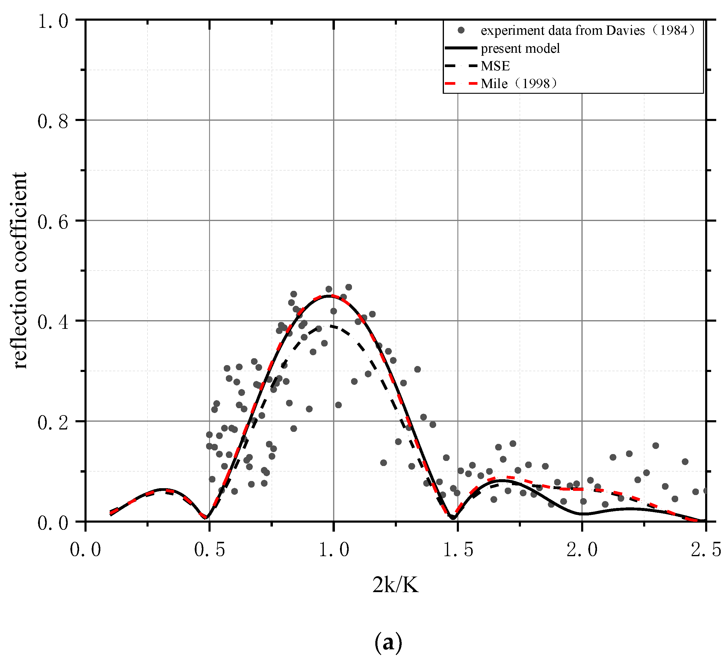
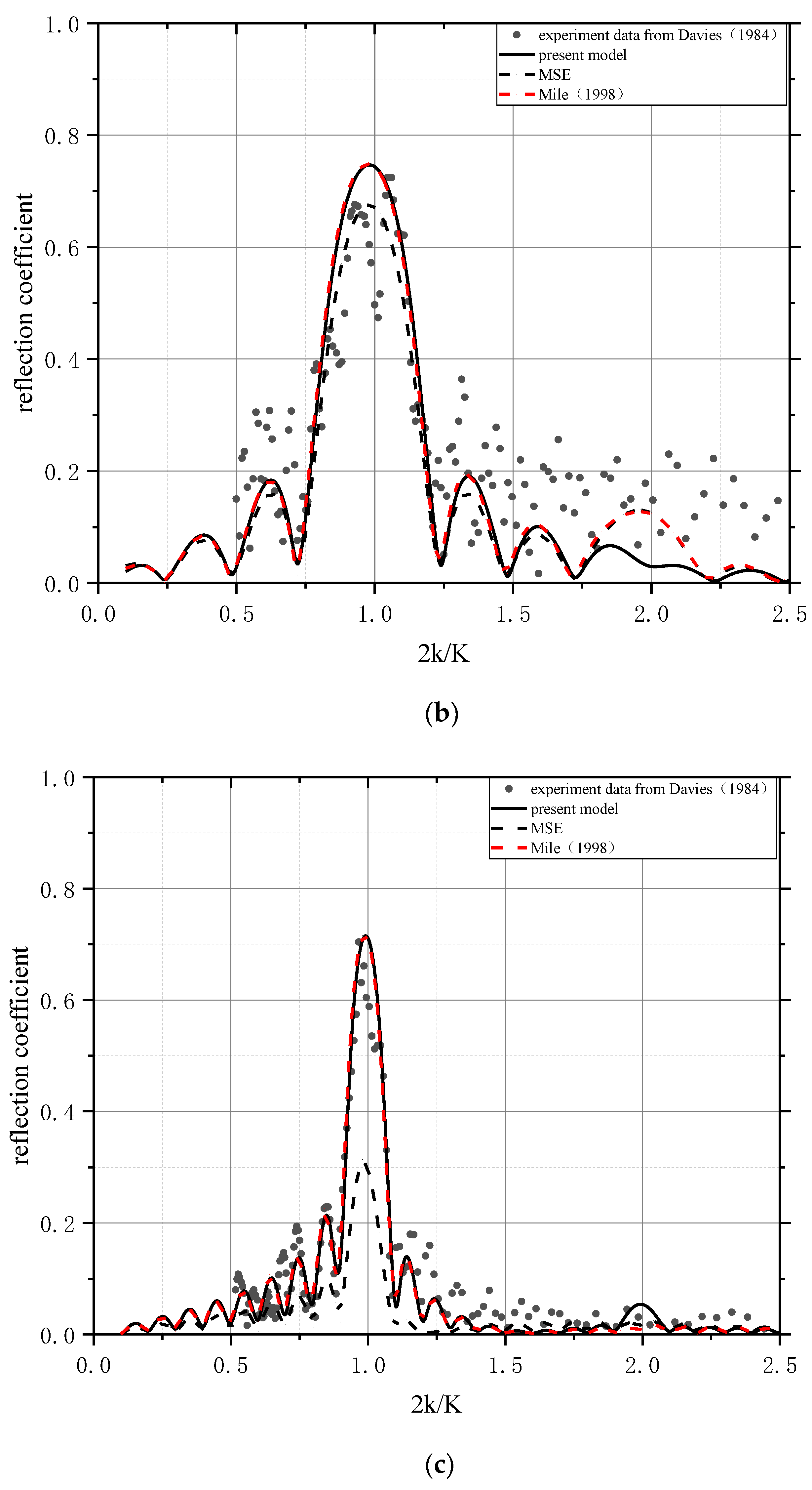
3.2. Numerical Results vs. Experiment Data

This new method of nearshore bathymetry is characterized by the nonlinear relation of wave number caused by the change in seabed slope and curvature, which is embodied in the square term of the slope and the curvature term of the seabed. In order to ensure the accuracy of the model, the numerical results are compared with the experimental values. In this paper, a type of seabed topography is selected for verification: single sinusoidal ripples.

The single sinusoidal seabed topography is expressed as follows:

$$h=\{\begin{array}{cc}{h}_0& x\le 0\\ h_0-B\sin Kx& 0<x<2\pi n/K\\ h_0& x\ge 2\pi n/K\end{array}.$$

(54)

In the two-dimensional coordinate system, the high-order dispersion relation (36) becomes:

$${\omega }^2=gk\tanh (kh)+P_1\left[{(h_x)}^2\right]+P_2{h}_{xx},$$

(55)

where

$$P_1=\frac{gk{\xi }^2\left[9{\sigma }^2-{\mu }_{1}q+{\mu }_2{q}^2+{\mu }_3{q}^3+{\mu }_4{q}^4\right]}{12{\eta }^3},$$

(56)

$$P_2=-\frac{g\xi }{4}.$$

(57)

The new high-order dispersion relation can be applied to surface waves propagating over single sinusoidal ripples. The dispersion relation is the real part of the water wave governing equation. we consider several examples pertaining to the interaction of small-amplitude monochromatic water waves with steep bottom undulations consisting of single sinusoids. Computations of wave reflection by sinusoidal beds are suitable examples to test the accuracy of the MSE and the coupling equation by comparing with experimental data from Davies and Heathershaw [39], which is equivalent in that the high-order dispersion relation is compared with the linear dispersion relation. Considering the same cases of their papers, the single sinusoidal seabed parameters are listed in

Table 1. Parameters in the experiments.

Items	(a)	(b)	(c)
number of ripples n	2	4	10
mean water depth $h_0$ (cm)	15.6	15.6	31.3
amplitude of ripples B (cm)	5	5	5
wavelength of ripples L (cm)	100	100	100

.

Figure 1a–c show the comparisons between the numerical solution and experimental value of the high-order dispersion model under three single sinusoidal bottom forms. The x-coordinate in both figures is double ratio of the wavenumber of surface to the topographic wavenumber, and the y-coordinate is the reflection coefficient of wave. The experimental data are shown as black dots which come from the classical model experiment of Davies, the dash line represents the numerical result of mild-slope equation, and the red dash line represents the numerical result of the modified mild-slope equation [40] and the solid line is the numerical result of this theory.

It can be seen that the present model and Miles and Chamberlain’s model perform exceptionally well in predicting experimental data in Figure 1a–c [40]. However, there are still differences, especially at the subpeak position. In case (a,b), Miles and Chamberlain’s model is the same as the MSE, which is closer to the experimental data. However, the two models cannot predict the trend from high to low to high of the experimental data around 2k/K = 2. In case (c), the present model shows better results when predicting the subpeak trend compared to the other two models despite a slight phase shift. In future research, we should explain the reasons for those situations, so that the present model will be closer to the experimental data.

The numerical results of the present model are presented in Figure 1a–c, which show that the simulated results of the single sinusoidal seabed agree with the experimental values very well in general. The fitting effect between the present model and laboratory is much better than that of the original mild-slope equation (MSE), which can be considered that the high-order dispersion relation is improved compared with the linear dispersion relation. It is more noteworthy that practical verification should be illustrated in future research, including comparisons with more complete models for water wave propagation over variable bathymetry, as the consistent coupled-model theory presented by Athanassoulis and Belibassakis [41].

Correlation coefficients are calculated between the numerical solutions of the high-order dispersion relation model and the experimental values in the three cases, which are shown in

Table 2. Correlation coefficients of each case.

Items	(a)	(b)	(c)
Correlation Coefficient	0.857	0.924	0.965

. The correlation coefficient $R={\displaystyle {\sum }_{i=1}^M[(S_i-\overline{S})({\mathrm{O}}_i-\overline{\mathrm{O}})]}/{[{\displaystyle {\sum }_{i=1}^M{(S_i-\overline{S})}^2}{\displaystyle {\sum }_{i=1}^M{({\mathrm{O}}_i-\overline{\mathrm{O}})}^2}]}^{1/2}$, where $S_i$ and $O_i$ denote predicted and theoretical or observed data, respectively, $\overline{S}$ and $\overline{O}$ are mean values of $S_i$ and $O_i$, and M is the number of evaluation point [42]. It can be observed that the correlation coefficients increase with the number of ripples. In other words, the high-order dispersion model is more adaptable to real undulating ocean bed forms.

In other models, it is about 0.75 of the maximum correlation coefficients between the solution generated by surface wave and seabed [42]. When considering the influence of bottom shape changes and the wave number changes caused by the topographic change, the high-order dispersion relation model shows a higher fitting degree and accuracy than the linear dispersion relation.

Table 3. Wavenumber k and wavelength L (m) calculated by linear and high-order dispersion.

	Water Depth (cm)	10.0	15.6	20.0	30.0
Linear dispersion relation	wavenumber (k)	6.802	5.675	5.183	4.576
	wavelength (L)	0.923	1.107	1.212	1.372
High-order dispersion relation	wavenumber (k)	6.697	5.679	5.424	4.639
	wavelength (L)	0.932	1.106	1.198	1.375

shows the wave number and wave wavelength (m) when the water depth (cm) is different under single sinusoidal seabed profile (the shape is consistent with case a–c) with a 1s wave period in the lab wave scale.

When the seabed profile is the same, the wavelength and wave number of the high-order dispersion relation model and linear dispersion model under different water depths are given in Table 3. When the water depth is shallow or deep, that is, the water depth is 10.0, 15.6, and 30.0 cm, the results calculated by the present dispersion relation are not much different from the wave number and wavelength. However, when the water depth is 20.0 cm, that is, at the intermediate water depth range, the accuracy difference of the high-order dispersion relation and linear dispersion relation is five times that of other water depths as mentioned above. This indicates that the high-order dispersion relation has better adaptability in the intermediate water depth. Therefore, the new high-order dispersion relation is used to calculate the intermediate water depth with higher accuracy.

Considering Equation (55), we can see that the coefficient in front of the curvature term and slope square term is a function of q. Therefore, the high-order dispersion relation mentioned above has higher accuracy in the intermediate water depth, which can be observed from Figure 2. As shown in Figure 2, the solid line represents the coefficient in front of the curvature term of seabed topography, while the dotted line represents the coefficient in front of the square of slope term of seabed topography. The bottom form is the same shape as case a–c.

It can be observed that the value of $P_1$ and $P_2$ fluctuate greatly when the value of q is in the interval (1,5). That is to say, the depth inversion has to consider the bottom topography in the intermediate because the nonlinear effect caused by terrain change on wave propagation is difficult to ignore. At the same time, it can be seen that the influence of the terrain curvature and slope square terms on the wave propagation cannot be ignore when the curvature or slope of seabed is very large. This can also explain why the error increases significantly when linear dispersion relation is used in the intermediate water depth.

4. Discussion

In this section, the future research topic will be envisaged, and a set of bathymetry inversion models with high precision is preconceived by using a high-order dispersion relation. The following is the design of the implementation steps of the water depth inversion:

Firstly, a digital image or video image of the surface-temporal sequence of waves in the target sea area can be collected from UAVs (unmanned aerial vehicle) among other ways such as radar and remote sensing.

Then, the acquired image is processed with the maximum total coherence frequency band, and the corresponding frequency and wave number pairs are generated at each calculation point [43]. For the obtained digital image or video image, the Fourier transform is used to decompose time-varying pixels and the Fourier coefficients of the time-varying pixels are further normalized. Then, select the subset of normalized Fourier coefficients around the depth location to be determined, and calculate the intersection of all pixels in the subset density spectrum. Matching wave phases are determined for each selected frequency, and generate a set of frequencies and corresponding wave numbers at each calculation point.

Finally, the obtained wave numbers and frequencies are substituted into the high-order dispersion relation model for iterative calculation to obtain the target sea depth. The final obtained depth value of the target sea area is a continuous time process. The specific implementation process is shown in Figure 3.

5. Conclusions

The resulting reflection coefficient for a single sinusoidal bottom is compared with the results of numerical solutions of the mild-slope equation and modified mild-slope equation. The present model which includes five terms (${(\nabla h)}^2,{\nabla }^{2}h,{(\nabla k)}^2,{\nabla }^{2}k,\nabla h\cdot \nabla k$) can perform exceptionally well in predicting experimental data, especially predicting the trend from high to low to high of the experimental data around the subpeak (2k/K = 2). Although the capability of this model in the weak reflection area is not good enough, in future research, more attention will be paid to this aspect to improve the accuracy of the model. A new high-order dispersion relation emerges that offers significantly increased accuracy over a single sinusoidal bottom, which is derived from the real part of the coupling equation.

We have presented a model frame that space-time sequence digital images or videos combine with high-order dispersion relation for bathymetry mapping. The high-order dispersion relation model has higher adaptability in the intermediate water depth with complex seabed, such as bed with sand bar formation etc.

The reasons why selecting a single sinusoidal seabed form for model verification can be summarized as follows:

(1) There are internationally recognized model experiments and valuable data from Davies, which are the basis of model validation.

(2) It can be widely used in practical engineering. For example, the profiles of the most artificial sand dam and submerged dike are sinusoidal.

(3) Mathematically, any seabed shape can be decomposed into sinusoidal form by the Fourier transform.

The acquisition of the space-time sequence digital images or video images of the surface wave in the target sea area is fast in time, low in cost, easy and secret to operate, eliminating the drawbacks and risks of conventional bathymetric inversion. Using the new high-order dispersion relation, the calculated water depth is a continuous time process with high precision. Combining the advantages mentioned above, the new method using high-order dispersion greatly makes the acquisition of water depth efficient and accurate.

Furthermore, this method not only achieves the real-time monitoring of the water depth of the target sea area, but also provides real-time water depth data for the construction of most marine engineering and waterway transportation projects. Therefore, the above method takes advantages of the remote sensing technology to obtain the synoptic bathymetry of coastal waters safely, economically and quickly. It is of great significance to bathymetric data related to coastal engineering.

Due to a lack of data right above the sinusoidal patches in the experiment of Davies, the present model is largely comparable to experiment data between wave gauge 1 and wave gauge 2 for wave propagation through the ripples [39]. While this is not the direct verification for the high-order dispersion relation, which considers the combined refraction diffraction and reflection that is induced by bathymetry, including slope square and curvature terms (${(\nabla h)}^2,{\nabla }^{2}h,{(\nabla k)}^2,{\nabla }^{2}k,\nabla h\cdot \nabla k$) of water wavenumber and seabed bottom, its application to simulate practical field experiments on coastal wave transformation that is induced by bathymetry will also improve the model. Future research of the present model will facilitate its extension to various directions such as, e.g., to free-surface elevation, to water wave potential, and to three-dimensional problems.

References

1. Liang, B.C.; Wu, G.X.; Liu, F.S.; Fan, H.R.; Li, H.J. Numerical study of wave transmission over double submerged breakwaters using non-hydrostatic wave model. Oceanologia 2015, 57, 308–317. [Google Scholar] [CrossRef] [Green Version]
2. Liang, B.C.; Shao, Z.X.; Wu, G.X.; Shao, M.; Sun, J.W. New equations of wave energy assessment accounting for the water depth. Appl. Energy 2017, 188, 130–139. [Google Scholar] [CrossRef]
3. Shao, Z.X.; Liang, B.C.; Li, H.J.; Wu, G.X.; Wu, Z.H. Blended wind fields for wave modeling of tropical cyclones in the South China Sea and East China Sea. Appl. Ocean Res. 2018, 71, 20–33. [Google Scholar] [CrossRef]
4. Liang, B.C.; Shao, Z.X. An automated threshold selection method based on the characteristic of extrapolated significant wave heights. Coast. Eng. 2019, 144, 22–32. [Google Scholar] [CrossRef]
5. Liu, G.J.; Li, H.Y.; Qiu, Z.Z.; Leng, D.X.; Li, Z.X.; Li, W.H. A mini review of recent progress on vortex-induced vibrations of marine risers. Ocean Eng. 2019. [Google Scholar] [CrossRef]
6. Yan, Z.D.; Liang, B.C.; Wu, G.X.; Wang, S.Q.; Li, P. Ultra-long return level estimation of extreme wind speed based on the deductive method. Ocean Eng. 2019. [Google Scholar] [CrossRef]
7. Wu, G.X.; Shi, F.Y.; Kirby, J.T.; Liang, B.C.; Shi, J. Modeling wave effects on storm surge and coastal inundation. Coast. Eng. 2018, 140, 371–382. [Google Scholar] [CrossRef]
8. Cheng, L.; Ma, L.; Cai, W.T.; Tong, L.H.; Li, M.C.; Du, P.L. Integration of Hyperspectral Imagery and Sparse Sonar Data for Shallow Water Bathymetry Mapping. Trans. Geosci. Remote Sens. 2015, 53, 3235–3249. [Google Scholar] [CrossRef]
9. Bergsma, E.W.J.; Conley, D.C.; Davidson, M.A.; O’Hare, T.J. Video-based nearshore bathymetry estimation in macro-tidal environments. Mar. Geol. 2016, 374, 31–41. [Google Scholar] [CrossRef] [Green Version]
10. Hodúl, M.; Bird, S.; Knudby, A.; Chénier, B. Satellite derived photogrammetric bathymetry. ISPRS J. Photogramm. Remote Sens. 2018, 142, 268–277. [Google Scholar] [CrossRef]
11. Rutten, J.; Steven, M.J.; Ruessink, G. Accuracy of Nearshore Bathymetry Inverted from X-Band Radar and Optical Video Data. IEEE Trans. Geosci. Remote Sens. 2017, 55, 1106–1116. [Google Scholar] [CrossRef]
12. Lu, T.Q.; Chen, S.B.; Tu, Y.; Yu, Y.; Cao, Y.J.; Jiang, D.Y. Comparative study on coastal depth inversion based on multi-source remote sensing data. Chin. Geogr. Sci. 2019, 29, 192–201. [Google Scholar] [CrossRef] [Green Version]
13. Vyas, N.K.; Andharia, H.I. Coastal Bathymetric Studies from Space Imagery. Mar. Geod. 1988, 12, 177–187. [Google Scholar] [CrossRef]
14. Catálan, P.A.; Haller, M.C. Remote sensing of breaking wave phase speeds with application to non-linear depth inversions. Coast. Eng. 2008, 55, 93–111. [Google Scholar] [CrossRef]
15. Holland, K.T.; Lalejini, D.M.; Spansel, S.D.; Holman, R.A. Littoral environmental reconnaissance using tactical imaging from unmanned aircraft systems. In Proceedings of the SPIE Ocean Sensing and Monitoring II, Bellingham, WA, USA, April 2010; SPIE: Bellingham, WA, USA, 2010; Volume 7678. [Google Scholar]
16. Yoo, J.; Fritz, H.M.; Haas, K.A.; Work, P.A.; Barnes, C.F. Depth Inversion in the Surf Zone with Inclusion of Wave Nonlinearity Using Video-Derived Celerity. J. Waterw. Port Coast. Ocean Eng. 2011, 137, 95–106. [Google Scholar] [CrossRef]
17. Holman, R.A.; Holland, K.T.; Lalejini, D.M.; Spansel, S.D. Surfzone characterization from unmanned aerial vehicle imagery. Ocean Dyn. 2011, 61, 1927–1935. [Google Scholar] [CrossRef]
18. Rob, H.; Nathaniel, P.; Todd, H. cBathy: A robust algorithm for estimating nearshore bathymetry. J. Geophys. Res. 2013, 118, 2595–2609. [Google Scholar]
19. Sun, S.H.; Chuang, W.L.; Chang, K.A.; ASCE, M.; Kim, J.Y.; Kaihatu, J.; ASCE, A.M.; Huff, T.; Feagin, R. Imaging-Based Nearshore Bathymetry Measurement Using an Unmanned Aircraft System. J. Waterw. Port Coast. Ocean Eng. 2019, 145, 04019002. [Google Scholar] [CrossRef]
20. Tissier, M.; Bonneton, P.; Almar, R.; Castelle, B.; Bonneton, N.; Nahon, A. Field measurements and non-linear prediction of wave celerity in the surf zone. Eur. J. Mech. B/Fluids 2001, 30, 635–641. [Google Scholar] [CrossRef]
21. Holman, R.A.; Brodie, K.L.; Spore, N.J. Surf Zone Characterization using a Small Quadcopter: Technical Issues and Procedures. IEEE Trans. Geosci. Remote Sens. 2017, 55, 2017–2027. [Google Scholar] [CrossRef]
22. Zhang, C.; Zhang, Q.; Zheng, J.; Demirbilek, Z. Parameterization of nearshore wave front slope. Coast. Eng. 2017, 127, 80–87. [Google Scholar] [CrossRef]
23. Tang, J.; Shen, S.D.; Wang, H. Numerical Model for Coastal Wave Propagation through Mild Slope Zone in the Presence of Rigid Vegetation. Coast. Eng. 2015, 97, 53–59. [Google Scholar] [CrossRef]
24. Ma, Y.X.; Chen, H.Z.; Ma, X.Z.; Dong, G.H. A numerical investigation on nonlinear transformation of obliquely incident random waves on plane sloping bottoms. Coast. Eng. 2017, 130, 65–84. [Google Scholar] [CrossRef]
25. Dong, G.H.; Chen, H.Z.; Ma, Y.X. Parameterization of nonlinear coastal water waves over slope bottoms. Coast. Eng. 2014, 94, 23–32. [Google Scholar] [CrossRef]
26. Román, R.; Mayra, A.; Ellis, J.T. A synthetic review of remote sensing applications to detect nearshore bars. Mar. Geol. 2019, 408, 144–153. [Google Scholar] [CrossRef]
27. Ehrenmark, U.T. An alternative dispersion equation for water waves over an inclined bed. J. Fluid Mech. 2005, 543, 249–266. [Google Scholar] [CrossRef]
28. Beji, S. Improved explicit approximation of linear dispersion relation foe gravity waves. Coast. Eng. 2013, 73, 149–160. [Google Scholar] [CrossRef]
29. Zhang, L.; Edge, B.L. A note on Application of the mild-slope equation for random waves. J. Coast. Res. 1998, 14, 604–609. [Google Scholar]
30. Yu, J.; Howard, L.N. On higher order Bragg resonance of water waves by bottom corrugations. J. Fluid Mech. 2010, 659, 249–266. [Google Scholar] [CrossRef]
31. Yu, J.; Howard, L.N. Exact Floquet theory for waves over arbitrary periodic topographies. J. Fluid Mech. 2012, 712, 451–470. [Google Scholar] [CrossRef]
32. Zhang, L.B.; Kim, M.H.; Zhang, J.; Edge, B.L. Hybrid Model for Bragg Scattering of Water Waves by Steep Multiply-sinusoidal Bars. J. Coast. Res. 1999, 15, 486–495. [Google Scholar]
33. Friedman, B. Principles and Techniques of Applied Mathematics; John and Wiley and Sons Inc.: Hoboken, NJ, USA, 1956; p. 150. [Google Scholar]
34. Garabedian, P.R. Partial Differential Equation; John and Wiley and Sons Inc.: Hoboken, NJ, USA, 1963; p. 359. [Google Scholar]
35. Liu, L.F.; Dingemans, M.W. Derivation of the third-order evolution equations for weakly nonlinear water waves propagating over uneven bottoms. Wave Motion. 1989, 11, 41–64. [Google Scholar] [CrossRef]
36. Suh, K.D.; Park, J.K.; Park, W.S. Wave reflection from partially perforated-wall caisson breakwater. Ocean Eng. 2006, 33, 264–280. [Google Scholar] [CrossRef] [Green Version]
37. Kirby, J.T. A general wave equation for waves over rippled beds. J. Fluid Mech. 1986, 162, 171–186. [Google Scholar] [CrossRef] [Green Version]
38. Reddy, J.N. An Introduction to the Finite Element Method, 2nd ed.; McGraw-Hill Inc.: New York, NY, USA, 1993; pp. 35–51. [Google Scholar]
39. Davies, A.G.; Heathershaw, A.D. Surface wave propagation over sinusoidally varying topography. J. Fluid Mech. 1984, 144, 419–443. [Google Scholar] [CrossRef]
40. Miles, J.W.; Chamberlain, P.G. Topographical scattering of gravity waves. J. Fluid Mech. 1998, 361, 175–188. [Google Scholar] [CrossRef]
41. Athanassoulis, G.A.; Belibassakis, K.A. A consistent coupled-mode theory for the propagation of small-amplitude water waves over variable bathymetry regions. J. Fluid Mech. 1999, 389, 275–301. [Google Scholar] [CrossRef] [Green Version]
42. Hsu, T.W.; Tsai, L.H.; Huang, Y.T. Bragg scattering of water waves by multiply composite artificial bars. Coast. Eng. J. 2003, 45, 235–253. [Google Scholar] [CrossRef]
43. Baka, A.S.; Brodiea, K.L.; Hesserb, T.J.; Smith, M.J. Applying dynamically updated nearshore bathymetry estimates to operational nearshore wave modelling. Ocean Eng. 2019, 145, 53–64. [Google Scholar]
Figure 1. (a) n = 2, (b) n = 4, (c) n = 10; Reflection coefficients versus 2k/K.
Jmse 08 00153 g001aJmse 08 00153 g001b
Figure 2. Coefficient of curvature term (solid line) and slope square term (dash line) of seabed topography.
Jmse 08 00153 g002
Figure 3. Flow chart of new high-order dispersion relation nearshore bathymetry.
Jmse 08 00153 g003