A Numerical Investigation of the Plunging Phenomenon of Cold Water Discharged from Ocean Thermal Energy Conversion Systems

Abstract

The main role of cold water discharged from ocean thermal energy conversion (OTEC) systems is that deep ocean water, which is dense and nutrient-rich, is released through the condenser and discharged into the ocean surface. We present a numerical simulation in which a cold-water is discharged into a temperature-stratified fluid. A semi-empirical formula relating the outlet flow and the plunging depth was obtained by model analysis, and the k multiplier was 1.15. The model results are consistent with the experimental data.

1. Introduction

Coldwater discharged from OTECs’ condensers is clean, and rich in nutrients. The first thing to be clarified is that the cold water will not cause pollution to the environment, and it will also create a suitable living environment for marine life, thereby forming a potential fishing ground, if the cold water could be distributed in the ocean surface. Ocean thermal energy conversion (OTEC) is also the essential technical subject for artificial upwelling because the cold water of the OTEC can minimize sinking and diffusion of deep ocean water after discharge into the ocean surface. The Marino-Forum 21 project of Japan proposed a density flow generator, aiming to create a new fishing ground by draining cold water into the ocean surface [1]. Ouchi et al. illustrated a kind of an ocean nutrient enhancer adopted in a stratified water area that was an applied density flow generator. It could take in both cold water, which is dense and rich in nutrient, and low-density warm surface seawater and discharge medium-density mixed water into the ocean surface as a density flow [2]. Makai Ocean Engineering, Inc. in Hawaii has proposed a model designed to simulate the impact of one or several OTEC drainages on the marine biological environment. Research shows an OTEC’s drainage (discharge at 70 m depth or more) has almost no negative effects on the environment, discharging deep seawater nutrients can enhance phytoplankton growth in nearshore water within the plume water subsequently [3].

When the upwelled water was discharged into the euphotic zone, the cold water would sink into the seawater (the plunging phenomenon). This plunging phenomenon is widespread in the study of the reservoir. The difference between OTEC and reservoirs is that OTEC’s working environment is more complicated, especially the conditions of the marine environment are temperature stratification and density stratification A typical model of density flow research is that the density flow flows through a sloped bottom and forms density flows of three different depths in it. The method of studying this phenomenon usually uses a two-dimensional (2D) reservoir shape, and the corresponding semi-empirical formula will be given to determine the plunging depth of the density stream. Akiyama and Stefan performed a theoretical analysis of the two-dimensional buoyant flow from the channel to the inclined slope reservoir [4]. Their purpose was to study the prediction of the plunging phenomenon and the plunging depth. Moreover, they also studied the influence of several key parameters on the plunging phenomenon and the relationship between the parameters, such as inflow Froude number, bed slope angle, mixing rate, and total coefficient of friction [4]. Some experiments have focused on the plunging phenomenon that a particular concentration of water was discharged into the water. The head velocity and material concentration measured in the experiment were used to calculate the densimetric Froude number, and the results showed that the densimetric Froude number remained approximately uniform, slightly less than 1 [5]. Alavian conducted an experimental study on the release of the saline solution from the surface of a slope in a water tank. The results show that the slope angle can significantly affect the formation of the bottom density flow [6].

In 1992, Alavian et al. discussed the phenomenon of positive density flow and negative density flow entering the stratified water environment and non-stratified water environment, respectively. They proposed that large-scale experiments and numerical simulations are needed to better understand the behavior of density flow in a layered environment [7]. Dallimore, Imberger, and Hodges established mathematical models for studying the sinking and underflow phenomena of inflows in reservoirs and obtained some results through numerical simulations. The results show that the plunging area does not need to be isolated from other areas of the reservoir so that water inflows can be simulated along the reservoir [8]. Further research on the plunging phenomenon [9] shows that at the plunging point, the density flow may be affected by many factors such as the acceleration of gravity, the angle of the slope, and the density of environmental water. The degree of influence of each parameter needs further research. Farrell and Stefan conducted a two-dimensional numerical simulation on the water into the reservoir under different flow conditions and different bed angles at the bottom of the reservoir. Numerical simulation results show that the simulated plunging depth was agreed well with expectations, but the simulated plunging depth is smaller than the actual plunging depth [10]. Rodi used an improved k-ε turbulence model to simulate the effects of turbulence, mainly considering the effects of buoyancy, and calculated the initial value of the plunging area. The calculation results show that the simulated and actual values belong to the same order of magnitude [11]. Kassem et al. successfully experimented in the laboratory on the phenomenon of underflow of density flow along the bed slope. This experiment focuses on the transition from river inflow to the negative buoyant plume. They also found the phenomenon of separated flow and attached flow in the experiment [12]. The k-ε turbulence model can analyze the kinematic behavior of cold water released by the reservoir and explain its flow characteristics, such as velocity distribution, temperature distribution, and salinity distribution, ignoring the molecular viscosity [13]. However, the two-dimensional model cannot accurately describe the plunging phenomenon, and the difference between the simulated and actual values is massive. 3D turbulence models will help solve this problem. In order to better understand the plunging phenomenon, another parameter needs to be used in the simulation, the entrainment of bed sediment, but this could only be modeled for a single particle [14].

Most previous experimental studies occurred in unstratified fluids, and relatively little research has focused on stratified fluids. In densely stratified lakes or reservoirs, the place where interstitial flow occurs is usually located in the underflow separated from the boundary of slope and affected by buoyancy, and it flows steadily at a certain depth. Usually, the location of the interstitial flow is the location of the biological hotspot [15]. Hughes and Griffiths found that for given buoyancy flux, the total entrainment rate of the fluid per unit depth was constant. This phenomenon occurs mainly because the entrainment loss caused by the low-angle slope is balanced by the increase in entrainment caused by the density flow to reach the same depth [16].

Fuji et al. demonstrated the behavior of cold water discharged into ambiance water with temperature stratification by numerical simulation. A unique phenomenon was observed in the experiment: the large vortex formed after the jet flow will gradually expand and move downstream with the mainstream, eventually forming a single circulation flow in the water tank [17]. Sakurazawa et al. performed an experiment in which a cool-water jet was discharged into a water channel with thermal stratification and confirmed that large-eddy simulation was available for simulation of the behavior of a cool jet into a thermal stratification [18]. Noto and Matsushita developed the direct numerical simulation (DNS) for the turbulent thermal plume in table stratified ambient air [19]. Tatsumoto and Machida studied the behavior of density current about the diffusion and mixing phenomenon with buoyancy and shear force of inflowing fluid. The results show that the plunge flow was influenced by the inflow fluid and the densimetric Froude number [20].

Relatively few related studies have examined cold drainage in OTEC systems, and there is no accepted numerical model for experimental verification. Our laboratory has studied in this area, investigated the effect of the temperature gradient of ocean surface water on the depth of cold drainage, and achieved specific results. The cold drainage parameters affect the movement of cold drainage in the ocean surface, but it is unknown whether temperature differences or drainage parameters has a more significant effect on cold drainage in the ocean surface. This study will involve two aspects, one is the parameters of cold drainage of OTEC, including inflow speed, inflow temperature, ambient temperature stratification, and ambient flow speed; on the other hand, it will also involve analysis of plunging phenomena, including plunging position, plunging depth and plunging speed. The k-ε turbulence model is useful for complex drainage analysis with temperature stratified flow. Since the density difference is caused by changing water temperature, the mathematical model needs to include an energy equation for heat transfer. At the same time, understanding the plunging phenomenon of OTEC cold drainage has guiding significance for subsequent understanding of the diffusion of cold drainage in the ocean.

2. Equations Used in the Models and Numerical Process

2.1. N-S equations, Energy Equation, Turbulence Model Equations

Simulation results will explain the flow phenomenon of the plunging stream. Relevant solutions were obtained from both Sakurazawa et al. and Fuji et al., and improvements were made based on them. Previous experiments have shown that the depth of plunging flow may be constant, and the flow would spread rapidly in the water channel [17,18]. The geometry of the water channel affects the dynamics of the plunging flow. Besides, other factors affect the dynamics of the plunging flow, such as wind and waves. It is expected that these factors will affect the position of the plunging point. Some previously mentioned factors were neglected to facilitate the solution, even though they may affect the plunging flow. The effects of temperature variation and density differences were considered in this study. To solve the model equations, the control volume concept with the computational fluid dynamic (CFD) solver Fluent (Ansys Japan K.K., Nagoya City, Aichi, Japan ) was the best choice, which was determined by the initial and boundary inflow conditions. However, Fluent does not incorporate the effects of temperature variation and density differences. Therefore, a user-defined function was used to solve this problem in Fluent. The flow of cold drainage in seawater is a complex phenomenon and challenging to understand. In order to achieve the desired effect of the governing equation, the flow conditions need to be simplified: the first simplification is that the free surface of the seawater is modeled as a rigid cover ignoring the wind and waves; the second simplification is that the difference in temperature is used as the source of stratification and buoyancy flow; the third simplification is for the difference in density, ignoring the effects of suspended matter.

Temperature changes can cause changes in stratified water density. For environmental water, density is a function of temperature and pressure. If the effect of pressure on density was ignored, the relationship between density and the initial environmental density could be written as follows:

$$\rho =\Delta \rho +{\rho }_0$$

(1)

For buoyancy flows with a small range of density variations, the density change can be expressed as:

$$\Delta \rho =\left(\frac{\partial \rho }{\partial T}\right)\Delta T=-\beta {\rho }_0\Delta T$$

(2)

In the equation, β is the thermal expansion coefficient, ${\rho }_0$ is the initial environmental density, and ΔT is the temperature difference between ambient and inflow waters. For the buoyancy flow problem with little change in density, the Boussinesq approximation is generally used for simplification. If all previous processes are applied, then the mathematical model’s three-dimensional (3D) governing equations can be written along the horizontal, width, and vertical axes in Cartesian coordinates. The mathematical model consists of the following equations:

The continuity equation:

$$\frac{\partial \rho }{\partial t}+\frac{\partial \left(\rho u\right)}{\partial x}+\frac{\partial \left(\rho v\right)}{\partial y}+\frac{\partial \left(\rho w\right)}{\partial z}=0$$

(3)

The momentum equations for the x-axis:

$$\frac{\partial u}{\partial t}+u\frac{\partial u}{\partial x}+v\frac{\partial u}{\partial y}+w\frac{\partial u}{\partial z}=f_x-\frac{1}{\rho }\frac{\partial P}{\partial x}+\frac{\partial }{\partial x}\left[\mu \left(\frac{\partial u}{\partial x}+\frac{\partial u}{\partial x}\right)\right]+\frac{\partial }{\partial y}\left[\mu \left(\frac{\partial u}{\partial y}+\frac{\partial v}{\partial x}\right)\right]+\frac{\partial }{\partial z}\left[\mu \left(\frac{\partial u}{\partial z}+\frac{\partial w}{\partial x}\right)\right]$$

(4)

The momentum equations for the y-axis:

$$\frac{\partial v}{\partial t}+u\frac{\partial v}{\partial x}+v\frac{\partial v}{\partial y}+w\frac{\partial v}{\partial z}=f_y-\frac{1}{\rho }\frac{\partial P}{\partial y}+\frac{\partial }{\partial x}\left[\mu \left(\frac{\partial v}{\partial x}+\frac{\partial u}{\partial y}\right)\right]+\frac{\partial }{\partial y}\left[\mu \left(\frac{\partial v}{\partial y}+\frac{\partial v}{\partial y}\right)\right]+\frac{\partial }{\partial z}\left[\mu \left(\frac{\partial v}{\partial z}+\frac{\partial w}{\partial y}\right)\right]$$

(5)

The momentum equations for the z-axis:

$$\frac{\partial w}{\partial t}+u\frac{\partial w}{\partial x}+v\frac{\partial w}{\partial y}+w\frac{\partial v}{\partial z}=f_z-\frac{1}{\rho }\frac{\partial P}{\partial z}+\frac{\partial }{\partial x}\left[\mu \left(\frac{\partial w}{\partial x}+\frac{\partial u}{\partial z}\right)\right]+\frac{\partial }{\partial y}\left[\mu \left(\frac{\partial w}{\partial y}+\frac{\partial v}{\partial z}\right)\right]+\frac{\partial }{\partial z}\left[\mu \left(\frac{\partial w}{\partial z}+\frac{\partial w}{\partial z}\right)\right]$$

(6)

The energy equation:

$$\frac{\partial T}{\partial t}+u\frac{\partial T}{\partial x}+v\frac{\partial T}{\partial y}+w\frac{\partial T}{\partial z}=\alpha \left(\frac{{\partial }^{2}T}{\partial x^2}+\frac{{\partial }^{2}T}{\partial y^2}+\frac{{\partial }^{2}T}{\partial z^2}\right)$$

(7)

The effect of turbulence is simulated using the modified standard k-ε turbulence model, including suitable buoyancy terms. k and ε are obtained from the solution of the following equations in 3D flow:

Equation of k:

$$\frac{\partial k}{\partial t}+u_j\frac{\partial k}{\partial x_j}=\frac{\partial }{\partial x_j}\left[\left(\mu +\frac{{\mu }_t}{{\sigma }_k}\right)\frac{\partial k}{\partial x_j}\right]+{\mu }_t\left(\frac{\partial u_i}{\partial x_j}+\frac{\partial u_j}{\partial x_i}\right)\frac{\partial u_i}{\partial x_j}+g_i\beta \frac{{\mu }_t}{{\sigma }_t}\frac{\partial T}{\partial x_i}-\epsilon$$

(8)

Equation of ε:

$$\rho \frac{\partial \epsilon }{\partial t}+u_j\frac{\partial \epsilon }{\partial x_j}=\frac{\partial }{\partial x_j}\left[\frac{\partial \epsilon }{\partial x_j}\left(\mu +\frac{{\mu }_t}{{\sigma }_{\epsilon }}\right)\right]+C_{1\epsilon }\frac{\epsilon }{k}{\mu }_t\left(\frac{\partial u_i}{\partial x_j}+\frac{\partial u_j}{\partial x_i}\right)\frac{\partial u_i}{\partial x_j}-C_{2\epsilon }\frac{{\epsilon }^2}{k}+C_{1\epsilon }{C}_3\frac{\epsilon }{k}{g}_i\beta \frac{{\mu }_t}{{\sigma }_t}\frac{\partial T}{\partial x_i}$$

(9)

Here, subscripts i and j indicate the directions x, y, and z. Besides, the values of the coefficients appearing in the k-ε equations are given as the standard values recommended by Fluent.

2.2. Boundary Condition

The tank’s sidewalls and bottom wall and the surfaces of the drain pipe were considered nonconducting with a no-slip boundary condition. A constant temperature (278 K ≤ T ≤ 300 K) boundary condition was specified on the tank’s sidewalls and the bottom wall. The input water was described through a user-defined function available in Fluent. Initially, it was assumed that the temperature stratification is linearly distributed along with the water depth. The initial environmental flow field was uniform. The velocity in the y-direction was set to a uniform distribution at the inflow boundary, and the other velocities in the x-direction and the z-direction were set to 0. At the outflow boundary, the velocity in the y-direction should balance the inflow. The bottom and surface of the water tank are set as adiabatic surfaces, and the initial temperature field is set as a linear temperature distribution. In the simulation calculation, different types of flow were realized mainly by changing the temperature and speed of the inflow water, and the environmental water temperature stratification conditions remained stable. The simulation results were compared with previous research results to ensure numerical simulation accuracy. Ten numerical simulations were performed, and four of them were compared with the results of previous experiments to verify numerical simulation accuracy. Numerical simulation conditions are shown in

Table 1. Numerical simulation conditions of numerical simulation.

Velocity of Discharge Water (v2) (m/s)	Velocity of Ambient Water (v1) (m/s)	Temperature Difference(ΔT) (k)	Height of Discharge Inlet (h) (m)
0.05, 0.1, 0.14, 0.2, 0.28	0.02	7, 17	0.9

.

In Table 1, ΔT represents the temperature difference between the drainage water and the ambient water. Figure 1a shows the experimental schematic [17], and Figure 1b shows the numerical simulation grid diagram.

The computational domains for all cases were between approximately 470,000–490,000 mesh volumes. In the domain, the length was 5 m, the width was 1 m, and the height was 1.2 m.

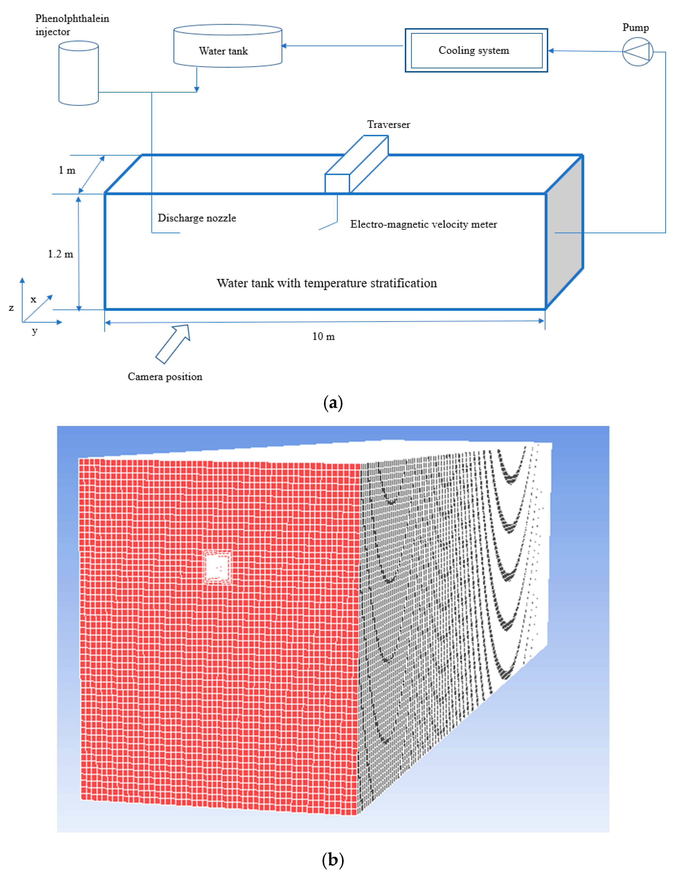
2.3. Model Description and Numerical Process

CFD simulations were performed using the commercial CFD code Fluent 17.2. The experimental configuration was implemented by the Gambit program, and the original model conditions were taken from the experimental data of Sakurazawa et al. and Fuji et al. [17,18]. Before the experiment started, the entire water tank was filled with temperature stratified water, the drainage time was set to 300 s, the time step was 0.1 s, and the maximum number of iterations for each time step was 20.

3. Analysis of Results

3.1. Cool Water Discharge

A numerical simulation is presented in which cold water was discharged into a temperature-stratified fluid. The simulation results were compared with previous research results.

Figure 2 shows the comparison results of previous experiments and the present numerical simulation. The solid line indicates previous experimental results, and the dashed line indicates the present numerical simulation results. The error range between previous experimental results and present numerical simulation results was 2.1~2.6%. In Figure 2, the v ratio is $v_r=v_2/v_1;$ the h ratio is $h_r=h-h_{in}/h$, where $h$ is the discharge inlet height, and $h_{in}$ is the intrusion depth of the discharge water in the tank.

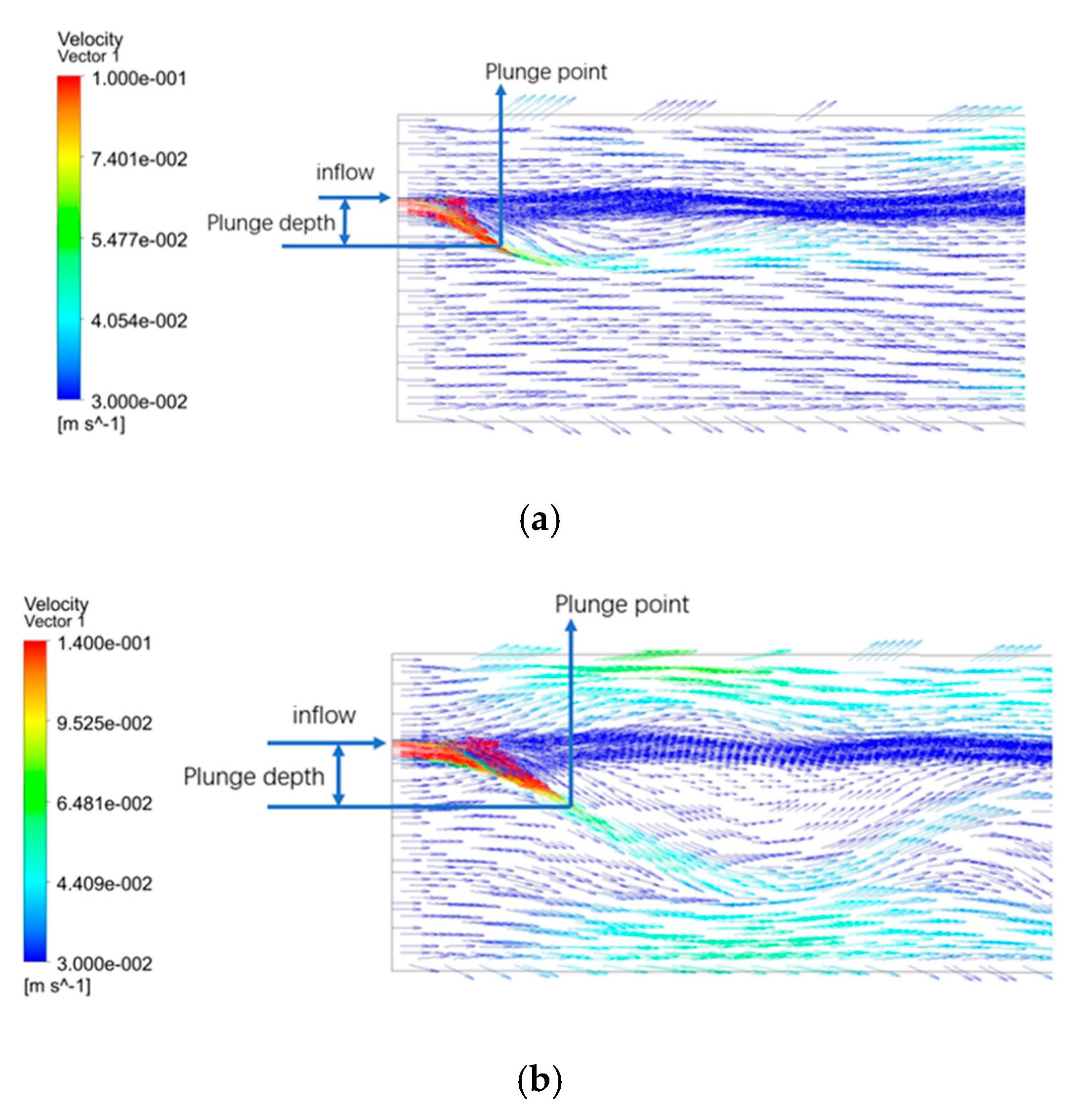
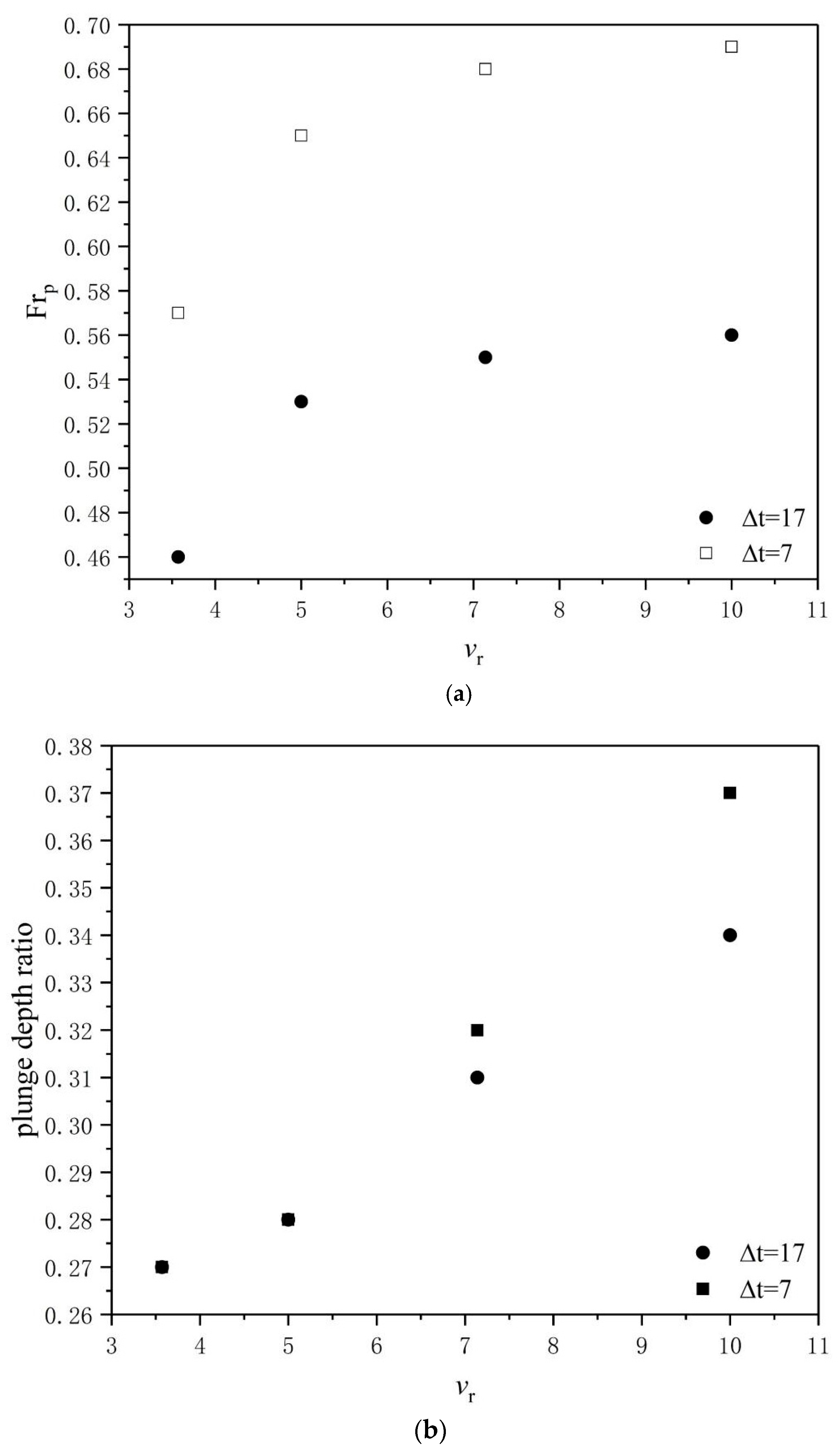
3.2. Plunging Phenomenon

The parameters of the plunging flow are obtained from the longitudinal center plane of the numerical model in the water channel, as shown in Figure 3. However, since the value of the plunging flow parameter is limited to the center plane, some errors are introduced. In the past, several researchers have proposed different standards for plunging flow models for their experiments based on dimensional analysis. For example, Singh and Shah [19] obtained the following equation (in centimeter units):

$$h_p=1.85+1.3{\left(\frac{q^2}{g^{\prime }}\right)}^{\raisebox{1ex}{$1$}\!\left/ \!\raisebox{-1ex}{$3$}\right.}$$

(10)

Farrell and Stefan [9] proposed the following general relationship:

$$h_p=k{\left(\frac{q^2}{g^{\prime }}\right)}^{\raisebox{1ex}{$1$}\!\left/ \!\raisebox{-1ex}{$3$}\right.}$$

(11)

where $h_p$ is the plunge depth; $k$ is a constant related to differences in concentration, temperature, and density; q is the discharge flow per unit width, and $g^{\prime }$ is the acceleration of gravity. Here $\mathrm{g}\prime =\mathrm{g}\Delta \mathsf{\rho }/{\mathsf{\rho }}_0$, where g is the acceleration of gravity. Also, $\Delta \rho =\rho -{\rho }_0$, where $\Delta \rho$ is the density difference between ambient water and inflow water, $\rho$ is the inflow water density, and ${\rho }_0$ is the ambient water density.

The definitions of the plunge depth and the plunge point were different from those used in previous studies. In this column, the plunge depth was the distance from the plunge point to the horizontal line of the discharge inlet. Therefore, how to determine the plunge point location was the primary problem that needed to be solved. The previous study mentioned that $q_0=v_0{h}_0=v_p{h}_p$, where the $h_0$ is the height of discharge inlet, for OTEC system, the $h_0$ would be replaced by the dimeter of cold water pipe; $v_p$ is the velocity of water at plunge point, means that the flow rate at the plunge point needs to be constant. Therefore, the plunge point position could be determined by numerical simulation, but there would be constraints, that is, the discharge water speed was faster than the ambient water speed, or the ambient water was in a relatively static state.

The plunge depths $h_p$ were plotted against ${\left(\frac{q^2}{g^{\prime }}\right)}^{\raisebox{1ex}{$1$}\!\left/ \!\raisebox{-1ex}{$3$}\right.}$, which was the parameter used by Singh and Shah [19] and Farrell and Stefan [9] to correlate their experimental data, as given in Figure 4. These results were fit to a line, and the coefficient k is expressed as an equation. [11] and that was extracted from the diagram for model simulation. Here, the k multiplier was 1.15. Singh and Shah [21] found that the k multiplier was 1.3, while Farrell and Stefan [9] found that the k multiplier was 1.6 based on the simulation results of 2D models. It can be seen from the results that the flow inlet conditions and the density difference between the flow inlet and the ambient water will affect the plunging position.

Figure 5 illustrates the flow characteristics of the discharge water. The plunging phenomenon was mainly affected by the difference in density and gravity. Figure 5a shows the specific location of the plunging point, where the horizontal axis shows the speed ratio between the velocity of discharge and the velocity of ambient water, and the vertical axis shows the densimetric Froude numbers. As the velocity of discharge water increased, the densimetric Froude numbers also became larger. As the temperature difference increased, the density difference also increased, which in turn led to a decrease in the densimetric Froude numbers. The densimetric Froude number can be written as follows:

$$F{r}_p=\frac{v_p}{\sqrt{g^{\prime }{h}_p}}$$

(12)

In the preceding equation, $g^{\prime }=g\frac{\rho -{\rho }_0}{{\rho }_0}$, $h_p$ is the plunging depth, $v_p$ is the velocity of the inflow at the plunging point, $\rho$ is the inflow fluid density, and ${\rho }_0$ is the ambient fluid density. The variation of the Froude number with the plunging depth is shown in Figure 5b. In Figure 5, the plunge depth ratio was $h_r=h_p/h$. According to Figure 5, the flow was subcritical because the Froude number at the plunge zone was less than 1 (Fr_p = 0.46~0.69). The minimum and maximum of the Froude number for different speed ratios are also shown in Figure 5a. The data obtained appear to be similar to those reported by Singh and Shah [19]. At the same speed ratio, the Froude number based on the lower temperature difference was greater than the one based on, the higher temperature difference. If the speed ratio is large enough ($v_r\ge 5$), the Froude number will not change significantly at the same temperature difference.

As understood from the results, the flow inlet condition and density influence the plunge location. The analysis of the plunging phenomenon of OTEC cold drainage on the ocean surface is of great significance for understanding the mixing and material transport of cold drainage and ocean surface water. The plunge point is the end of the streamflow and the starting point of the mixing phenomenon. According to the result analysis, the inflow densimetric Froude number would affect the plunging conditions. When the inflow densimetric Froude number is small, the distance that the inflow water sinks into the environment water body is short, but it should be pointed out that this short distance is difficult to distinguish by observation alone. The main reason is that the speed increase in the y-direction is relatively small in each case.

The results show that the numerical model used for density flow in reservoirs is applicable to the study of cold drainage in an OTEC system. This study examines only the plunging phenomenon of cold drainage in the OTEC system. It can be seen that the numerical simulation results are in good agreement with the experimental observations (shown in Figure 2). However, the limitations of this study are clear: the experiment cannot demonstrate the plunging point, and it is unknown whether plunging depth affects intrusion depth. Future work is needed to improve the numerical model with flow data obtained from real drainage of the OTEC system.

4. Conclusions

A 3D mathematical model is used to study the plunging phenomenon of inflow water in the water channel, and the relationship between the plunging parameters is also investigated. The effects of inflow conditions on the plunging phenomenon were discussed through model simulation. From the results, the model results are consistent with the experimental data, and the plunging depth is affected by changes in the ambient temperature difference. The Semi-empirical formula between the outlet flow and the plunging depth was obtained by model analysis, and the k multiplier was 1.15.

References

1. Bando, A.; Sakurazawa, S.; Umeki, M.; Ikegami, Y. Ocean Nutrient Enhancer “TAKUMI” for the experiment of Fishing Ground Creation. In Proceedings of the 3th IOES Symposium, Tsukuba, Japan, 5–19 September 2004; pp. 5–6. [Google Scholar]
2. Ouchi, K.; Otsuka, K.; Omura, H. Recent advances of ocean nutrient enhancer “TAKUMI” project. In Proceedings of the sixth ISOPE Ocean Mining Symposium, Changsha, Hunan, China, 9–13 September 2005; pp. 9–13. [Google Scholar]
3. Grandelli, P.; Rocheleau, G.; Hamrick, J.; Church, M.; Powell, B. Modeling the Physical and Biochemical Influence of Ocean Thermal Energy Conversion Plant Discharges into Their Adjacent Waters; U.S. Department of Energy Award NO. DE-EE0003638; Makai Ocean Engineering, Inc.: Kailua, HI, USA, 29 September 2012. [Google Scholar]
4. Akiyama, J.; Stefan, G.H. Plunging flow into a reservoir: Theory. J. Hydraul. Eng. 1984, 110, 484–499. [Google Scholar] [CrossRef]
5. Sequeiros, O.E. Estimating current turbidity conditions from channel morphology: A Froude number approach. J. Geophys. Res. Ocean. 2012, 117. [Google Scholar] [CrossRef]
6. Alavian, V. Behavior of density current on an incline. J. Hydraul. Eng. 1986, 112, 27–42. [Google Scholar] [CrossRef]
7. Alavian, V.; Jirka, G.H.; Denton, R.A.; Johnson, M.C.; Stefan, H.G. Density Currents Entering Lakes and Reservoirs. J. Hydraul. Eng. 1992, 118, 1464–1489. [Google Scholar] [CrossRef]
8. Dallimore, C.J.; Imberger, J.; Hodges, B.R. Modeling a plunging underflow. J. Hydraul. Eng. 2004, 130, 1068–1076. [Google Scholar] [CrossRef] [Green Version]
9. Poudeh, H.T.; Emamgholizadeh, S.; Fathi-Moghadam, M. Experimental study of the velocity of density currents in convergent and divergent channels. Int. J. Sediment Res. 2014, 29, 518–523. [Google Scholar] [CrossRef]
10. Farrell, G.J.; Stefan, H.G. Mathematical modeling of plunging reservoir flows. J. Hydraul. Res. 1988, 26, 525–537. [Google Scholar] [CrossRef]
11. Rodi, W. Example of calculation methods for flow and mixing in stratified fluids. J. Geophys. Res. 1987, 92, 5305–5328. [Google Scholar] [CrossRef]
12. Kassem, A.; Imran, J.; Khan, J.A. Three-dimensional modeling of negatively buoyant flow in diverging channels. J. Hydraul. Eng. 2003, 129, 936–947. [Google Scholar] [CrossRef]
13. Fukushima, Y.; Watanabe, M. Numerical simulation of density underflow by the k-ε turbulence model. J. Hydrosci. Hydr. Engrg. 1990, 8, 31–40. [Google Scholar] [CrossRef] [Green Version]
14. Ji, C.; Munjiza, A.; Avital, E.; Ma, J.; Williams, J. Direct numerical simulation of sediment entrainment in turbulent channel flow. Phys. Fluids 2013, 25, 056601. [Google Scholar] [CrossRef]
15. MacIntyre, S.; Sickman, J.; Goldthwait, S.; Kling, G. Physical pathways of nutrient supply in a small, ultraoligotrophic arctic lake during summer stratification. Limnol. Oceanogr. 2006, 51, 1107–1124. [Google Scholar] [CrossRef] [Green Version]
16. Hughes, G.O.; Griffiths, R.W. A simple convective model of the global overturning circulation, including effects of entrainment into sinking regions. Ocean Modell. 2006, 12, 46–79. [Google Scholar] [CrossRef]
17. Fuji, T.; Ikegami, Y.; Cai, W.X.; Monde, M. A Numerical Analysis of a Two-Dimensional Cool Water Jet into an Open Water Channel with Temperature Stratification. Bull. Soc. Sea Water Sci. Jpn. 2004, 58, 93–101. (In Japanese) [Google Scholar]
18. Sakurazawa, S.; Ikegami, Y.; Bando, A.; Umeki, M.; Monde, M. Influence of Thermal Stratification on the Penetration Depth of Cool Water Jet. Bull. Soc. Sea Water Sci. Jpn. 2005, 59, 292–300. (In Japanese) [Google Scholar]
19. Noto, K.; Matsushita, Y. Formulations and Direct Numerical Simulation Methods for Effects of Coriolis Forces, Latitude, and Stability Stratified Ambient on a Large-Scale Thermal Plume. Numer. Heat Transf. A 2007, 51, 363–392. [Google Scholar] [CrossRef]
20. Tatsumoto, H.; Park, J.; Machida, M.; Aikawa, M. Study on Behavior of Density Current in a Small Reservoir. J. Jpn. Soc. Hydrol. Water Resour. 2004, 17, 3–12. [Google Scholar] [CrossRef] [Green Version]
21. Singh, B.; Shah, C.R. Plunging phenomenon of density currents in reservoirs. La Houille Blanche 1971, 26, 59–64. [Google Scholar] [CrossRef] [Green Version]
Figure 1. Experimental schematic and numerical simulation grid diagram: (a) experimental setup [18] and (b) numerical simulation grid.
Jmse 08 00155 g001
Figure 2. Comparison of numerical simulation and experimental results: (a) comparison of depths and (b) intrusion depth of the discharge water in the tank [18].
Jmse 08 00155 g002
Figure 3. Typical tank velocity fields on a longitudinal cross-section: (a) v 2 / v 1 = 3.57 , ∆T = 17 and (b) v 2 / v 1 = 5 , ∆T = 17.
Jmse 08 00155 g003
Figure 4. Plunge depths from previous 2D studies and the present 3D model simulation results.
Jmse 08 00155 g004
Figure 5. Variation of plunge flow parameters: (a) densimetric Froude numbers and (b) plunge depth ratio.
Jmse 08 00155 g005