Residual Resistance of Displacement Vessels

Abstract

The hydrodynamics of the residual resistance of ships is formulated for the first time: the residual resistance of vessel displacement is the result of the formation of retaining bow waves, Kelvin wave systems and their interaction—as well as the action of viscosity, which is expressed in the form of a turbulent subsurface boundary layer. Michell’s integral is taken as a basis for calculations of residual resistance. The two corrections take into account the shear layer of wave surface and the shift of the Kelvin bow system by the retaining waves. The correlation of the calculated and experimental curves confirms the validity of the described hydrodynamics of residual resistance. This article is intended for specialists in the field of hydrodynamics of displacement vessels and for designers of the ship hull.

1. Introduction

The study presents a method for calculating the residual resistance to the theoretical line drawing of the displacement vessel. This problem is posed and solved for the first time in the history of this problem.

The problem of theoretical and calculated determinations of the resistance to the movement of a vessel has a long history, which is described in the article [1]. The need for an accurate calculation of the ship resistance to the theoretical drawing led to the fact that in 1963, a seminar on theoretical wave resistance was held in Ann Arbor (USA), at which a work plan was prepared for theorists, designers and experimenters in the field of shipbuilding of over the world. Over 13 years of intensive collaboration, hundreds of theoretical and experimental works in this field have appeared. In 1976, a seminar was organized in Tokyo to summarize the results. At this seminar, it was noted that despite the enormous efforts, the desired method for calculating the resistance of the vessel still was not formulated. The reasons for this failure is shown in the present article.

It should immediately be noted the main features of the problem of determining the resistance of ships.

The peculiarity of the situation with the definition of ship resistance is that we can now count with sufficient accuracy the frictional resistance created by the invisible boundary layer of the ship hull and a picture of the retaining and Kelvin waves is visible to the unaided eye, but we cannot calculate the resistance created by them.

(1)

The main feature of the problem of ship resistance is that it can be solved only by dividing the total resistance into components. Thus, the total resistance is equal to the sums

$$R=R_{\tau }+R_{\upsilon }+R_w=R_{\tau }+R_{res}$$

where $R_{\tau }$, $R_{\upsilon }$, $R_w$ and $R_{res}$ are the resistance of friction, vortex, wave and residual, respectively.

Unfortunately, calculation methods determine precisely only the frictional resistance, and the wave resistance only approximately by Michell’s integral [2].

(2)

It is important that these components of resistance do not depend on each other. The first proof of this independence was obtained from the experiments of G. Weinblum et al. [3] and S. Sharma [4] with long models;

The second experimental proof of this independence follows from the author’s experiment with the tandem of struts [5]. E. Baba gave the direct proof of this independence [6].

(3)

To date, the designer can obtain accurate information about the resistance of the particular ship hull using only model experiments. Residual resistance is obtained by the method of W. Froude, the viscous resistance is obtained by the Tulin–Betz method [7]; wave resistance can be experimentally obtained from “wave analysis” [8];

(4)

The calculated curve of the wave resistance according to Michell’s integral in its traditional form is obtained with humps and hollows (Figure 1), which do not exist on experimental curves; therefore, this Michell’s curve does not allow us to compare Michell’s curves of different models and estimate the wave resistance at a given speed. Our studies use a new form of Michell’s integral, which is devoid of the listed disadvantages [5];

If we take into account that not all experimental towing tanks are equipped with measuring instruments for obtaining viscous resistance by the Tulin–Betz method and for “wave analysis”, but all can now receive residual resistance, it is desirable to learn how to calculate the residual resistance. The article considers the solution to this problem.

The article contains four parts: (1) justification of the approach to solving this problem and a description of the calculation scheme; (2) study of the role of retaining waves and the way to take into account their action; (3) the subsurface boundary layer and its accounting; (4) results of calculations of the residual resistance of different models and ships. The main research results are given in the conclusion.

2. Basic Approaches to Solving the Problem of Residual Resistance

In order to understand the hydrodynamics of residual resistance, the basic conditions for solving this problem are formulated and the paradoxes that have arisen are considered.

The first condition—Engineering solutions are usually constructed when considering the first-order of the acting forces without taking into account their higher orders. For example, the solution of Michell constructed on the linearization of differential equation and boundary conditions gives the main part of the wave resistance and a better approximation to the experimental curves of the residual resistance than all higher order theories.

The second condition—Ship resistance is the result of the action of the hull of a moving ship on water, so it is necessary to look for sources of resistance components on the surface of the hull, rather than in a stream of waves and vortices outside it. The proof of this hypothesis is, for example, the Prandtl solution of the problem of frictional resistance. Michell also received his solution by integrating pressure over the surface of the hull.

The third condition—To identify the reasons for the discrepancy between the calculated curve of the wave resistance and the experimental one, it is necessary to find explanations for the paradoxes that arose in the process of solving this problem and, at the same time, remember the words of Leonardo da Vinci, that the experiment never deceives, our judgments deceive us.

The first paradox—In the calculations of water resistance of ships, the reversed motion of the vessel is usually considered, that is, the vessel is considered fixed, and the liquid is regarded as flowing to it at a constant velocity. This is true if the fluid is considered ideal, but in a real liquid, the Du Buat’s paradox must be taken into account.

The essence of Du Buat’s paradox is that the resistance of a body moving at a constant speed in a fluid at rest is greater than the resistance of the same, but motionless body, streamlined by the fluid at the same speed.

There are various explanations for this paradox, but in the case of vessel motion, the liquid is at rest, the body must overcome the inertial state of the viscous fluid at rest, which requires additional energy. When the fluid moves, the streamlines only slightly curve around the body, which requires little energy.

In any event, neglecting Du Buat’s paradox leads to the fact that in calculating water resistance the movement of ships under reversed motion does not take into account the formation of retaining waves associated with inertial properties of the fluid.

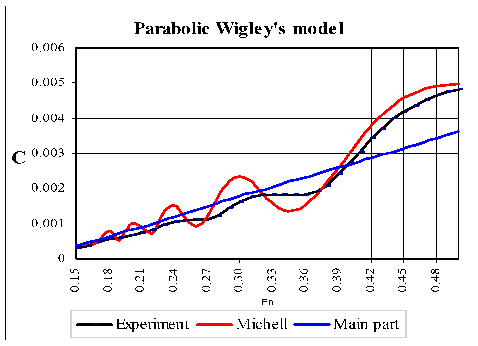
The second paradox—It is believed that the residual resistance is the sum of the wave and vortex resistance. Determining the wave resistance using Michell’s integral and comparing with the residual resistance from the experiment, we obtain the result for most of Weinblum’s and Wigley’s models, as shown in Figure 1, i.e., the curve of the residual resistance passes below the wave resistance curve. For comparison, a new form of Michell’s integral is used [5], described below in Equations (3)—(7).

This contradicts the physical meaning, because moving in an ideal fluid (as it is believed in Michell’s integral) is certainly easier than in a viscous fluid. This fact is a paradox.

The same comparison was made for different models to avoid accidents in such a mutual position of the calculated and experimental curves. The results are summarized in

Table 1. Comparison of the relative position of the main part of the calculated Michel’s curves and the experimental curves of the residual resistance (Wigley’s models).

No	Models	Angle of Entry α Grad	$\mathit{\beta }$	$\mathit{\delta }$	$\mathit{\phi }$	Fr = $0.15÷0.3$
1	Wg1846a	0.2913	0.666	0.498	0.747	Rw > Rres
2	WgN43	0.2366	0.909	0.799	0.879	Rw > Rres
3	Wg1846b	0.2226′	0.666	0.462	0.693	Rw > Rres
4	Parabolic	0.1978	0.556	0.444	0.667	Rw > Rres
5	Wg1970b	0.1978	0.667	0.467	0.700	Rw > Rres
6	Wg829	0.158	0.667	0.427	0.640	$Rw\le Rres$
7	Wg1970c	0.1003	0.671	0.467	0.700	Rw > Rees
8	Wg1805a	0.0748	0.666	0.391	0.587	Rw< Rres

and

Table 2. Comparison of the relative position of the main part of the calculated Michel’s curves and the experimental curves of the residual resistance (Weinblum’s models).

No	Models	Angle of Entry α Grad	$\mathit{\beta }$	$\mathit{\delta }$	$\mathit{\phi }$	Fr = $0.15÷0.3$
9	Wb1113	0.257	0.839	0.578	0.689	Rw > Rres
10	Wb1100	0.2366	0.839	0.579	0.690	Rw > Rres
11	Wb1097	0.2366	0.75	0.543	0.723	Rw > Rres
12	Wb1136	0.2366	0.929	0.619	0.666	Rw > Rres
13	Wb1110	0.2366	0.839	0.551	0.656	Rw = Rres
14	Wb1098	0.1375	0.75	0.520	0.692	Rw > Rres
15	Wb1114	0.1361	0.839	0.550	0.656	Rw = Rres
16	Wb1111	0.1075	0.839	0.542	0.647	Rw < Rres

. Michell’s curves were obtained with a correction taking into account the subsurface boundary layer of the ship’s waves. The rightmost column of Table 1 and Table 2 show the relative position of Michell’s curve R_w and the experimental curve of the residual resistance R_res in the range 0.15 < Fr < 0.3.

Table 1 and Table 2 show that, in addition to the entry angle $\alpha$ of the main waterline, the longitudinal fullness coefficient $\phi$ affects the mutual position of the calculated and experimental curves. The models in Table 1 are located in decreasing order of the entry angles $\alpha$ (the third column of tables). This is shown by the selection of those values $\phi =\delta /\beta$ ($\delta$-block coefficient, $\beta$-midship area coefficient) that explain the violation of order in the mutual position of the curves (in the sixth column).

The third paradox—In the famous experiment of G. Weinbum, J. Kendrick and M. Todd [3] with an elongated model, the calculated Michell’s curve coincides with the residual resistance curve (Figure 2) with all the humps and hollows at all Froude numbers. The authors of this experiment checked Michell’s first assumption that the width of the ship is considered small compared to its length. They made the model with L/B = 36, 7. However, Michell made his decision with three assumptions. He believed that the height of the ship waves is small in comparison with their length, and that the liquid is not viscous. For such a coincidence of the Michell’s curve with the residual resistance curve, the second and third assumptions must be satisfied, which means that the liquid behaved as ideal in this experiment. Why?

Another experiment, described in the author’s works [5,9,10] with a tandem of struts (Figure 3), causing two consecutive Kelvin systems of waves, can be added to Weinblum’s (Figure 2) experiment. It was assumed that the struts create, as sources, two Kelvin systems of waves. Although there is no ship hull with its boundary layer between the struts, the resistance curve of the tandem (Figure 4) had the same characteristics as the residual resistance curves of the displacement ship models, although it was assumed that the interaction of the two wave systems should give humps and hollows on the tandem resistance curve, as in Michell’s curve in Figure 1.

Then the second question arose: “Why does the fluid with the developed boundary layer in Weinblum’s [3] experiment behave as ideal—and in the case of thin struts with an aviation profile—in the absence of a hull of the ship with a boundary layer between them, there is an obvious influence of viscosity (in an ideal fluid curves would have humps and hollows)?” Both experiments prove that the boundary layer of the ship hull does not affect the wave resistance. However, this fact led to the thought of the role of the ship bow of the moving body in creating residual resistance. The entrance angle of the main waterline of the elongated model is approximately 2°, while the struts have an almost straight bow entry. Then the hypothesis of the existence of “impulse pressure” in the bow was formulated.

The waves created by the struts can be reduced only by turbulent viscosity, and only impulse pressure on the bow’s perpendicular could create turbulence flow. Hence, the turbulence flow is connected with the entrance angle of the active waterline. In Weinblum’s model [3], the angle of entry is so small that the impulse pressure is negligible, so that the effect of viscosity on the ship waves is small.

In order to accurately determine the hydrodynamics of the action of viscosity and its role in the residual resistance, it is necessary to understand what is happening at the stem of a moving vessel.

The accepted design scheme—Michell’s integral is the basis for calculating residual resistance for three reasons. First, this integral directly contains the derivatives of the waterlines of the theoretical drawing, reflecting in this way the exact shape of the ship hull instead of dimensions and parameters. Second, this integral accurately reflects the hydrodynamics of the ship’s wave system: the bow and stern Kelvin wave systems move away from the stem and the sternpost, and the derivatives of the waterline entering into Michell’s integral are also taken on the stem and the sternpost. Third, this integral is convenient for introducing corrections which take into account the effects of the subsurface shear layer and the shifting of the tops of ship waves by the retaining waves.

The new form of the Michell integral used in this work was obtained by integration over the length, which eliminated the errors of discretization of the ship hull surface length [5]. Thus, numerical integration is applied only at the last stage.

When a new form of the Michell integral is used, it is convenient to introduce corrections that take into account the effect of viscosity. In the new form of the Michell integral the main non-oscillating part is separated from the part responsible for interference of the fore and aft wave systems. In addition, contributions to the resistance from the fore and aft parts are also separated. Thus, the Michell integral with two corrections has the form:

$$R_w=\frac{4\rho g^2}{\pi {\upsilon }^2}{\left(\frac{B}{2}\right)}^2\cdot T^2\left[I_1^2+{(k_{turb}\cdot I_2)}^2\right],$$

(1)

where

$$I_1={\displaystyle \underset{0}{\overset{\pi /2}{\int }}{J}_4^2}\left(p\right)\cdot F_1\left(k\right)\frac{d\mathsf{\theta }}{{\cos }^3\mathsf{\theta }}$$

(2)

The equation of the hull surface for this calculation is presented in the form

$$y=b\cdot f_1(z)\cdot f_2(x)$$

(3)

$$I_2=2{\displaystyle \underset{0}{\overset{\pi /2}{\int }}{J}_4^2}\left(p\right)\left[F_2\left(k\right)cos2k+F_3\left(k\right)sin2k\right]\frac{d\mathsf{\theta }}{{cos}^3\mathsf{\theta }}$$

(4)

where

$$J_4(p)={\displaystyle \underset{0}{\overset{1}{\int }}{f}_1}\left(z\right)\cdot e^{-pz}dz$$

(5)

where

$$\begin{array}{l}{F}_1\left(1\right)=k^{-2}\left[G_{bo}^2+k^{-2}{G}_{b1}^2+G_{so}^2+k^{-2}{G}_{s1}^2\right];\\ F_2\left(1\right)=k^{-2}\left[G_{bo}{G}_{so}+k^{-2}{G}_{b1}{G}_{s1}\right];\\ F_3\left(1\right)=k^{-3}\left[G_{bo}{G}_{s1}-k^{-2}{G}_{b1}{G}_{so}\right],\end{array}$$

(6)

where $p=\frac{g}{{\upsilon }^2{\cos }^2\mathsf{\theta }},k=\frac{g}{{\upsilon }^2\cos \mathsf{\theta }}.$ Here $\mathsf{\theta }$—is the angle of integration. The indices $bo$ and $b1$ refer to the bow and the indices $so$ and $s1$ refer to the aft part of the hull.

Usually, all the derivatives entering into Formula (7) are taken in the Michell integral on the stem and at the sternpost at the points $x=1$ and $x=-1$, where indicated $g\left(1\right)=f_x^{\prime }\left(1,0\right)$, etc.

To account for the shift in the Michell integral, the shift correction in the form of a factor $k_{sd}$ is introduced to the function $g\left(1\right)$, which is the tangent of the entry angle $G_{bo}$ of the acting waterline (this is a function in Formula (7)).

$$\begin{array}{l}{G}_{b1}=g^{\prime }(1)-g^{‴}(1)k^{-2}+g^V(1)k^{-4}-\dots {(-1)}^{r+1}{g}^{(2r-1)}(1)k^{-(2r-2)},\\ G_{bo}=g(1)\cdot k_{sd}-g^{″}(1)k^{-2}+g^{IV}(1)k^{-4}\dots \{\begin{array}{l}{(-1)}^r{g}^{(2r-2)}(1)k^{-2r},ifm=2r+1,\\ {(-1)}^{r-1}{g}^{(2r)}(1)k^{-(2r-2)},ifm=2r,\end{array}\\ G_{s1}=g^{\prime }(-1)-g^{‴}(-1)k^{-2}+g^V(-1)k^{-4}-\dots {(-1)}^{r+1}{g}^{(2r-1)}(-1)k^{-(2r-2)},\\ G_{so}=g(-1)-g^{″}(-1)k^{-2}+g^{IV}(-1)k^{-4}\dots \{\begin{array}{l}{(-1)}^r{g}^{(2r-2)}(-1)k^{-2r},ifm=2r+1,\\ {(-1)}^{r-1}{g}^{(2r)}(-1)k^{-(2r-2)},ifm=2r.\end{array}\end{array}$$

(7)

The shift correction in (7) has the following form:

$$k_{sd}=k_1\pm k_2\cdot \left(Fr-F{r}_o\right)$$

(8)

where $Fr$ is Froude number, $F{r}_o$ is Froude number, from which the calculation begins. To account for the effect of the shear layer below the surface of ship waves, a correction $k_{turb}$ is introduced to the interference term of the Michell integral (1).

3. Retaining Waves and the Shift of the Bow Kelvin Wave System

The following information was known to us from Japanese works. E. Baba traced the path from the plane of the aft perpendicular, where he measured the loss of momentum, to the origin of the vortices at the place of breakdown of waves near the bow of ships [10]. According to our second condition, the source of the vortices should be sought on the surface of the hull, and not somewhere in the current, as E. Baba does. In the work of H. Miyata et al. [11] it is written: “It is intuitively understood that linear waves and nonlinear waves coexist around ships. Therefore, wave resistance of ships is supposed to be composed of two different wave systems. In other words, the flow field, where the Kelvin system begins, is covered by shockwaves on the free surface. Consequently, the interaction between the two wave systems will affect the resistance.” H. Miyata writes in all the following works on shock waves that the stern slope of shock waves has a turbulent nature and later H. Miyata and T. Inui write, “The displacement velocity by free surface is supposed to shift Kelvin pattern laterally”. This is shown in Figure 5 and Figure 6.

It should be noted that according to the known formula $rotgrad\phi =0$ from field theory, retaining waves and Kelvin waves cannot “coexist” in one space: Therefore, Miyata’s first statement is wrong, but the conclusion about the shift is true in these Japanese works. Notwithstanding, the fact of the shift of the bow Kelvin wave system by retaining bow waves is important because accounting for this shift, as will be shown later, leads to agreement the calculated resistance and the experimental results. Shift by retaining waves of the bow Kelvin wave system is clearly visible in photos of high-speed vessels in Figure 7a–d.

Shift correction—$k_{sd}=k_1\pm k_2\cdot \left(Fr-F{r}_o\right)$. It is easy to see that up to Fr = 0.4 there are the two Kelvin systems of waves. On the Froude number 0.4 only one transverse wave of the Kelvin system placed along the ship’s hull length and at higher Froude numbers the bow and stern systems of the waves are combined into one system, so there are no more humps and hollows on Michell’s curve as at small Froude numbers and the calculated Michell’s curve passes close to the experimental curve of residual resistance (Figure 1).

Consequently, the problem is to find a way to calculate the residual resistance of the vessel in the range of Froude numbers from 0.15 to 0.40.

Since the boundary layer of the ship hull has no effect on ship waves, the residual resistance is determined only by the retaining and ship waves and their interaction. Their interaction consists in a shift of the Kelvin wave system top by the retaining waves. This shift occurs on the ship hull surface, and therefore it must be taken into account of the resistance.

The main role of the shift correction is that it takes into account the effect of turbulent retaining waves on the Kelvin bow system. In this way, the first assumption of the smallness of the ratio of the width of the vessel to its length and the third assumption of Michell that the fluid is considered ideal is partially compensated.

The coincidence of the calculated curves obtained with the correction of the shift with the experimental curves for dozens of models proves that the calculation of the residual resistance based on the Michell integral with the correction of the shift correctly describes its nature (Figure 8). The interaction of the retaining and Kelvin waves can be taken into account as follows. The Michell integral (3) includes the first derivatives of the waterline on the fore and aft perpendiculars. Since the top of the bow wave system is shifted by the retaining waves to the stern direction, the derivative must be taken not at the fore perpendicular, but at the point in which this top is actually located. Despite the fact that Japanese scientists have noticed a shift of the Kelvin system, they have not taken it into account.

The meaning of the correction is visible in Figure 9. The following notation is accepted here: $\alpha$ angle of entry of main waterline, ${\alpha }_{sd}$—angle of the tangent line to the main waterline in the top of the Kelvin bow system. It is clear that for convex waterlines (Figure 9a), the shift leads to a decrease in the calculated entry angle (${\alpha }_{sd}<\alpha$) and for concave (Figure 9b)—to an increase. At very small entry angles, usually the waterline near the stem is concave, and the calculated Michell’s curve usually passes below the residual resistance curve. If we take the angle ${\alpha }_{sd}$ instead of the angle $\alpha$ on the stem, the calculated Michell’s curve will drop to the position of the residual resistance curve.

This fact explains the existence of the second paradox. The calculated Michell’s curve passes above the residual resistance curve because the actual angle of the tangent line to the main waterline at the position of the top of the bow Kelvin system is less than on the stem.

The relationship between the angles $\alpha$ and ${\alpha }_{sd}$ is much more complicated with a bend on the active waterline. If the waterline has any bend, the calculated Michell’s curve may pass above the experimental curve of the residual resistance, despite the small entry angle of the main waterline.

In order to take into account this shift, a correction is used in the form $k_{sd}=k_1\pm k_2\cdot \left(Fr-F{r}_o\right)$ It is impossible to find the general formula $k_{sd}=k_1\pm k_2\cdot \left(Fr-F{r}_o\right)$ for the correction of the shift, because it includes two coefficients $k_1$ and $k_2$, each of which depends on several parameters of the ship hull shape.

T. Inui said the same: “Owing to the high complexity of the bow-wave pattern, it is not possible yet to determine the amount of phase shift experimentally with the complicated hull” [12].

With sufficient accuracy for practice, it is possible to determine the correction of the shift only in the case when the waterline of the bow extremity has no bend; either straight or slightly convex.

Visual observation shows that the shape of the retaining waves depends on the speed of the vessel or its model. The sequence of stop-frames for the development of retaining waves with increasing velocity is shown in Figure 8. With increasing speed, the retaining waves are pressed increasingly to the surface of the body, which leads to a shift of the top of the bow Kelvin system of waves towards midsection.

For the study and calculations, the analytical models of G. Weinblum and W. Wigley are used, the data of which are given in Table 1, Table 2,

Table 3. Derivatives of the surface equations of the ship hull of Wigley’s models.

Models	${\mathit{k}}_{\mathit{s}\mathit{d}}={\mathit{k}}_1\pm {\mathit{k}}_2\cdot \left(\mathit{F}\mathit{r}-\mathit{F}{\mathit{r}}_{\mathit{o}}\right)$	f′(1)	f″(1)	f‴(1)	fIV(1)	fV(1)	fVI(1)	ao
Wg1805b	ksd = −0.0 − 4.0 × (Fr − 0.05)	0.00	0.08	2.40	2.40	0	0	0°00′
Wg1805a	ksd = 1.0 + 2.8 × (Fr − 0.15)	−0.08	0.40	14.40	1.44	0	0	4°17′
Wg1970c	ksd = 1.2 − 5.0 × (Fr − 0.16)	−0.10	1.35	10.65	42.13	94.50	94.50	5°45′
Wg829	ksd = 1.08 + 0.3 × (Fr − 0.15)	−0.16	0.00	0.48	0.48	0	0	8°00′
Wg1970b	ksd = 0.8 + 1.35 × (Fr − 0.15)	−0.20	0.15	3.15	13.65	31.65	31.65	11°20′
Пapaб.	ksd = 0.91 + 0.25 × (Fr − 0.15)	−0.20	−0.20	0	0	0	0	11°20′
Wg1846b	ksd = 0.7 + 2.0 × (Fr − 0.16)	−0.24	−0.40	−0.48	−0.48	0	0	12°42
Wg1846a	ksd = 0.0.45 + 4.1 × (Fr − 0.15)	−0.32	−0.08	−1.44	−1.44	0	0	16°41′

,

Table 4. Derivatives of the surface equations of the ship hull of Weinblum’s models.

Models	${\mathit{k}}_{\mathit{s}\mathit{d}}={\mathit{k}}_1\pm {\mathit{k}}_2\cdot \left(\mathit{F}\mathit{r}-\mathit{F}{\mathit{r}}_{\mathit{o}}\right)$	f′(1)	f″(1)	f‴(1)	fIV(1)	fV(1)	fVI(1)	ao
Wb1111	ksd = 1.3 − 4.5 × (Fr − 0.15)	−0.11	1.43	11.6	46.6	105.1	105.12	6°10′
Wb1114	ksd = 1.0 + 0.001 × (Fr − 0.15)	−0.14	0.36	2.2	−0.97	−55.6	−286.1	7°48′
Wb1098	ksd = 0.67 + 1.0 × (Fr − 0.16)	−0.14	0.6	5.1	18.0	34.8	28.80	7°56′
Wb1136	ksd = 0.0.8 + 0.65 × (Fr − 0.15)	−0.24	−0.08	2.4	12.0	28.8	28.80	13°31′
Wb1100	ksd = 0.8 + 0.8 × (Fr − 0.15)	−0.24	−0.08	2.4	12.0	28.8	28.80	13°31′
Wb1110	ksd = 1.0 + 0.01 × (Fr − 0.15)	−0.24	−0.08	2.4	12.0	28.8	28.80	13°31′
Wb1097	ksd = 0.8 + 0.3 × (Fr − 0.15)	−0.24	−0.08	2.4	12.0	28.8	28.60	13°31′
Wb1113	ksd = 0.82 + 0.1 × (Fr − 0.15)	−0.24	0.31	5.9	27.4	64.4	64.44	14°39′

and

Table 5. Data on the models of Wigley and Weinblum Wigley’s model: L = 4.876m, B =0.457 m, T = 0.3048 m, $L/B$ = 10.67, $L/B$ = 1.5. Weinblum’s model: L = 4.5m, B = 0.45 m, T = 0.18 m, $L/B$ = 10, $L/B$ = 2.5.

No	Wigley’s and Weinblum’s Models	Angle of Entry of Waterline	$$\mathit{\beta }$$	$$\mathit{\delta }$$	$$\mathit{\phi }$$	$${\mathit{k}}_1$$	$${\mathit{k}}_2$$	$${\mathit{v}}_{\mathit{t}\mathit{u}\mathit{r}\mathit{b}}$$
1	Wg1805b	0°00′	0.666	0.355	0.533	0.0	−4.0	0.08
2	Wg1805a	4°17′	0.666	0.391	0.587	1.0	2.8	0.05
3	Wg1970c	5°45′	0.671	0.467	0.700	1.2	−5.0	0.08
4	Wb1111	6°10′	0.839	0.542	0.647	1.30	−4.5	0.05
5	Wb1114	7°48′	0.839	0.550	0.6565	1.0	−0.001	0.08
6	Wb1098	7°56′	0.75	0.519	0.693	0.67	0.1	0.08
7	Wg829	8°00′	0.656	0.427	0.640	1.08	0.3	0.08
8	Wg1970b	11°20′	0.671	0.467	0.700	0.8	1.35	0.08
9	Parabolic	11°20′	0.666	0.444	0.667	0.91	0.25	0.08
10	Wg1846b	12°42′	0.666	0.355	0.693	0.7	2.0	0.08
11	Wb1100	13°31′	0.839	0.579	0.69	0.8	0.8	0.08
12	Wb1110	13°31′	0.839	0.550	0.656	1.0	0.01	0.08
13	Wb1097	13°31′	0.75	0.519	0.693	0.8	0.3	0.08
14	Wb1136	13°31′	0.929	0.619	0.666	0.8	0.65	0.08
15	Wb1113	14°39′	0.839	0.578	0.69	0.82	0.1	0.08
16	Wg1846a	17°41′	0.666	0.391	0.587	0.45	4.1	0.08

. The models taken for the calculation had different shapes of the main waterlines, as shown in Figure 10 and Figure 11. The choice of these models is justified by the fact that we have the G. Weinblum and W. Wigley experiments of fairly accurate. The calculation results are given in Section 4 (Table 7).

It is clear from this study that the coefficient $k_1$ in (8) takes into account the change in the angle of entry ${\alpha }_{sd}$ at the main waterline at the beginning of the movement. The coefficient $k_2$ takes into account the dependence of the shift of the top of the bow Kelvin system on the speed of the vessel or model. Even such a simple study, which is shown in Table 3, Table 4 and Table 5, shows that the coefficients $k_1$ and $k_2$ are very complex depending on the hull.

It must be taken into account that shift correction, how it is used in this work, takes into account not only the shift of the Kelvin wave system, but also a decrease in pressure in the stern of the ship’s hull.

Comment. In order to determine the correction $k_{sd}=k_1\pm k_2\cdot \left(Fr-F{r}_o\right)$ empirically, it is necessary to divide the hull shapes of different ships into types and experimentally obtain for each type the coefficients values $k_1$ and $k_2$ depending on hull parameters.

When there are waves on the flow of fluid, a velocity gradient naturally is formed below the free surface. A typical experimentally picture of the velocity distribution under the free surface of a wave near the moving ship model is shown in Figure 12. The gradient of velocity is called the “shear layer.” The destruction of waves is associated with the existence of this shear layer. Studies of the shear layer began intensively after E. Baba [10] took note of the flow of vortices creating a loss of momentum in the plane of the aft perpendicular. In 1970, S. Taneda [13] E. Eckert and S. Sharma [14] were engaged in experimental study of vortices around the bow of the vessel. The article by K. Taniguchi et al. [15] on the investigation of the wake was published a year later. K. Takekuma published the article [16] on nonlinear waves around the ship bow next year and a year later an article by E. Eckert and S. Sharma [14] on the bulbous form of the bow, which appeared to suppress the bow wave creating the vortex was published.

In the late eighties and early nineties, the results of experimental studies of the shear layer under a free wave surface were published by V. Melvil with V. Rapp [17], J. Duncan et al. [18], J. Lin and D. Rokwell [19]. It is necessary to note the work done in the basin of David Taylor (USA) R. Dong, J. Katz and H. Huang [20]. The studies were carried out using a PIV speedometer with the image of the fluid particles in the flow around the ship model, with attention focused on the flow inside the liquid layer, upward from which the bow waves separate from the surface of the model. In addition, the origin and structure of the bow wave and the stream downstream from the crest of the wave were studied.

In addition to the experimental works and theories were developed methods for calculating resistances associated with a shear layer under a free wave surface around a moving vessel. Naturally, they give good reviews. Here we should mention the survey works of D. H. Peregrine, L. A. Svendsen [21] in 1978 and M. Banner with D. Peregrin [22] in 1993. Good analytical reviews were performed by L. Rahedzia [23], [24] in 1986 and then in 1995.

Theoretical approaches to turbulence were developed by G. Dagan and M. Tulin [25], J. Vanden-Brock and E. Tuck [26], H. Miyata and T. Inui [27], E. Baba and K. Takekuma [28], G. Vanden-Brock, M. Shvarts and E. Tak [29], K. Eggers [30], T. Inui [11], K. Mori [31], A. Shahshahan [32], J. Hoyt and R. Sellyn [33], M. Longe-Higgins and E. Kokelet [34], R. Cointe and M. Tulin [35], E. Pogozelsky, J. Katz, T. Huang [36].

As a result of the studies performed, it was concluded that:

(1)

The shear layer on the free surface and the vortices in it are closely related to the destruction of waves around the bow;

(2)

A draft in the bow, an extended underwater bulb, the angle of the bow entrance and the contours of the waterline greatly affect the shear under the free surface and the vortices in it;

(3)

With the exception of a thin layer below the free surface, the velocity components obtained by measurements coincided with the results of numerical calculations based on the assumption of a double model;

(4)

The velocity components change sharply in this thin layer in the vertical direction (Figure 12);

(5)

The shear layer of the ship’s wave system affects only the interaction of the bow and stern of the Kelvin wave systems, because this shear layer is outside the ship’s hull and cannot act on the part of the resistance, determined by the main part of Michell’s integral.

$$\eta =\frac{1}{2}\sqrt{\frac{g}{\pi }}\frac{St}{x^{3/2}}\exp \left(-vgt/g^3\right)\cos \left(\frac{g{t}^2}{4x}-\frac{\pi }{4}\right)$$

(9)

Correction$k_{turb}$. In order to obtain a coefficient that takes into account the viscosity of the subsurface shear layer, Sretensky’s formula for calculating the wave height in the Cauchy-Poisson problem for a viscous liquid is used [4]:

If we assume that the time $t$ is equal to the time for which the bow waves reach the point of wave formation in the stern, then, by substituting $t$ into Sretensky’s formula, this correction is obtained in the form:

$$\exp (-\nu /L^{3/2}/g^{1/2}/F{n}^5)$$

Since the coefficient of molecular viscosity $v$ practically has no effect on the height of the water wave, it is necessary to replace it with the coefficient of turbulent viscosity $v_{turb}$. Then it raises the question of the possibility of a simple replacement of the coefficient of molecular viscosity $v$ by the coefficient of turbulent viscosity $v_{turb}$. Since such a substitution was made in the diffusion problem by N.E. Kochin, we considered it possible to make the same substitution in this case. The next problem is the exact determination of the coefficient $k_{turb}$. In our case, this coefficient has the form

$$k_{turb}=\exp (-{\nu }_{turb}/L^{1/2}/g^{1/2}/F{n}^5)$$

(10)

here ${\nu }_{turb}$ is half the coefficient of turbulent viscosity. Unfortunately, this coefficient $k_{turb}$ depends on the dimensional value L. Since Michell’s integral in our case gives the coefficient of wave resistance and not the resistance itself, one can always take into account the length would have a value 4.5–5.0 m and $v_{turb}$ should be in the range 0.05 ÷ 0.08. This is evident from Table 5.

Regarding the correction $k_{turb}$, taking into account the subsurface boundary layer of Kelvin waves, the following should be noted. Judging by the formation of a necklace of vortices, this boundary layer has a turbulent nature and it would have to be calculated using RANS. But to use RANS in this case, special studies are still needed, perhaps more complicated than to obtain an correction, therefore, in this case, approximate values are accepted, especially because this correction varies in a small range.

Among Weinblum’s models, there are 4 models Wb1110 Wb1100, Wb1136, Wb1097 having the same dimensions and the entrance angle, but the experimental residual resistance curves and main part of Michell integral turned out as different (

Table 6. Comparison of the hull ship parameters of the models with $\alpha =0.2356$.

Models	$$\mathit{\beta }$$	$$\mathit{\delta }$$	$$\mathit{\phi }$$	$${\mathit{k}}_1$$	$${\mathit{k}}_2$$
Wb1110	0.839	0.551	0.656	1.0	0.2
Wb1136	0.929	0.619	0.673	0.8	0.7
Wb1100	0.839	0.579	0.690	0.7	1.5
Wb 1097	0.750	0.543	0.723	0.6	1.6

).

Of course, it is natural to analyze the influence of the shape parameters on the resistance using these models. The graph (Figure 13) clearly shows the relationship between the coefficient of longitudinal fullness $\phi$ and the relative position of the experimental curves of the residual resistance.

The Wb1110 has the smallest coefficient $\phi$ and the resistance curve passes below the others. The Wb1100 model has the largest coefficient $\phi$ and the residual resistance curve passes above the others. It turns out that to reduce the resistance, it is necessary to reduce the coefficient of longitudinal fullness $\phi =\delta /\beta$ as much as possible, which in general does no contradict common sense. To reduce this coefficient, it is possible by increasing the fullness of the coefficient $\beta$; shifting the displacement to the midsection.

The same conclusion was obtained by decreasing the wave resistance using the Michell integral [5].

In order to obtain the general calculated formula special empirical and experimental studies are required. It is necessary to find the dependence of turbulence, i.e., coefficients $v_{turb}$ and $k_{turb}$ on the shape parameters of the hull. In this study, they are assumed to be constant, but turbulence cannot be independent on the speed of the vessel. Judging by the numerous calculations for different models, this dependence is very small.

4. Results of Residual Resistance Calculations

Calculations were performed for series of analytical models of W. Wigley and G. Weinblum. The results of the residual resistance calculations are summarized in

Table 7. Examples of calculations of residual resistance G.Weinblum and W.Wigley models.

The curve of the coefficient of the experimental curve of the residual resistance (black) and the Michell curve (pink) and its main part (blue)	Comparison of the experimental (black) and calculated curves of the residual resistance (red) with the correction.

. The left column shows the experimental curve of the residual resistance, the Michell curve and its main part (by (4)). The calculated Michell’s integral with all corrections and experimental residual resistance curves are shown in the right column. The waterlines of these models are shown in Figure 10 and Figure 11.

Calculations were also performed for four models the river ships “Rodina” and “Sevan” (

Table 8. Experiments and calculations wave and residual resistance of the river ships “Rodina” and “Sevan”.

The curves of the coefficient of the experimental curve of the residual resistance (black) and the Michell curve (pink) and its main part(blue)	Calculation of the residual resistance of models taking into account the shift by retaining waves of the bow waves system. Correction of the main part of Michell’s integral (blue line)

) and for five Todd’s models [37], [38] of series 60 (

Table 9. Calculation of residual resistance of the Todd model series.

Comparison of Michell’s integral (pink curve) and its main part (blue curve) with experimental residual resistance (black curve) of Todd models.	Calculation of the residual resistance of Todd’s models taking into account the shift by retaining waves of the bow waves system. Correction of the main part of Michell’s integral (blue line).

). All of this models cover a wide range of hull forms for displacement ships (Figure 10, Figure 11 and Figure 14).

For this calculation of Michell’s integral of the real ship, the hull surfaces are given in the form of an analytical grid, the description of which is given in papers [9,39]. En example of the accuracy of such approximation is shown in Figure 15.

Japanese researchers based the calculations of vortex resistance (not residual) on position: “Ships in translational motion generate a kind of shock wave as well as linear dispersive waves and the former has pertinent characteristics to be named as “free surface shock wave”. They use the theory of shock waves and the theory of motion in shallow water to calculate the resistance. In this case they get the approximation shown in Figure 16.

5. Conclusions

(1)

In this work, the hydrodynamics of residual resistance of the vessel is studied;

(2)

Shown, that the residual resistance is a result of the formation of retaining bow waves, Kelvin wave systems and their interaction, as well as the action of viscosity in the form of a turbulent subsurface boundary layer;

(3)

To test the new hydrodynamic theory of residual resistance a scheme for its calculating based on the Michell’s integral was developed;

(4)

Numerous calculations for different ship models confirmed the validity of a new understanding of the hydrodynamics of residual resistance;

(5)

The excellent coincidence of the calculated residual resistance curves with experiments for dozens of models proves that the hydrodynamic nature of the residual resistance is correctly understood;

(6)

The most important thing is here in the possibility of comparing the calculation of the residual resistance with the results of towing tests using the Froude method. This approach is simpler than the Tulin–Betz method of determining the viscous resistance and is also simpler and more accurate than any kind of “wave analysis”(See calculation in Table 7, Table 8 and Table 9);

(7)

The possibility of calculating the residual resistance using the theoretical drawing would solve the problem of optimizing the ship hull and the propulsion of the displacement vessel in the design process;

(8)

The disadvantage of this study is that all coefficients entered into the calculation formula were chosen empirically. However, the fact that they can be selected until the calculated curve coincides with the experimental residual resistance curve allows us to hope that the dependence of each of these coefficients on the shape parameters can be found experimentally;

(9)

From the foregoing it is clear that the researchers of 1963–1976 were doomed to failure because all calculation performed with reverse movement, that is, Du Buat’s paradox and the action the retaining waves were not taken into account.

To solve the problem of determining the residual resistance theoretically, it is necessary to develop a theory of interaction of the hyperbolic and elliptic flow with a free surface—if at all possible to do. The description of the existence of these fields around a moving ship is in a single work—in Eggers’s study on the dispersive waves of a flow around a moving vessel [30], where Figure 17 clearly shows the regions of the hyperbolic and elliptic flow.

Comment. The important question is about the possibility of using the scheme given in this study by designers. It is clear from the given examples that in the small and medium Froude numbers it is possible to estimate the resistance using the main part of Michell’s integral without introducing corrections (left part of Table 5 and Table 6). This is confirmed for real river vessels “Rodina” and “Sevan”, as well as for Todd’s models.

References

1. Gotman, A.S. A History of Ship Resistance Evaluation. J. Ocean. Technol. 2007, 2, 74–96. [Google Scholar]
2. Michell, J.H. The wave resistance of a ship. Philos. Mag. 1898, 45, 106–123. [Google Scholar] [CrossRef]
3. Weinblum, G.P. Investigation of Wave Effects Produced by a Thin Body—TMB Model 4125; Report 840; Navy Department, the David W. Taylor Model Basin: Washington, DC, USA, 1952. [Google Scholar]
4. Sharma, S.D. Some results concerning the wavemaking of a thin ship. J. Ship Res. 1969, 13, 72–81. [Google Scholar]
5. Gotman, A.S. Study of Michell’s integral and influence of viscosity and ship hull form on wave resistance. Ocean. Eng. Int. 2002, 46, 74–115. [Google Scholar]
6. Baba, E. Study on separation of ship resistance components. J. Soc. Nav. Arch. Jpn. 1969, 1969, 9–22. [Google Scholar] [CrossRef]
7. Tulin, M.P. The Separation of Viscous Drag and Wave Drag by Means of the Wake Survey; Report 772; Navy Department the David W. Taylor Model Basin DTMB: Washington, DC, USA, 1951. [Google Scholar]
8. Eggers, K.W.H. Wave Analysis State of the Art 1975 Intern. In Seminar on Theor; Wave Resistance: Tokyo, Japan, 1976; pp. 93–103. [Google Scholar]
9. Gotman, A.S. Theoretical and Experimental Bases of Hydrodynamics of Displacement Vessels Novosibirsk State Technical University. 2018. 615p. Available online: http://www.shipdesign.ru/Gotman (accessed on 27 March 2020). (In Russian).
10. Baba, E. A new component of viscous resistance of ships. J. Soc. Nav. Arch. Jpn. 1969, 125, 23–34. [Google Scholar] [CrossRef] [Green Version]
11. Miyata, H. Free Surface Shock Waves around Ships and Their Effects on Ship Resistance. J. Soc. Nav. Arch. Jpn. 1980, 147, 1–9. [Google Scholar] [CrossRef]
12. Inui, T. From Bulbous Bow to Free-Surface Shock Wave—Trends of 20 Years’ Research on Ship Waves at the Tokyo University Tank. J. Ship Res. 1981, 25, 147–180. [Google Scholar]
13. Taneda, S.; Amamoto, H. Necklace Vortex around Bow Bulletin of the Research Institute on Applied Mechanics; Kyushu University: Fukuoka, Japan, 1969; p. 31. [Google Scholar]
14. Eckert, E.; Sharma, S.D. Bugwijlste for Iangsame vollige Schiffe. Jahrb. Schiffbautech. Gesselschaft 1970, 4, 129–171. (In German) [Google Scholar]
15. Tanigachi, K.; Tamura, K.; Baba, E. Reduction of Wave-Breaking Resistance; Mitsubishi Heavy Industries Limited: Tokyo, Japan, 1972; pp. 62–69. [Google Scholar]
16. Takekuma, K. Study on Non-Linear Free Surface Problem around Bow. J. Soc. Nav. Arch. Jpn. 1972, 132, 1–9. [Google Scholar] [CrossRef]
17. Melville, W.K.; Rapp, W.M. The surface velocity field in steep and breaking waves. J. Fluid Mech. 1988, 189, 1–22. [Google Scholar] [CrossRef] [Green Version]
18. Duncan, J.H. The formation of spilling breaking water waves. Phys Fluids 1994, 6, 2558–2560. [Google Scholar] [CrossRef]
19. Lin, J.C.; Rockwell, D. Instantaneous of spilling breakers. Phys. Fluids 1994, 6, 2877–2879. [Google Scholar] [CrossRef]
20. Dong, R.R. On the structure of bow waves on a ship model. J. Fluid Mech. 1997, 346, 77–115. [Google Scholar] [CrossRef]
21. Peregrine, D.H.; Svendsen, L.A. Spilling Breakers bores and hydraulic jumps. In Proceedings of the 16th International Conference on Coustal Engingeer, Hamburg, Germany, 27 August–1 September 1978; Volume 1, pp. 540–550. [Google Scholar]
22. Banner, M.L.; Peregrin, D.H. Wave breaking in deep water. Ann. Rev. Fluid Mech. 1993, 25, 373–397. [Google Scholar] [CrossRef]
23. Raheja, L.R. Free Surface Shear Flow Model for Bow Vortices Phenomena; Hamburg Technische Universität: Hamburg, Germany, 1986. [Google Scholar]
24. Raheja, L.R. Free Surface Boundary Layer Approach to Study Bow Vortices Generation Ahead of a Semisubmerged Horizontal Circular. J. Ship Res. 1995, 39, 284–296. [Google Scholar]
25. Dagan, G.; Tulin, M. Two-dimensional free-surface gravity flow past blunt bodies. J. Fluid Mech. 1972, 51, 529–543. [Google Scholar] [CrossRef]
26. Vanden-Broeck, J.-M.; Tuck, E.O. Computation of near-bow or stern flows using series expansion on the Froude number. In Proceedings of the Second International. Conference on Numerical Ship Hydrodynamics, Berkeley, CA, USA, 19–21 September 1977; pp. 377–387. [Google Scholar]
27. Miyata, H.; Inui, T. Nonlinear ship waves. Adv. Appl. Mech. 1984, 24, 215–288. [Google Scholar]
28. Baba, E.; Takekuma, K. A study on free-surface flow of slowly moving full forms. J. Soc. Nav. Arch. Jpn. 1975, 137, 1–10. [Google Scholar]
29. Vanden-Broeck, J.-M. Divergent low Froude-Number series expansion of nonlinear free-surface flow Problems. Proc. R. Soc. Lond. Ser. A. 1978, 361, 207–224. [Google Scholar]
30. Eggers, K. Non-Kelvin Dispersive Waves around Non-Slender Ships. Schiffstechnik 1981, 28, 223–251. [Google Scholar]
31. Mori, K. Necklace Vortex and Bow Wave Around Blunt Bodies. In Proceedings of the 15th ONR Symposium on Naval Hydrodynamics, Humburg, Germany, 2–7 September 1984. [Google Scholar]
32. Shahshahan, A. A Study of a Free Surface Flow Near a Ship Bow. Master’s Thesis, Institution of Hydraulic Research, The University of Iowa, Iowa City, IA, USA, 1981. [Google Scholar]
33. Hoyt, J.; Sellin, R.H.T. The hydraulic jump as a mixing layer. Div. ASCE 1989, 151, 1607–1614. [Google Scholar] [CrossRef]
34. Longuet-Higgins, M.S.; Cokelet, E.D. The deformation of steep surface waves on water. I. A. Numerical method of computation. Proc. R. Soc. Lond. A 1976, 350, 1–26. [Google Scholar]
35. Cointe, R.; Tulin, M. A theory of spilling breaker. J. Fluid Mech 1994, 276, 1–20. [Google Scholar] [CrossRef]
36. Pogozelski, E.M. The foow structure around a surface piercing strut. Phis. Fluids 1996, 9, 1387–1399. [Google Scholar] [CrossRef]
37. Bai, K.J. Overview of results Proc. Workshop Ship Wave-resistance Computations; David W. Taylor Naval Ship Research and Development Center: Bethesda, MD, USA, 1979; Volume 1, pp. 33–37. [Google Scholar]
38. Todd, F.H. Series Methodical Experiments with Models of Single-Screw Merchant Ships; Report 1712; Maritime Technical Information Facility: Washington, DC, USA, 1963. [Google Scholar]
39. Gotman, A.S.; Krasnov, A.V.; Krasnov, A.V. Calculating of resistance of displacement ships of arbitrary hull form using the analytical grid. Proc. X Intern. Conf. Hydrod. 2012, 1, 160–165. [Google Scholar]
Figure 1. Calculated Michell’s curve (red) and its main part (blue) passes above the residual resistance curve (black)
Jmse 08 00400 g001
Figure 2. Testing of the long model. L/B = 36, 7. Points show the calculated results.
Jmse 08 00400 g002
Figure 3. Wave formation during movement of tandem struts (on the left—forward motion with a blunt end on the right—with a sharp end, L = 0.914 m, upper Fr = 0.161, lower Fr = 0.356).
Jmse 08 00400 g003
Figure 4. Experiment with the tandem struts. Fn is determined by the distance between the bow perpendiculars of the struts; the lower curve—R residual resistance of one strut, the upper curve—R of the twice the resistance of one strut; the red curve—R of the tandem of struts. The forward motion with a blunt end.
Jmse 08 00400 g004
Figure 5. Contours of waves, wave height in mm. In the bow you can see how the retaining waves shift the Kelvin wave system Fn = 0.267. The inscription at the top: “measured and koL = 14”; on the contour—”M42 and L = 20 (m)”.
Jmse 08 00400 g005
Figure 6. Contours of waves in the near model (wave height in mm) Fn = 0.267.
Jmse 08 00400 g006
Figure 7. Photos of ships with the visible shift of the bow Kelvin waves system. (a) Yacht of the English shipyard Sunseeker; (b) American aircraft carrier; (c) destroyer; (d) cruiser of the project 1164type “Atlant”.
Jmse 08 00400 g007
Figure 8. Dependence of the shape of the retaining waves on the speed of motion of the model. (a) Velocity 0.842 m/s (Fr = 0.161); (b) velocity 0.945 m/s (Fr = 0.180); (c) velocity 1.059 m/s (Fr = 0.202); (d) velocity 1.162 m/s (Fr = 0.222); (e) velocity 1.272 m/s (Fr = 0.242); (f) velocity 1.390 m/s (Fr = 0.265); (g) velocity 1.634 m/s (Fr = 0.312); (h) velocity 1.849 m/s (Fr = 0.353); (i) velocity 1.982 m/s (Fr = 0.378)
Jmse 08 00400 g008aJmse 08 00400 g008b
Figure 9. To the shift of the top of the Kelvin wave system. α : angle of entry of main waterline, α s d : angle of the tangent line to the main waterline in the top of the Kelvin bow system.
Jmse 08 00400 g009
Figure 10. Main waterlines of Weinblum’s models.
Jmse 08 00400 g010
Figure 11. Main waterlines of Wigley’s models.
Jmse 08 00400 g011
Figure 12. Example of the distribution of velocity components on a vertical plane parallel to the diametrical plane of wedge-shaped model [10].
Jmse 08 00400 g012
Figure 13. Weinblum’s models with the same dimensions and entry angle of the main waterline. (a) Residual resistance; (b) main part of Michell integral of these models.
Jmse 08 00400 g013
Figure 14. Main waterlines of Todd’s models of series 60.
Jmse 08 00400 g014
Figure 15. Comparison of (a) real and (b) calculated cross sections of Todd’s model. Points show calculated values.
Jmse 08 00400 g015
Figure 16. Comparison of wave pattern resistance of WM1 (This is Figure 16 in [23]).
Jmse 08 00400 g016
Figure 17. “Hyperbolic” and “elliptic” domains in the flow around the moving ship [30].
Jmse 08 00400 g017