Modeling of Autonomous Underwater Vehicles with Multi-Propellers Based on Maximum Likelihood Method

Abstract

The hydrodynamic characteristics of multi-propeller autonomous underwater vehicles (AUV) is usually complicated and it is difficult to obtain an accurate mathematical model. A modeling method based on CFD calculation and maximum likelihood identification algorithm is proposed for this problem. Firstly, rough hydrodynamic parameters of AUV hull are obtained by CFD calculation. Secondly, on the basis of rough parameters, a maximum likelihood identification algorithm is proposed to adjust the parameters and improve the model precision. Besides, the method to improve the convergence of identification algorithm is analyzed by considering the characteristics of AUV model structure. Finally, the identification algorithm and identification results were validated with experimental data. It was found that this method has good convergence and adaptability. In particular, the identification results of turning force and torque parameters are highly consistent in different identification experiments, which indicates that this method can well extract the maneuvering characteristics of AUVs, thus contributing to the controller design of AUVs. The research of this paper has potential application for the modeling and control of multi-propeller AUVs.

1. Introduction

Autonomous underwater vehicles (AUV) are used to perform a variety of tasks, including marine research, hydrologic survey, environmental monitoring, construction, facility maintenance, and rescue. It also includes underwater target identification, communication, and underwater docking. The multi-propeller AUV is flexible and suitable for missions at various speeds, for example hovering at a fixed point.

The manipulation devices for AUVs include rudders, water tanks, and propellers. Propellers are used to convert energy into thrust and allow the AUV to overcome resistance to obtain velocity and maneuverability. The development of propeller technology has gone through several stages, from the earliest paddle wheel, to ducted propeller [1], jet propeller [2], and vectored propeller [3]. The basic characteristics of propeller are boundary layer, tail flow, and eddy current. The work of propeller inevitably affects the AUV flow field. The hydrodynamics of this type of AUV are complicated, and its mathematical model is highly nonlinear. However, high performance controllers often require accurate mathematical models.

The traditional ways to determine the hydrodynamic coefficient of the underwater robot include ship model experiment methods and semi-empirical methods. The former are based on static and dynamic interfacing experiments which are conducted in experiment pool [4], using experimental equipment to drag the AUV model to move in the pool and measure its resistance, sway, maneuvering performance, etc., on which a mathematical model is established. The latter are based on hydrodynamic theory and database of hydrodynamic parameters of similar ships [5].

Another approach is to perform a computational fluid dynamics (CFD) analysis. In particular, CFD analysis is considered as a useful tool in the initial design of AUV [6,7]. Zhang and Xu used Fluent software to calculate hydraulic parameters of an AUV [8]. DE Barros conducted a comparative study of CFD and empirical data methods, and proved that the CFD method has a better prediction of the coefficients within the range of considering the angle of attack [9]. In [10], the CFD method is used to calculate the hydrodynamic parameters of the six-propeller AUV, establish a mathematical model, and verify the model with the pool experimental data.

However, more accurate mathematical models often require the use of measured data for model identification. In fact, system identification is another important means to obtain the AUV mathematical model. Traditional techniques include least squares method [11], maximum likelihood (ML) method [12], etc. Caccia et al. [13] proposed a centralized parameter model of underwater unmanned vehicle and proposed a model identification method. The model considers the interaction between propeller and hull. Sabet [14] studied the application of nonlinear identification techniques such as cubature Kalman filter and transformed unscented Kalman filter in AUV modeling. In [15], an AUV is modeled by combining least squares and support vector machine, and the main sensitive parameters of AUV are analyzed by combining the method of sensitivity analysis. In [16], the authors synthesized inertial measurement and pitot tube measurement data to realize AUV model identification.

The identification method of least squares usually requires sufficient tests to fully excite the dynamic characteristics of AUV motion. Therefore, the method often needs carefully designed experimental schemes and sufficient experimental samples [17,18]. On the other hand, the convergence of the algorithm is one of the main problems of the maximum likelihood identification method. Therefore, it is necessary to master sufficient AUV hydrodynamic theory and relatively accurate reference model parameters, when carrying out maximum likelihood model identification [19,20].

In brief, special navigation experiments need to be designed based on the navigation experiment data and the system identification method to fully stimulate the vehicle under specific conditions in order to obtain enough navigation state information. The cost of this method is high, and the experiment under extreme conditions is often difficult to implement. Furthermore, for vehicles with multiple sets of thrusters, the interaction between the thrusters and the AUV body and the resulting turbulence significantly alter the dynamics and maneuvering characteristics of the AUV. For a multiple propeller AUV, it is difficult to obtain a satisfactory mathematical model by using pool experiments or CFD methods, and the cost is very high.

A considerable alternative approach is to synthesize CFD method and system identification method for the modeling of this type of AUV. This method firstly uses CFD to calculate the hydrodynamic parameters of AUV hull without consideration of propellers and obtains the initial hydrodynamic model of AUV. On the basis of the initial hydrodynamic parameters, the mathematical model is modified by using the navigation data. On the one hand, this method can significantly improve the accuracy of prediction of AUV model by CFD calculation method; on the other hand, it requires fewer test data samples and does not require special model identification experiments. In fact, the integrated modeling method based on CFD and system identification has been widely used in the development of small missiles [21,22,23]. In [24], an aerodynamic model of flap deflection is proposed based on a method combining CFD numerical simulation with least squares identification. This study proves that the CFD and model identification method is an effective method for the modeling of aircraft motion under complex flow field. It can be predicted that this method will be of great significance for underwater vehicle motion modeling.

This paper uses CFD and system identification technology to realize the dynamics modeling of the vehicle. The structure of this paper is described as follows. In Section 2, the mathematical model of AUV is established on the basis of rigid body dynamics and propeller force model. In Section 3, CFD hydrodynamic calculation is carried out for the AUV hull to obtain the model parameters of AUV without propeller. In Section 4, based on maximum likelihood principle, a model identification algorithm based on CFD reference value is proposed. Finally, the motion model of the AUV is identified with the experimental data, and the established model is then validated with the test data of multiple thrusters experiment.

2. Mathematical Model for AUV

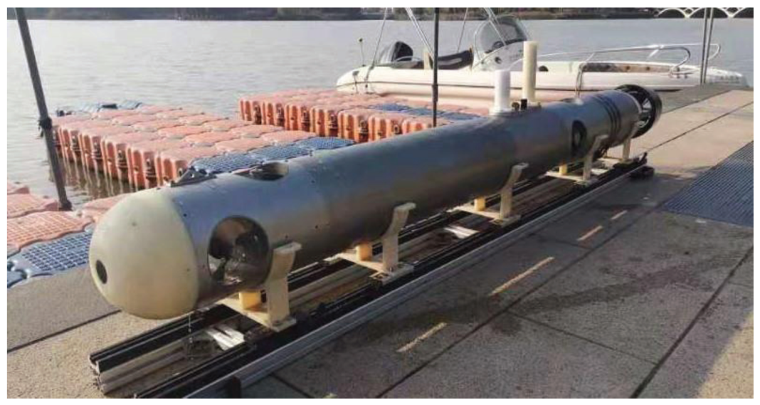
The research object of this paper is a small AUV, as shown in Figure 1. The length of the AUV is about 2200 mm and the displacement is 68 kg. The relevant configuration parameters are shown in

Table 1. Physical parameters for AUV.

AUV Parameters	Values
Size	L = 2150 mm
	H = 200 mm
	W = 200 mm
Mass	m = 68 kg
Moment of inertia	$Ix$ = 0.68 kg m${}^2$
	$Iy$ = 33 kg m${}^2$
	$Iz$ = 33 kg m${}^2$
Propeller diameter	D = 110 mm
Propeller position	$l_{bh}$ = 700 mm
	$l_{bv}$ = 550 mm
	$l_{sh}$ = −600 mm
	$l_{sv}$ = −750 mm

. One main propeller and four side propellers are mounted for maneuvering. The horizontal propeller arranged in the bow and stern is used for AUV’s heading control, while the vertical propeller is used for AUV’s depth and attitude control. The AUV is not equipped with a roll control device, and the roll stability is guaranteed through static buoyancy.

The AUV is customized for the mission of course and position control under hover or low speed state, and the research results will be applied to large underwater platform in future work. That is the reason the AUV is not equipped with rudder mechanisms.

The structure of bow propellers is shown in Figure 2. The structure of the propulsion section of the stern part is basically the same as that of the bow part. The four side thrusters are of the same size and construction. To eliminate the adverse effect of additional torque on the attitude of the underwater robot caused by the propulsion of the stern part, the rotation direction of the propellers of the stern part and the propellers of the bow part are opposite.

AUV is generally regarded as a rigid body with six degrees of freedom, and its translational and rotational equations can be established according to Newton’s laws. According to Fossen’s scheme, inertial reference frame $O\xi \eta \zeta$ and body fixed frame $oxyz$ are, respectively, established, as shown in Figure 3. Displacement $\xi ,\eta ,\zeta$ and attitude angles $\varphi ,\theta ,\phi$ are defined in inertial frames.

The linear velocity of AUV in the direction $ox,oy,oz$ is $u,v,w$, and the angular velocity is $p,q,r$, respectively. Suppose that the hydrodynamic force and the torque applied to AUV is $X,Y,Z$ and $K,M,N$, respectively. Then, the dynamic and dynamic moment equations of AUV in correspondence direction can be described as

$$\left\{\begin{array}{c}m[\dot{u}-vr+wq+z_G(pr+\dot{q})]=X\hfill \\ m[\dot{v}-wp+ur+z_G(qr-\dot{p})]=Y\hfill \\ m[\dot{w}-uq+vp-z_G(p^2+q^2)]=Z\hfill \\ I_x\dot{p}+m\left[z_G(\dot{v}-wp+ur)\right]=K\hfill \\ I_y\dot{(}q)+(I_x-Iz)rp+m\left(z_G(\dot{u}-vr+wq)\right)=M\hfill \\ I_z\dot{(}r)+(I_y-Ix)pq=N\hfill \end{array}\right.$$

(1)

where $I_x$, $I_y$, and $I_z$ are the moment of inertia in the x, y and z directions, respectively, and $z_G$ is the position of center of gravity in z direction.

In practice, the coupled dynamic equation is usually simplified into three independent subsystems: yaw, pitch, and roll. Due to the axisymmetric characteristics of the AUV, the rotational inertia of pitch direction and yaw direction are approximately the same, that is, $Iy=Iz$. We can assume that the hydrodynamic parameters of the yaw model of AUV are consistent with those of the pitch model. Therefore, the research in this paper focuses on the model parameters of yaw subsystem. The rolling motion of the slender AUV has a comparable high frequency band, and the motion has little influence on the dynamic process of the pitching subsystem and yaw subsystem, thus the rolling motion is not considered in this work. For this reason, the dynamic coefficients of roll motion are not identified in this work.

The hydrodynamic characteristics of a certain geometry propeller in open water is thrust and torque. They are related to propeller diameter, propeller speed, velocity to water, water density, water viscosity coefficient, gravitational acceleration, etc.

Based on the principle of fluid mechanics, the thrust model of each propeller is set as:

$$T=sign\left(n\right)*(1-t)\rho K_{T0}{n}^2{D}^4$$

(2)

where D is propeller diameter, n is rotation speed, $K_{T0}$ is thrust coefficient, and $\rho$ is seawater density. The function $sign\left(n\right)$ is the absolute value of the quantity of revolution. t is the thrust reduction, which is the key factor to generate the uncertainty of propeller thrust model.

The work of the propeller causes turbulence in the flow field around the AUV, thus changing the hydrodynamic model of the AUV. The propeller model is difficult to be obtained by theoretical calculation or CFD method.

The hydrodynamic forces and moments of AUV can be described as

$$\left\{\begin{array}{c}X=X_{uu}u\left|u\right|+X_{vr}vr+X_{wq}wq+(1-t_m)K_m{n}^2\hfill \\ Y=Y_{\dot{v}}\dot{v}+Y_{\dot{r}}\dot{r}+Y_{v}v+Y_{r}r+(1-t_{bh})K_t{n}_{bh}^2+(1-t_{sh})K_t{n}_{sh}^2\hfill \\ M=M_{\dot{v}}\dot{v}+M_{\dot{r}}\dot{r}+M_{v}v+M_{r}r+(1-t_{bh})K_t{l}_{bh}{n}_{bh}^2+(1-t_{sh})K_t{l}_{sh}{n}_{sh}^2\hfill \\ Z=Z_{\dot{w}}\dot{w}+Z_{\dot{q}}\dot{q}+Z_{v}v+Z_{r}r+(1-t_{bv})K_t{n}_{bv}^2+(1-t_{sv})K_t{n}_{sv}^2\hfill \\ N=N_{\dot{w}}\dot{w}+N_{\dot{q}}\dot{q}+N_{v}v+N_{r}r+(1-t_{bv})K_t{l}_{bv}{n}_{bv}^2+(1-t_{sv})K_t{l}_{sv}{n}_{sv}^2\hfill \end{array}\right.$$

(3)

The above equation includes 19 hydraulic coefficients ( $X_{*},Y_{*},X_{*},M_{*},N_{*}$), 5 thrust reduction coefficients ($t_m,t_{bh},t_{sh},t_{bv},t_{sv}$), 4 moment arm coefficients ($l_{bh},l_{sh},l_{bv},l_{sv}$), thrust coefficients $K_m$ of main propeller, and thrust coefficients $K_t$ of side propeller. The hydraulic coefficient can be obtained by CFD calculation, the thrust coefficient can be obtained by product parameters, and the moment arm length can be deduced by AUV layout.

The thrust reduction coefficient should be obtained by the identification method. When the propeller is loaded on board, the installation position of the propeller, the shape of the hull, and other propellers installed nearby affect the performance of the propeller. Meanwhile, the propeller’s work affects the flow field around hull, and the result is that both the hydrodynamic of hull and the propeller are different from when they work alone. Due to the existence of thrust reduction, it is difficult to obtain accurate and complete AUV mathematical model by CFD method.

3. Hydrodynamic Parameter Calculation Based on CFD

In our method, the rough mathematical model is firstly established by using the AUV physical parameters and CFD method, and the motion controller is designed based on rough model to realize the excitation experiment and data acquisition. The identification algorithm uses the recording data to correct the rough coefficients and improve the accuracy of the mathematical model. The schema of our method is shown in Figure 4.

In this section, CFD fluid dynamics simulation is applied to simulate the force, torque, pressure, and other physical parameters of an AUV under different rotational states, which are then substituted into the analysis model. The hydrodynamic parameters of an AUV are calculated by FLUENT ANSYS, and the shape of the AUV is shown in Figure 4. Fluent has the ability to simulate multiple physical fields. It has a wide range of applications and is currently the most complete CFD software.

The AUV is driven and operated by propellers, and the interaction between the propeller and the AUV body makes the flow field complicated, which is difficult to calculate by CFD method. Therefore, the influence of propeller is ignored in CFD calculation, and only the hydrodynamic parameters generated by AUV hull are calculated. These calculated parameters are modified by using the experiment data in the following section.

The accuracy of CFD calculation results depends on the quality of grid division, the choice of calculation mode, the setting of parameters, boundary conditions, etc.

We provide a computational domain around the vehicle body to simulate the interaction between vehicle motion and surrounding fluids, as shown in Figure 5.

Boundary conditions define the interaction between the simulation model and its environment. The convergence of CFD simulation is related to the definition of boundary conditions. In our work, an inlet boundary condition is located two body lengths upstream with inflow velocities of 0.1–0.4 m/s. Then, an outlet boundary condition with zero relative pressure is located at two body lengths downstream. Finally, the hull of AUV is the only solid boundary in the computational fluid domain and is set to a wall with a no-slip condition.

The CFD model requires that the fluid domain be divided into grids, which are composed of geometric elements such as hexahedron and tetrahedron. On this basis, the governing equation is used for discretization and solution. The distribution of these grid elements defines the level of precision.

In our work, CFD calculation provides the initial reference of model parameters, which requires relatively low accuracy of the calculation results. On the other hand, the size of AUV is large, and CFD calculation should consume a lot of calculation resources. For these reasons, in the current model, the appropriate unit size is selected to ensure that there are a sufficient number of units to parse the geometry and flow field. The refined mesh is used around the moving object to increase the mesh density and ensure that the flow field is properly set, as shown in Figure 6. In our calculation, the total number of grids is 955,815 and the number of nodes is 1,355,389. Other parameter settings include 20 mm for face size and 100 mm for body size.

Computational fluid dynamics (CFD) computes the Navier Stokes equations for fluid flow in the domain. The Navier–Stokes equations describe the dynamic equilibrium of forces acting on any given region of the liquid. These equations establish the relationship among the rate of change in momentum (acceleration) of the particles, the change in pressure acting on the inside of the fluid, and the dissipative viscous force (similar to friction) and gravity.

A suitable turbulence model should be selected to simulate the turbulence effect in the flow around the AUV hull. The commonly used turbulence models include $k-ϵ$ standard, RNG $k-ϵ$ model, SST $k-ϵ$ model, etc. Since the CFD calculation results is used as the initial reference for modeling, subsequent identification algorithms modify the calculation results. Therefore, we ch0ose the most commonly used $k-ϵ$ standard model for the consideration of computational cost and convergence. Unlike earlier turbulence models, k-epsilon model focuses on the mechanisms that affect the turbulent kinetic energy. The underlying assumption of this model is that the turbulent viscosity is isotropic. Since the main purpose of simulation is to obtain the data of force and torque parameter, we also add the change of force and torque as the convergence condition, in addition to the basic convergence condition.

Figure 7 shows the shows the continuity, velocities in x, y, z directions, the turbulent kinetic energy, and the rate of dissipation epsilon under the conditions of $u=0.1\mathrm{m}/\mathrm{s},v=0.05\mathrm{m}/\mathrm{s}$, and r = 2°/s, as well as the number of iterations. As shown in the figure, when the calculation variable are approximately unchanged, the calculation of our task converges.

Table 2. Calculation result of hydrodynamic force.

u (m/s)	v (m/s)	r (°/s)	X (N)	Y (N)	N (Nm)
0.10	0.00	0.0	−0.011151	0	0
		2.0	0.25622	−0.22266	−0.30988
		4.0	1.122	−0.42181	−1.3298
		6.0	2.2813	−0.6282	−3.1116
	0.05	0.0	0.16631	−1.9086	−0.18648
		2.0	0.39531	−2.5188	−0.46914
		4.0	1.3318	−2.6876	−1.5878
		6.0	2.4309	−2.6935	−2.9156
0.20	0.00	0.0	−2.3499	0	0
		2.0	−1.8157	−0.42188	−0.32632
		4.0	−1.0253	−0.95101	−1.3495
		6.0	0.28591	−1.2341	−3.1384
	0.05	0.0	−2.1042	−3.8827	−0.37828
		2.0	−1.7414	−4.0678	−0.69061
		4.0	−0.87193	−4.5786	−1.6169
		6.0	0.4385	−4.8503	−3.5752
0.30	0.00	0.0	−6.4166	0	0
		2.0	−5.4324	−0.71734	−0.36066
		4.0	−4.4096	−1.4029	−1.3365
		6.0	−3.2172	−1.9543	−2.7476
	0.05	0.0	−5.3079	−6.4429	−0.61755
		2.0	−5.5339	−6.0041	−0.88661
		4.0	−4.4829	−7.7136	−1.7452
		6.0	−2.9345	−7.3884	−3.6607
0.40	0.00	0.0	−11.55	0	0
		2.0	−10.862	−0.84952	−0.40854
		4.0	−9.3096	−1.8374	−1.3159
		6.0	−8.3137	−2.7235	−3.2169
	0.05	0.0	−9.9644	−8.5102	−0.79617
		2.0	−10.57	−8.6109	−1.1319
		4.0	−9.3862	−9.6247	−2.1641
		6.0	−8.9076	−11.113	−3.9105

lists the calculation results of AUV resistance, lateral force, and torque under different horizontal motion conditions. The hydrodynamic parameters of horizontal movement can be obtained by the regression of the above calculation results, which is discussed in the following section.

4. Maximum Likelihood Identification Algorithm

The above research work gives the calculation method and related results of hydrodynamic parameters of the vehicle based on CFD. However, the parameters have non-negligible errors, especially when multiple thrusters are operating simultaneously. This section discusses the parameter correction method based on CFD parameters and navigation data.

The basic principle of maximum likelihood identification is to construct a likelihood function with experiment data and unknown parameters. When the function reaches a maximum at a certain parameter value, the estimated value of system model parameters can be obtained.

4.1. Identification Principle and Process

The maximum likelihood identification algorithm is based on the model parameters of the above CFD calculation and uses the experimental data to correct the parameters, so as to obtain the mathematical model with higher consistency. The process is shown in Figure 8.

The vector of the parameters to be identified is defined as $\theta$, on which the state equation and sensitivity equation can be established. The former is used for simulating and predicting AUV motion, and the latter is used for describing the dependence of the prediction error to the model parameters. $\theta$ is first roughly estimated by CFD calculation, and then corrected by AUV experimental data.

The correction process is as follows: AUV is used to conduct experiments to obtain sensor test data, while the equation of state is used to predict the motion process under the same experimental conditions. The deviation between the two is the prediction error. The prediction error and sensitivity data are then used to synthesize the correction value $\Delta \theta$. This value is used to update the model parameter $\theta$. This correction process will reduce the model prediction error e. When prediction error e converges to a small enough value, the modified parameters are considered as the final identified parameters.

On the one hand, parameter correction based on navigation data can effectively improve the accuracy of CFD calculation parameters. On the other hand, the results of CFD calculation can be used as the initial value of model modification to ensure the convergence of identification algorithm. This identification method requires low abundance of experimental samples of voyage data, and no special voyage test experiment is needed, thus effectively reducing the modeling cost.

In the maximum likelihood identification algorithm, several concepts are involved, including mathematical model, equation of state, measurement equation, sensitivity equation, and parameter vector to be identified.

• Mathematical model: The mathematical model is described by the dynamics and kinematics equation of mass center, the dynamics and kinematics equation of vehicle motion around the center, the mass equation, and the geometric relation equation.
• State equation: Equations of dynamics and kinematics are expressed in differential form.
• Observation equation: During the motion of the vehicle, only part of the motion state can be measured, and the measurement results are mixed with measurement noise. The relationship between the true value of a state and the measured value is called the observation equation.
• Sensitivity equation: The differential equation of sensitivity is obtained by differentiating the state equation the observation equation.
• Parameters vector: Vectors are formed by the parameters to be identified.
• Initial parameter value: The initial estimate of the parameter is used to initiate the identification iteration process. Hydrodynamic parameters are obtained by CFD calculation, AUV parameters about mass, inertia and geometric refer to AUV configuration file, and propeller parameters refer to equipment description.

4.2. Equations and Parameters for Identification Algorithm

One of the key problems of the above identification methods is the convergence of the algorithm, which may be caused by the complex model form, large initial parameter deviation, and excessive sensor noise. Therefore, it is necessary to simplify the form of the identified model. Based on this consideration, the identification of vertical plane motion model and horizontal plane motion model are carried out separately in the identification experiment. That is, the AUV depth is kept unchanged and the pitch angle is controlled to be zero when the experiment of horizontal motion model identification is carried out.

For the first step, we need to determine the form of the identification model. Considering the coupling between dynamic variables, the motion equation can be decomposed into vertical motion equation and horizontal motion equation. The horizontal equation includes surge, sway, and heading dynamic, while the vertical equation includes surge, pitching, and heave dynamic. The horizontal and vertical equation can be deduced with Equations (1) and (3)

$$\left\{\begin{array}{c}m(z\dot{w}-uq)=Z_{\dot{w}}\dot{w}+Z_{\dot{q}}\dot{q}+Z_{w}w+Z_{q}q+(1-t_{bv})K_t{n}_{bv}^2+(1-t_{sv})K_t{n}_{sv}^2\hfill \\ I_y\dot{q}=M_{\dot{w}}\dot{w}+M_{\dot{q}}\dot{q}+M_{w}w+M_{q}q+(1-t_{bv})l_{bv}{K}_t{n}_{bv}^2+(1-t_{sv})l_{bv}{K}_t{n}_{sv}^2\hfill \\ m(\dot{u}+wq)=X_{uu}u\left|u\right|+X_{wq}wq+(1-t_m)K_m{n}^2\hfill \end{array}\right.$$

(4)

$$\left\{\begin{array}{c}m(\dot{v}+ur)=Y_{\dot{v}}\dot{v}+Y_{\dot{r}}\dot{r}+Y_{v}v+Y_{r}r+(1-t_{bh})K_t{n}_{bh}^2+(1-t_{sh})K_t{n}_{sh}^2\hfill \\ I_z\dot{r}=N_{\dot{v}}\dot{v}+N_{\dot{r}}\dot{r}+N_{v}v+N_{r}r+(1-t_{bh})K_t{l}_{bh}{n}_{bh}^2+(1-t_{sh})K_t{l}_{sh}{n}_{sh}^2\hfill \\ m(\dot{u}-vr)=X_{uu}u\left|u\right|+X_{vr}vr+(1-t_m)K_m{n}^2\hfill \end{array}\right.$$

(5)

The above equations constitute the state equation of state for model identification algorithm. The sensitivity equation of identification algorithm can be obtained by taking the partial derivative of the state equation (see Appendix A).

Considering the form of horizontal Equation (5), the relevant state variables include $u,v$, and r. Equation parameters include hydrodynamic parameters $X,Y,N$, propeller parameters $K_t,t_{bh},t_{sh}$, mass parameters $m,I_z$, and geometric parameters $l_{bh},l_{sh}$. The quality parameters and geometric parameters are obtained by the AUV configuration, the thrust parameter $Kt$ is obtained by the factory parameters, and other parameters need to be identified.

The initial values of coefficient $Y_v,Y_r,N_v,N_r,X_{vr},X_u$ are determined with CFD calculation. Figure 9 shows the relationship among hydrodynamic force (X, Y, N), surge, and heading velocity in Table 2. There is an obvious linear relationship among them, thus relevant parameters can be obtained by linear regression method.

The coefficients of differential hydrodynamic items are difficult to calculate. They have little influence on the hydrodynamic term, which is obtained by the following method. Reviewing the hydrodynamic coefficients of slender cylinder type AUV [18,25] and to guarantee conservative, the range of coefficient $Z_{\dot{w}}$ and $M_{\dot{q}}$ can be considered as:

$$-3m<Z_{\dot{w}}<0$$

(6)

$$-3I_y<M_{\dot{q}}<0$$

(7)

Hence, the nominal values for $Z_{\dot{w}}$ and $M_{\dot{q}}$ can be selected as the average value of above range. On the other hand, the effects of $Z_{\dot{q}}$ and $M_{\dot{w}}$ on hydrodynamic can be reasonably neglected.

To facilitate the algorithm solution, we conduct dimensionless processing of related parameters, i.e.,

$$\left\{\begin{array}{c}{X}_{uu}=X_{uu}^{\prime }·\rho ·L^2/\left(2m_x\right)\hfill \\ X_{vr}=X_{vr}^{\prime }·\rho ·L^3/\left(2m_x\right)\hfill \\ Y_v=Y_v^{\prime }·\rho ·L^2/\left(2m_y\right)\hfill \\ Y_{\dot{v}}=Y_{\dot{v}}^{\prime }·\rho ·L^3/\left(2m_y\right)\hfill \\ Y_r=Y_r^{\prime }·\rho ·L^3/\left(2m_y\right)\hfill \\ N_v=N_v^{\prime }·\rho ·L^3/\left(2I_z\right)\hfill \\ N_r=N_r^{\prime }·\rho ·L^4/\left(2I_z\right)\hfill \\ N_{\dot{r}}=N_{\dot{r}}^{\prime }·\rho ·L^5/\left(2I_z\right)\hfill \end{array}\right.$$

(8)

In this way, we establish the identification parameter vector as

$$\mathsf{\Theta }=({\theta }_1,{\theta }_2,{\theta }_3,{\theta }_4,{\theta }_5,{\theta }_6,{\theta }_7,{\theta }_8)=(Y_v^{\prime },Y_r^{\prime },t_{bh},t_{sh},N_v^{\prime },N_r^{\prime },X_{uu}^{\prime },X_{vr}^{\prime })$$

(9)

The initial values of model parameters can be obtained by using the above method, as shown in

Table 3. Initial values of coefficients.

Coefficients	Values	Coefficients	Values
$X_{uu}^{\prime }$	−0.8127	$X_{vr}^{\prime }$	2.5207
$Y_{\dot{v}}^{\prime }$	−4.9715	$N_{\dot{r}}^{\prime }$	−0.3597
$Y_v^{\prime }$	−1.0097	$N_v^{\prime }$	−1.1433
$Y_r^{\prime }$	0.0940	$N_r^{\prime }$	−0.1661
$t_{bh}$	0.25	$t_{sh}$	0.25
$t_{bv}$	0.25	$t_{sv}$	0.25
$K_t$	0.075	t	0.25

.

4.3. Identification Algorithm

The motion sensors commonly equipped in AUV include inertial navigation unit (INU) and doppler log. In this research, the GIF 65536 fiber optic inertial navigation unit and Teledyne PathFinder 600 KHz DVL are used to provide measured values of linear and angular velocity. The depth measurement accuracy of INU is 4 m (Root-Mean-Square (RMS)), attitude, and course measurement accuracy is 0.15 deg/s (RMS). The velocity measurement accuracy of DVL is 0.2% ± 0.002 m/s, and the resolution is 0.001 m/s.

The acceleration signal can be obtained by differentiating the velocity signal, but with more noise. Therefore, for the horizontal motion equation, the observation vector is selected as $y=(u,v,r)=(y_1,y_2,y_3)$, and the observation equation is

$$\left\{\begin{array}{c}\widehat{u}=u+u_n\hfill \\ \widehat{v}=v+v_n\hfill \\ \widehat{r}=r+r_n\hfill \end{array}\right.$$

(10)

where $\widehat{u},\widehat{v},\widehat{r}$ is measured value vector. $u_n,v_n,r_n$ is the measured noise, which obeys the Gaussian distribution, and the expected values are zero.

The likelihood criterion function is chosen as

$$J\left(\mathsf{\Theta }\right)=\sum _{i=1}^N{e}^T\left(i\right)B^{-1}\left(i\right)e\left(i\right)+ln\left|B\left(i\right)\right|$$

(11)

where $e\left(i\right)$ is the deviation between prediction value $y_p\left(i\right)$ and real value $y\left(i\right)$, that is $e\left(i\right)=y_p\left(i\right)-y\left(i\right)$. i denotes the number of sample data. B is the covariance matrix of the observed noise. Since the measurement $u_n,v_n,r_n$ noise is unknown, the optimal estimation value is adopted:

$$B=\widehat{B}=\frac{1}{N}\sum _{i=1}^{N}e\left(t_i\right)e^T\left(t_i\right)$$

(12)

The identification problem of hydraulic parameters is to find the estimation $\widehat{\mathsf{\Theta }}$ of identification parameter $\mathsf{\Theta }$, so as to minimize the function $J\left(\mathsf{\Theta }\right)$

$$\widehat{\mathsf{\Theta }}=argminJ\left(\mathsf{\Theta }\right)$$

(13)

The Newton–Raphson iterative algorithm is used to solve the optimization problem; the identification parameter vector $\mathsf{\Theta }$ can be updated with:

$${\mathsf{\Theta }}_{k+1}={\mathsf{\Theta }}_k+\Delta {\mathsf{\Theta }}_k$$

(14)

where the calculation of correction $\Delta {\mathsf{\Theta }}_k$ is:

$$\frac{{\partial }^{2}J}{\partial \theta \partial \theta }\Delta {\mathsf{\Theta }}_k=-\frac{\partial J}{\partial \mathsf{\Theta }}$$

(15)

Substituting Equation (10) into Equation (14), we can get eight-dimensional systems of linear equations, each with the following form:

$$\begin{array}{c}\sum _{l=1}^8\sum _{i=1}^N\left(\sum _{j=1}^3\sum _{k=1}^3\frac{\partial e_j\left(i\right)}{\partial {\theta }_l}{B}_{jk}^{-1}\frac{\partial e_k\left(i\right)}{\partial {\theta }_m}\right)\Delta {\theta }_l\\ =\sum _{i=1}^N\left(\sum _{j=1}^3\sum _{k=1}^3{e}_j\left(i\right)B_{jk}^{-1}\frac{\partial {\widehat{e}}_k\left(i\right)}{\partial {\theta }_m}\right)\end{array}$$

(16)

where i is the sampling count $j,k$ is the ordinal number of the observed variable, and l is the ordinal number of the identification parameter. The coefficients $\frac{\partial e_j\left(i\right)}{\partial {\theta }_l},\frac{\partial e_k\left(i\right)}{\partial {\theta }_m}$ are the integration of the sensitivity equation, which is obtained by differentiating the above state equation.

The execution process of the above algorithm is described as follows:

• The state Equation (5) is initialized with parameters $\mathsf{\Theta }$ estimated by empirical method or CFD, which are listed in Table 3.
• The state Equation (5), and sensitivity Equations (A1)–(A3) are integrated to obtain the prediction state value $y_p=(u_p,v_p,r_p)$ and the sensitivity function $\frac{\partial e_j\left(i\right)}{\partial {\theta }_l},\frac{\partial e_k\left(i\right)}{\partial {\theta }_m}$, respectively. The array of linear algebraic equations in Equation (15) is constructed from the prediction value, sensitivity value, and measured value $\widehat{y\left(i\right)}=(\widehat{u},\widehat{v},\widehat{r})$. The form of sensitivity function is found in the Appendix A.
• The correction $\Delta \mathsf{\Theta }=({\theta }_1,{\theta }_2,\cdots ,{\theta }_8)$ is obtained by solving Equation (15), and used for the modification of state equations, that is Equation (13).
• The modified coefficient $\mathsf{\Theta }$ is then substituted into state equation and sensitivity equation. Then, the above above process is repeated.
• The likelihood function $J_k$ of each iteration step is calculated. According to the maximum likelihood criterion, when

  $$|1-\frac{J_k}{J_{k-1}}|<ϵ(ϵ=0.01)$$

  (17)

  the iteration is considered to converge, and then $\mathsf{\Theta }$ is the result of identification.

We can establish the identification algorithm of the vertical motion equation with a similar principle.

5. Experiment and Result

In this section, the model in Equation (5) is identified using the actual voyage data of AUV. To collect the experimental data of AUV horizontal movement, the depth and trim of AUV must be controlled within a certain range. The general schema of depth and pitch controller is depicted in Figure 10.

The controller consists of two loops and the control parameters are designed based on the parameters in Table 3. In this experiment, AUV did not need to do a large range of depth maneuver, we simply decoupled the depth and trim control. The inner loop is concerned with the stability of the trim angle, and is a PD controller for stern vertical propeller. Its differentiator decreases response overshoot and adds damping and stability. The outer loop uses bow vertical thrusters to control depth. It is a typical PID controller, and its integrator removes steady state error. During the field experiment, the PID control parameters were adjusted according to PID control law to ensure that the depth deviation was within 0.2 m and the trim angle was within 0.5 degree. Since the AUV was customized for the course and position control research under hover or low speed, the speed control range was within 0.4 m/s during the experiment.

Due to the difference of propeller installation position between pitch channel and steering channel and the influence of turbulence caused by propeller, the model parameters of the two channels may have certain difference.

5.1. Identification with Stern Propeller Manipulation Data

In the first experiment, the vertical propellers were used to automatically control the depth and trim, and the stern horizontal propeller was used to drive AUV for steering. The propeller instruction was $T_{hs}=150+50sin(0.15t)+10sin\left(5t\right)$ rpm. The recorded data of INU and doppler log are shown in Figure 11 and Figure 12. In the main stage of the experiment, the depth control deviation was within 0.05 m, and the trim control deviation was within 0.3 degrees. For this reason, the hydrodynamic factors of vertical motion were very small, thus the influence of vertical motion on horizontal motion could be ignored.

The proposed identification algorithm was applied to the recorded data. The difference between the predicted surge, sway, and heading velocity in the iteration process is shown in Figure 13, and the parameter values calculated in each iteration step are given in

Table 4. Identification result of Experiment 1.

Coefficient	Iteration 1	Iteration 2	Iteration 3	Iteration 4	Iteration 5
$X_{uu}^{\prime }$	−0.7044	−0.7109	−0.7108	−0.7108	−0.7108
$X_{vr}^{\prime }$	1.7171	1.7321	1.7314	1.7314	1.7314
$Y_v^{\prime }$	−0.3315	−0.3873	−0.4541	−0.4690	−0.4668
$Y_r^{\prime }$	0.1257	0.1193	0.1141	0.1141	0.1141
$N_v^{\prime }$	−0.2938	−0.4562	−0.4805	−0.4711	−0.4707
$N_r^{\prime }$	−0.2539	−0.3361	−0.1162	−0.1162	−0.1162
$t_{hs}$	0.26	0.28	0.29	0.29	0.29
$J\left(\mathsf{\Theta }\right)$	−5.8505	−8.2006	−8.9839	−8.9648	−8.9646

.

According to the convergence criterion in Equation (17), the identification algorithm could convergence after four iterations, and the final mean square error (RMS) of surge velocity, turning velocity, and sway velocity between the mathematical model and the original data is 0.0132 m/s, 0.0028 rad/s, and 0.0113 m/s, respectively, which has a good consistency, as shown in Figure 13.

By comparing the model parameters of CFD calculation in Table 3 with the final identification parameters, it can be found that the parameters $X_{uu}$, $X_{vr}$, $Y_r$, $N_r$, and $N_v$ were more accurate than the other parameters in CFD calculation. That means CFD has a good computational performance for longitudinal resistance, but the computational accuracy of lateral force is relatively low, while there are great differences in the calculation of steering torque parameters. One possible reason is that the CFD calculation is carried out for the external structure in Figure 5, without considering the influence of bow and stern thrusters on the flow field.

5.2. Identification with Bow Propeller Manipulation Data

In the second experiment, the bow horizontal propeller was used to drive AUV for steering with instruction $T_{hb}=150+50sin(0.15t)+10sin\left(5t\right)$ rpm. The recorded data of INU and doppler log are shown in Figure 14 and Figure 15. Due to vertical thruster control, the AUV depth remained unchanged and the pitch angle was maintained as 0 degree. We can suppose that the vertical hydrodynamic factors do not affect the horizontal motion, and the proposed identification algorithm could be applied directly.

The proposed identification algorithm was applied to the recorded data. We found that the identification algorithm converged after four iterations. The difference of the predicted surge, sway, and heading velocity in the iteration process is shown in Figure 16, and the parameter values calculated in each iteration step are given in

Table 5. Identification result of Experiment 2.

Coefficient	Iteration 1	Iteration 2	Iteration 3	Iteration 4	Iteration 5
$X_{uu}^{\prime }$	−0.7913	−0.7427	−0.7227	−0.7227	−0.7227
$X_{vr}^{\prime }$	2.2515	2.2196	2.2201	2.2201	2.2201
$Y_v^{\prime }$	−0.4842	−0.3492	−0.2690	−0.2244	−0.2244
$Y_r^{\prime }$	0.0832	0.0974	0.1023	0.1023	0.1023
$N_v^{\prime }$	−0.2815	−0.5882	−0.6159	−0.6152	−0.6152
$N_r^{\prime }$	−0.3843	−0.3502	−0.1369	−0.1366	−0.1366
$t_{hb}^{\prime }$	0.25	0.25	0.25	0.24	0.24
$J\left(\mathsf{\Theta }\right)$	−6.8206	−8.7165	−8.9874	−8.9762	−8.9746

.

By comparing the experiment data with the simulation prediction data, it can be seen that the final mean square error (RMS) of surge velocity, turning velocity, and sway velocity between the mathematical model and the original data is 0.0117 m/s, 0.0025 rad/s, and 0.0107 m/s, respectively. The prediction error is roughly equal to Experiment 1. It can also be seen that $X_{uu}$, $X_{vr}$, $Y_r$, $N_r$, and $N_v$ are among the more accurate parameters for CFD calculation. This is consistent with the conclusion of Experiment 1.

It can be seen from the identification curves and data of Experiments 1 and 2 that the identification algorithm proposed in this paper has good convergence, and stable identification parameters can be obtained through at most five iterations.

Comparing the identification results of the two groups of experiments, we can see that parameters $X_{uu}^{\prime },N_r^{\prime },Y_r^{\prime }$ have a good consistency between two experiment, while there is a certain difference between the identification results of parameter $Y_v,N_v$. However, the associated hydrodynamic term of the latter parameters has a small effect on the dynamic of AUV. The main causes include the limitation of the model form, the experiment scheme, and the influence of environmental factors, including $Y_v$, which characterize the relations between lateral force and lateral movement, are greatly influenced by the wind and waves.

This parameter $Y_r^{\prime },N_r^{\prime }$ has a high consistency, which indicates that the method proposed in this paper can accurately identify turning velocity related parameters. On the other hand, the steering motion parameters are very important for AUV automatic control from the viewpoint of ship manipulation. It reflects the accuracy of the steering motion model, which is beneficial to the autonomous control of AUV, thus this method will have a good application prospect.

5.3. Model Validation

Finally, the identification parameters in Table 4 and Table 5 were used to predict the dynamic of steering process, so as to validate the consistency of the established model. In this maneuver experiment, the vertical propeller was used to automatically control the depth and trim, and the two horizontal propellers to drive AUV for steering movement. The propeller command was $T_{hs}=$ 150 rpm, $T_{hb}=50sin(0.15t)+10sin\left(5t\right)$ rpm.

The experimental data are shown in Figure 17 and Figure 18. The parameters in Table 4 and Table 5 are used to predict the motion process, and the average values in the two tables are used for the inconsistent parameters. As can be seen in Figure 18, the prediction data are in good agreement with the experimental data. It means that the identified parameters are more accurate than those of CFD calculation. However, the horizontal motion of the established model has significantly larger damping characteristics, that is, the variables in the experimental data have more oscillation. Possible causes include measurement noise, model simplification, etc.

The prediction mean square error of surge velocity, turning velocity, and sway velocity is 0.0196 m/s, 0.0031 rad/s and 0.0124 m/s, respectively. The prediction error is a little larger than the identification error in the Experiments 1 and 2. The main deviation appears in surge velocity and sway velocity, as it shows in Figure 19. The prediction error of turning velocity is relatively small; one possible explanation is that the difference in surge speed leads to the difference in turning velocity.

By comparing the predicted mean square error between the validation experiment and the convergence result of identification experiment, it can be concluded that the estimation deviation of the method proposed in this paper will be within 20%.

Due to the small deviation in the prediction of steering motion velocity, it shows again that the proposed method has a good ability in the identification and prediction of steering motion. Therefore, the modeling method proposed in this paper is valuable for automatic control of AUV.

6. Conclusions

In this work, we present a model identification method for AUVs based on CFD calculation and maximum likelihood algorithm. The research was validated with experiment results. The conclusions may be summarized as follows:

• CFD calculation results are used as the initial values of model parameters in the iterative identification process, which guarantees the convergence of the identification algorithm.
• The turbulence caused by the work of the propeller changes the flow field around AUV, increases the model uncertainty, and makes the model parameters of steering motion and pitching motion different.
• The identification accuracy of resistance coefficient and turning-related parameters is high. Other parameters, such as lateral motion, have lower identification accuracy. Generally speaking, the model established by this method has good consistency, and the model established in this method will be helpful for controller design.
• The method proposed in this paper has low experimental and computational costs, and the difference between the model prediction results and the real system is within 20%.

In this study, the model identification of AUV at relatively low speed was carried out. In the future work, the identification of the motion model and the steering model of rudder device under higher speed will be studied, and the convergence and identification accuracy of the method will be analyzed. Besides, due to the deviation in identification parameters obtained from different experimental samples, we will also study the modeling problem of uncertainty to provide better support for the control of AUVs.