Numerical Study over the Effects of a Designed Submerged Breakwater on the Coastal Sediment Transport in the Pescara Harbour (Italy)

Abstract

In 1997, in front of the Pescara Harbour (Italy), a detached breakwater was constructed. In the successive years, the sediment transport due to the combined action of waves and coastal currents, in the area between the detached breakwater and the entrance of the Pescara Harbour, produced an accumulation of about $\mathrm{40,000}{ \mathrm{m}}^3$ of sediment per year. In this paper, the causes of the accretion of the bottom elevation in front of the Pescara Harbour entrance and the effects produced by the existing detached breakwater are investigated. The effects on the sediment transport of the introduction of a new submerged breakwater designed to protect the entrance of the harbour from sediment siltation are investigated. In particular, the ability of the designed submerged breakwater, located orthogonally to the longshore current, to intercept the aforementioned solid material and to significantly reduce the accretion of the bottom in the area in front of the harbour entrance, was numerically verified. Numerical simulations were carried out by means of a model of the bottom-change composed of two sub-models: a two-dimensional phase resolving model that is used to calculate the fluid dynamic variables changing inside the wave period and a second sediment transport sub-model to simulate the bottom changes, in which the suspended sediment concentration is calculated by the wave-averaged advection–diffusion equation. The equations of motion, in which the vector and tensor quantities are expressed in Cartesian components, are written in a generalised curvilinear coordinate system. The fully nonlinear Boussinesq equations are written in an integral form and used to simulate the velocity fields.

1. Introduction

In the literature [1,2], the simulation of sea bottom changes produced by a coastal defence structure are usually carried out by simulating the hydrodynamic fields and the concentration of the suspended solid particles. In the framework of coastal sediment transport, 3D models for the simulation of the hydrodynamic fields [3,4,5,6] require considerable computational time, due to the long-time scale of the sea bottom variations. For this reason, in the context of morphodynamic simulations, the hydrodynamic equations [7,8,9,10,11,12,13] and the suspended sediment concentration equation are usually depth averaged [14].

In this context, the two-dimensional phase-resolving models, in which motion equations are not averaged over the wave period, employ the so-called Boussinesq equations, obtained with the depth integration of the motion equations and with the definition of the depth dependence of the variables. Shock-capturing schemes adopted for numerical integration of the fully nonlinear Boussinesq equations (FNBE) [15,16,17,18] allow explicit simulations of the wave propagation from deep water to the shoreline, including the wave breaking.

In the coastal regions, sea bottom modifications are caused by complex hydrodynamic processes; in these processes, the variation of the hydrodynamic quantities over the wave period causes the resuspension, transport and settling of the solid particles. The variability of the hydrodynamic field and the wave–current interactions over the wave period are taken into account in FNBE models.

The undertow is one of the phenomena that play key roles in the solid particles transport. In the undertow phenomenon, the horizontal velocities that are closest to the bottom are off-shore directed in the surf zone, while the horizontal velocities that are closest to the free-surface are on-shore directed. Lynett [19] proposed a correction to the vertical distribution of the horizontal velocity to simulate the undertow in the context of models that solve depth-averaged motion equations.

In the standard forms of FNBE, in the continuity equation, dispersive terms are present. In particular, in several works in the literature [20,21,22], located in the context of hybrid (finite volume—finite difference) numerical schemes, the dispersive term that is present in the continuity equation is discretised by means of a second-order cell-centred finite difference scheme. As demonstrated in [15], in the continuity equation, the truncation errors related to the discretisation of the dispersive term may reduce the accuracy of the numerical scheme and cause oscillations in the numerical solution. The dispersive terms in the continuity equation can be avoided by written FNBE in a proper conservative form.

In this paper, we present a simulation model for the sea bottom modifications, composed by two sub-models: the hydrodynamic modifications are simulated by means of a two-dimensional phase-resolving model that considers the variation of the variables inside the wave period and takes into account the undertow and the sea bottom modifications are simulated by means of a second sub-model that calculates the suspended sediment concentration by means of the wave-averaged advection–diffusion equation.

The motion equations and the suspended sediment concentration equations, in which the vector and tensor quantities are expressed in Cartesian components, are written in a boundary conforming generalised curvilinear coordinate system. In the region extending from deep water up to the beginning of the surf zone, the wave and hydrodynamic fields are calculated by an integral form of the FNBE; in the surf and swash region, the governing equations reduce to the nonlinear shallow water equations, in order to directly simulate the wave breaking. In the proposed model, in which the continuity equation is written in an integral form, dispersive terms are avoided. Therefore, the continuity equation is entirely discretised by a shock capturing finite volume scheme and the errors caused by the low-order discretisation of the dispersive terms are avoided.

The near-bed velocity, boundary layer thickness, friction velocity and bed shear stress are evaluated from the integration of the momentum equation over the wave boundary layer. The turbulence contribution of the wave boundary layer is considered for the evaluation of the eddy viscosity vertical distribution under breaking waves.

Following Gallerano et al. [16], the hydrodynamic numerical scheme employs genuinely 2D WENO (Weighted Essentially Non-Oscillatory scheme) reconstructions. As stated by Gallerano et al. [16], by means of this choice, it is possible to avoid numerical errors that would arise with one-dimensional reconstructions, in the context of generalised curvilinear coordinate systems.

The bottom modifications are calculated whereby the advection–diffusion equation for the suspended sediment concentration. The advective sediment transport terms in the advection–diffusion equation are formulated by using a quasi-three-dimensional (Q3D) approach [23,24].

The depth integration of the product of the horizontal velocity and the concentration vertical distribution allows calculating the advective sediment transport terms and taking into account the sediment transport related to the undertow. To calculate the bottom elevation variation over time, the spatial variation of the bed load transport and the product between the settling velocity and the difference between reference and actual sediment concentration (i.e., the concentration at a given distance from the sea bottom) are used.

The proposed model for the simulation of the sea bottom changes was applied to the abovementioned case study of the Pescara Harbour (Italy). In this paper, the effectiveness of a submerged breakwater designed to protect the entrance of the Pescara Harbour from sediment siltation is investigated by the proposed numerical model.

The present work is structured as follows. In Section 2, the hydrodynamic model and morphodynamic model are presented. In Section 3, we present the case study of Pescara Harbour (Italy). In Section 4, the discussion of the results is presented. The conclusions of the study are drawn in Section 5. At the end of the paper, there are appendices.

2. Motion Equations

2.1. Hydrodynamic Model

Let $h$ be the local still water depth and $\eta$ be the free-surface elevation with respect to the still free surface. Let $H=h+\eta$ be the total local water depth.

The fundamental idea at the basis of the Boussinesq equations is the elimination of the vertical coordinate from the flow equations and retaining some of the effects of the vertical structure of the flow. The mathematical procedure commonly used in the standard Boussinesq approximation is based on the assumption of irrotational flow and can be summarised by the following steps. A Taylor expansion is made of the horizontal and vertical velocity around a certain elevation. The Taylor expansion is truncated to a finite number of terms. The conservation of mass for an incompressible flow and the zero-curl condition are used to replace vertical partial derivatives of hydrodynamic quantities in the Taylor expansion with horizontal partial derivatives.

In the recent literature, to extend the applicability of the Boussinesq-type models to the surf zone, as well as to simulate the breaking-generated, horizontal, rotational flow, some authors derived new form of the Boussinesq equations by a procedure that allows taking into account the vertical vorticity [20,21,22]. In fact, as demonstrated in [21,22], fully nonlinear Boussinesq equations derived from the assumption of potential flow can be readily converted to equations that allow for the partially rotational flow with vertical vorticity. Wei et al. [20] retained the leading-order vertical vorticity in their equations. Chen et al. [21] and Chen [22] improved the model of Wei et al. [20] to obtain the conservation of vertical vorticity correct to second order.

Let $z$ be the vertical coordinate. Let us employ a Taylor expansion of the velocity about an arbitrary distance from the still water surface; by assuming zero horizontal vorticity, the vertical distribution of the Cartesian based horizontal velocity $\overrightarrow{U}\left(z\right)$ can be written as

$$\overrightarrow{U}\left(z\right)={\overrightarrow{u}}^{+}+\overrightarrow{v}\left(z\right)$$

(1)

where ${\overrightarrow{u}}^{+}$ is the Cartesian based horizontal velocity at the chosen arbitrary distance $\sigma$ from the still free surface and $\overrightarrow{v}\left(z\right)$ is defined in Appendix A.

Let $\overrightarrow{\overline{v}}$ be the Cartesian based depth averaged value of $\overrightarrow{v}\left(z\right)$. In this paper, the conserved variables are chosen in order to have no dispersive term in the mass conservation equation; therefore, the conserved variables are $H$ and $\overrightarrow{M}$, where $\overrightarrow{M}$ is given by

$$\overrightarrow{M}=H\left({\overrightarrow{u}}^{+}+\overrightarrow{\overline{v}}\right)$$

(2)

in which $\left({\overrightarrow{u}}^{+}+\overrightarrow{\overline{v}}\right)$ is the depth averaged horizontal velocity. We define the symbol $·$ as the scalar product in a Cartesian coordinate system. Let $L$ be the contour line of the surface element of area $\mathsf{\Delta }A$ and $\overrightarrow{n}$ the outward normal to the line $L$. By using the aforementioned choice of conserved variables, the integral form of the continuity equation reads

$${{\displaystyle \iint }}_{\mathsf{\Delta }A}\frac{\partial H}{\partial t}dA+{{\displaystyle \int }}_L\overrightarrow{M}·\overrightarrow{n} dL=0$$

(3)

Let $\nabla$ be the two-dimensional differential operator defined as $\nabla =\left(\partial /\partial x,\partial /\partial y\right)$ in a Cartesian coordinate system. We define the symbol $\otimes$ as the outer product in a Cartesian coordinate system. Let $G$ be the gravity acceleration and $\overrightarrow{R}$, $\overrightarrow{V}$, $\overrightarrow{T}$ and $\overrightarrow{W}$ be, respectively, the bottom resistance term, dispersive terms obtained by retaining terms of order $O({\mu }^2$,${\epsilon }^3{\mu }^2)$ in power series expansion and a term related to the second-order approximation of the vertical vorticity. $\overrightarrow{V}$, $\overrightarrow{T}$ and $\overrightarrow{W}$ are defined in Appendix B. It has to be noted that Equation (3) does not contain any dispersive term since the second term of the left-hand side of Equation (3) is expressed as a flux term. For this reason, the continuity equation can be discretised entirely by a high order shock capturing finite volume scheme. With this choice of conserved variables, the integral form of the momentum equation reads

$$\begin{gathered} {{\displaystyle \iint }}_{\mathsf{\Delta }A}\frac{\partial \overrightarrow{M}}{\partial t}dA+{{\displaystyle \iint }}_{\mathsf{\Delta }A} \nabla ·\left(\frac{\overrightarrow{M}\otimes \overrightarrow{M}}{H}\right)dA=-{{\displaystyle \iint }}_{\mathsf{\Delta }A}GH \nabla \eta dA-{{\displaystyle \iint }}_{\mathsf{\Delta }A}H\left(\overrightarrow{V}+\overrightarrow{T}+\overrightarrow{W}+\overrightarrow{R}\right)dA \\ -{{\displaystyle \iint }}_{\mathsf{\Delta }A}H\left(\frac{\partial \overrightarrow{\overline{v}}}{\partial t}+{\overrightarrow{u}}^{+}·\nabla \overrightarrow{\overline{v}}+\overrightarrow{\overline{v}}·\nabla {\overrightarrow{u}}^{+}+\overrightarrow{\overline{v}}·\nabla \overrightarrow{\overline{v}}\right)dA \end{gathered}$$

(4)

We define ${\eta }_c$ as an arbitrary constant value. In this paper, to obtain a “well-balanced” numerical scheme, the surface gradient term is decomposed as follows

$$GH\nabla \eta =\nabla \left(G\frac{H^2}{2}\right)-G\left(\eta -{\eta }_c\right)\nabla h-G{\eta }_c\nabla h-G\nabla \left(\frac{h^2}{2}\right)$$

(5)

In presence of irregular seabed, this decomposition ensures a balance between flux and source terms and allows the numerical scheme to satisfy the C-Property.

Furthermore, the term $\overrightarrow{V}$ on the right-hand side of Equation (4) is rewritten as follows

$$\overrightarrow{V}=\frac{\partial {\overrightarrow{V}}^{\prime }}{\partial t}+{\overrightarrow{V}}^{″}$$

(6)

where ${\overrightarrow{V}}^{\prime }$ and ${\overrightarrow{V}}^{″}$ are defined in Appendix C.

Let us define an auxiliary variable $\overrightarrow{D}$

$$\overrightarrow{D}=H\left({\overrightarrow{u}}^{+}+{\overrightarrow{V}}^{\prime }\right)$$

(7)

Let $x_l=x_l\left({\xi }_1,{\xi }_2\right)$ (with $l=1,2$) be a transformation from the Cartesian coordinate system $\overrightarrow{x}$ to a curvilinear one $\overrightarrow{\xi }$. Let ${\overrightarrow{g}}_{\left(l\right)}=\partial \overrightarrow{x}/\partial {\xi }_l$ be the covariant base vectors and ${\overrightarrow{g}}^{\left(l\right)}=\partial {\xi }_l/\partial \overrightarrow{x}$ be the contravariant base vectors. The metric tensor and its inverse are given, respectively, by $g_{lm}={\overrightarrow{g}}_{\left(l\right)}·{\overrightarrow{g}}_{\left(m\right)}$ and $g^{lm}={\overrightarrow{g}}^{\left(l\right)}·{\overrightarrow{g}}^{\left(m\right)}$ (with $m=1,2$). The Jacobian of the transformation is $\sqrt{g}=\sqrt{det\left(g_{lm}\right)}$. Let $g_{x_j}^{\left(\mu \right)}$ be the Cartesian based component projected onto the $x_j$-axis of the contravariant base vector ${\overrightarrow{g}}^{\left(\mu \right)}$. Let $f_{x_i}$ be the Cartesian based component projected onto the $x_i$-axis (with $i=1,2$) of the generic vector $\overrightarrow{f}$.

Let $\mathsf{\Delta }A=\mathsf{\Delta }{\xi }_1\mathsf{\Delta }{\xi }_2$ be the generic surface element. $\mathsf{\Delta }{\xi }_{\mu +}$ and $\mathsf{\Delta }{\xi }_{\mu -}$ ($\mu =1,2$ are cyclic) are the contour line of the area $\mathsf{\Delta }A$ on which ${\xi }_{\mu }$ is constant and which are located at the larger and at smaller value of ${\xi }_{\mu }$, respectively. Let $D_{x_i}$ be the Cartesian based component projected onto the $x_i$-axis of the vector $\overrightarrow{D}$. We indicate by the mark $\left[\widehat{}\right]$ the cell averaged of the point values. The variable ${\widehat{D}}_{x_i}$ is the cell averaged component of the vector $\overrightarrow{D}$ projected onto $x_i$-axis

$${\widehat{D}}_{x_i}=\frac{1}{\mathsf{\Delta }A}{{\displaystyle \iint }}_{\mathsf{\Delta }A}{D}_{x_i} dA$$

(8)

Let $\widehat{H}$ be the cell average value of $H$ given by

$$\widehat{H}=\frac{1}{\mathsf{\Delta }A}{{\displaystyle \iint }}_{\mathsf{\Delta }A}HdA$$

(9)

By using Equations (5) and (7) and the chain rules [25] that transform the Cartesian based differential operators in the differential operators defined in a generalised curvilinear coordinate system, Equation (4) can be rewritten as

$$\begin{gathered} \frac{\partial {\widehat{D}}_{x_i} }{\partial t}=\frac{1}{\mathsf{\Delta }A}\left\{-{\displaystyle \sum }_{\mu =1}^2\left[{{\displaystyle \int }}_{\mathsf{\Delta }{\xi }_{\mu +}}\left(\frac{M_{x_i}{M}_{x_j}}{H}\right.\right.\right.g_{x_j}^{\left(\mu \right)}+\left.G\frac{H^2}{2}{g}_{x_i}^{\left(\mu \right)}\right)\sqrt{g}d{\xi }_{\nu }- \\ \left.{{\displaystyle \int }}_{\mathsf{\Delta }{\xi }_{\mu -}}\left(\frac{M_{x_i}{M}_{x_j}}{H}{g}_{x_j}^{\left(\mu \right)}+G\frac{H^2}{2}{g}_{x_i}^{\left(\mu \right)}\right)\sqrt{g}d{\xi }_{\nu }\right]+ \\ {{\displaystyle \iint }}_{\mathsf{\Delta }A}G\left(\eta -{\eta }_c\right)\left(\frac{\partial h}{\partial {\xi }^m}{g}_{x_i}^{\left(m\right)}\right)\sqrt{g}d{\xi }_{1}d{\xi }_2+G{\eta }_c{\displaystyle \sum }_{\mu =1}^2\left[{{\displaystyle \int }}_{\mathsf{\Delta }{\xi }_{\mu +}}h{g}_{x_i}^{\left(m\right)}\sqrt{g}d{\xi }_{\nu }\right.-\left.{{\displaystyle \int }}_{\mathsf{\Delta }{\xi }_{\mu -}}h g_{x_i}^{\left(m\right)}\sqrt{g}d{\xi }_{\nu }\right]+ \\ \frac{G}{2}{\displaystyle \sum }_{\mu =1}^2\left[{{\displaystyle \int }}_{\mathsf{\Delta }{\xi }_{\mu +}}{h}^2{g}_{x_i}^{\left(\mu \right)}\sqrt{g}d{\xi }_{\nu }\right.-\left.{{\displaystyle \int }}_{\mathsf{\Delta }{\xi }_{\mu -}}{h}^2{g}_{x_i}^{\left(\mu \right)}\sqrt{g}d{\xi }_{\nu }\right]- \\ {{\displaystyle \iint }}_{\mathsf{\Delta }A}H{V}_{x_i}^{″}\sqrt{g}d{\xi }_{1}d{\xi }_2-{{\displaystyle \iint }}_{\mathsf{\Delta }A}H\left(T_{x_i}+W_{x_i}+R_{x_i}\right)\sqrt{g}d{\xi }_{1}d{\xi }_2+ \\ {{\displaystyle \iint }}_{\mathsf{\Delta }A}\frac{\partial H}{\partial t}\left(V_{x_i}^{\prime }-{\overline{v}}_{x_i}\right)\sqrt{g}d{\xi }_{1}d{\xi }_2+{{\displaystyle \iint }}_{\mathsf{\Delta }A}H{u}_{x_j}^{+}\left(\frac{\partial {\overline{v}}_{x_j}}{\partial {\xi }_m}{g}_{x_i}^{\left(m\right)}\right)\sqrt{g}d{\xi }_{1}d{\xi }_2+ \\ {{\displaystyle \iint }}_{\mathsf{\Delta }A}H{\overline{v}}_{x_j}\left(\frac{\partial u_{x_j}^{+}}{\partial {\xi }_m}{g}_{x_i}^{\left(m\right)}\right)\sqrt{g}d{\xi }_{1}d{\xi }_2+\left.{{\displaystyle \iint }}_{\mathsf{\Delta }A}H{\overline{v}}_{x_j}\left(\frac{\partial {\overline{v}}_{x_j}}{\partial {\xi }_m}{g}_{x_i}^{\left(m\right)}\right)\sqrt{g}d{\xi }_{1}d{\xi }_2\right\} \end{gathered}$$

(10)

The integral form of the continuity Equation (6) reads

$$\frac{\partial \widehat{H}}{\partial t}=-\frac{1}{\mathsf{\Delta }A}{\displaystyle \sum }_{\mu =1}^2\left[{{\displaystyle \int }}_{\mathsf{\Delta }{\xi }_{\mu +}}{M}_{x_j}{g}_{x_j}^{\left(\mu \right)}\sqrt{g}d{\xi }_{\nu }-{{\displaystyle \int }}_{\mathsf{\Delta }{\xi }_{\mu -}}{M}_{x_j}{g}_{x_j}^{\left(\mu \right)}\sqrt{g}d{\xi }_{\nu }\right]$$

(11)

Equations (10) and (11), in which the vector and tensor quantities are expressed in Cartesian components, are a novel integral form of the fully nonlinear Boussinesq equations written in a generalised curvilinear coordinate system. Equations (10) and (11) are accurate to $O\left({\mu }^2,{\epsilon }^3{\mu }^2\right)$ for the dispersive terms and conserve vertical vorticity with a leading-order error of $O\left({\mu }^4\right)$. In Equations (10) and (11) the conserved variables are $H$ and $\overrightarrow{M}$. Therefore, the momentum equation is different from the one presented by Cannata et al. [16] and, unlike Gallerano et al. [16], the continuity equation does not contain dispersive terms. This allows us to entirely discretise the continuity equation by means of a high-order shock capturing finite volume scheme. By doing so, errors in the numerical solution due to the discretisation of the dispersive term in the continuity equation, are avoided. The surface gradient term has been rewritten, in order to discretise it by a finite volume technique and obtain a "well balanced" numerical scheme.

Lynett [19] proposed a correction to the vertical distribution of the horizontal velocity calculated by depth-averaged motion equations (${\overrightarrow{u}}^{+})$, in order to represent the undertow phenomenon. Let ${\overrightarrow{u}}_B\left(z\right)$ be the corrective velocity vector [19]. The horizontal velocity $\overrightarrow{u}\left(z\right)$ is given in Appendix D.

$\mathsf{\Omega }\left(t\right)$ is the thickness of the boundary layer, $U_{\mathsf{\Omega }}\left(t\right)$ is the horizontal velocity at the top of the wave boundary layer and $u_f\left(t\right)$ is the friction velocity. $\widetilde{u_{fc}}$ is the current friction velocity and it can be found in Appendix E. By integrating the momentum equation in the boundary layer and from the logarithmic law of the velocity profile, we calculate: $\mathsf{\Omega }\left(t\right)$, $U_{\mathsf{\Omega }}\left(t\right)$, $u_f\left(t\right)$ and $\widetilde{u_{fc}}$. We indicate by the mark $\left[\tilde{}\right]$ the wave average over the wave period $T$ of the instantaneous quantities. This calculus procedure is shown in Appendix E.

The eddy viscosity, within the boundary layer, is given by

$${\nu }_{t,r}\left(z,t\right)=K{u}_f\left(t\right)z\left[1-\frac{z}{\mathsf{\Omega }\left(t\right)}\left(1-\frac{\widetilde{u_{fc}}}{u_f\left(t\right)}\right)\right]\left(1-\frac{z}{\tilde{H}}\right)$$

(12)

The eddy viscosity, outside the boundary layer, is given by

$${\nu }_{t,r}\left(z\right)=\widetilde{u_{fc}}Kz\left(1-\frac{z}{\tilde{H}}\right)$$

(13)

With breaking waves, the turbulence is produced by the current, the wave boundary layer and the wave breaking. Let $l$ be the turbulence length scale, $k_t=k_t\left(z,t\right)$ the turbulent kinetic energy induced by the wave breaking and $c_d$ equal to $0.08$. The kinetic energy production $P_k$ is evaluated according to Deigaard et al. [26]. In the calculation of the eddy viscosity ${\nu }_{t,f}\left(z,t\right)$ related to the wave breaking, the turbulent kinetic energy equation by Deigaard et al. [26] is considered

$$\frac{\partial k_t}{\partial t}=\frac{P_k}{\rho }-c_d\frac{k_t{}^{\frac{3}{2}}}{l}+\frac{\partial }{\partial z}\left({\nu }_{t,f}\left(z,t\right)\frac{\partial k_t}{\partial z}\right)$$

(14)

The value of $k_t$, obtained with Equation (14), is used to evaluate the eddy viscosity produced by the wave breaking, as follows

$${\nu }_{t,f}\left(z,t\right)=l\sqrt{k_t}$$

(15)

The total eddy viscosity ${\nu }_t\left(z,t\right)$ can be defined as the quadratic sum of two terms: the eddy viscosity related to the current and wave breaking and the eddy viscosity produced by the wave boundary layer. Therefore, ${\nu }_t\left(z,t\right)$ is evaluated as follows

$${\nu }_t{}^2\left(z,t\right)={\nu }_{t,r}{}^2\left(z,t\right)+{\nu }_{t,f}{}^2\left(z,t\right)$$

(16)

By solving the system of equations composed by Equations (10) and (11), we obtain the cell averaged value $\widehat{H}$ and the cell averaged value ${\widehat{\overrightarrow{u}}}^{+}$. By introducing WENO reconstructions, we obtain the point values $H$ and ${\overrightarrow{u}}^{+}$. By using these point values, we obtain the vertical distribution of the horizontal velocity $\overrightarrow{u}\left(z\right)$. By using $u_f\left(t\right)$, we obtain the current friction velocity $\widetilde{u_{fc}}$. From Equations (12) and (13), the vertical distribution of the eddy viscosity, ${\nu }_{t,r}\left(z\right)$, is calculated inside and outside the boundary layer. The turbulent kinetic energy is calculated by Equation (14). The eddy viscosity produced by the wave breaking, ${\nu }_{t,f}\left(z,t\right)$, is calculated by Equation (15). By using ${\nu }_{t,r}\left(z\right)$ and ${\nu }_{t,f}\left(z,t\right)$ in Equation (16), we obtain the total eddy viscosity ${\nu }_t\left(z,t\right)$.

The instantaneous values of $\overrightarrow{u}\left(z\right)$, $u_f$, ${\nu }_t$ and $H$ are used as input variables of the morphodynamic model that is shown in Section 2.2.

2.2. Morphodynamic Model

Let $C \left(z\right)$ be the wave-averaged value of the suspended solid concentration. Let the mark $\left[\overline{}\right]$ indicate the depth averaged of quantities. Let $\overline{C}$ be the depth averaged of $C \left(z\right)$, defined as

$$\overline{C}=\frac{1}{\tilde{H}}{{\displaystyle \int }}_a^{\tilde{H}}C \left(z\right) dz$$

(17)

where $a$ is a distance from the bottom which delimits the bed load transport region. Moreover, let $\widehat{\overline{C}}$ be the cell average value of $\overline{C}$. $\tilde{H}$ is the wave-averaged value of $H$ and $\tilde{\widehat{H}}$ is the wave-averaged value of $\widehat{H}$.

In the context of a quasi-three-dimensional methodology, the integral form of the solid particle concentration equation, expressed in a generalised curvilinear coordinate system, reads

$$\begin{gathered} \frac{\partial \widehat{\overline{C} }\tilde{\widehat{H}}}{\partial t}+\frac{1}{\mathsf{\Delta }A}{\displaystyle \sum }_{\mu =1}^2\left[{{\displaystyle \int }}_{\mathsf{\Delta }{\xi }_{\mu }+}{{\displaystyle \int }}_a^{\tilde{H}}C \left(z\right) {\tilde{u}}_{x_j}\left(z\right)g_{x_j}^{\left(\mu \right)}\sqrt{g}d{\xi }_{\nu }-{{\displaystyle \int }}_{\mathsf{\Delta }{\xi }_{\mu }-}{{\displaystyle \int }}_a^{\tilde{H}}C \left(z\right) {\tilde{u}}_{x_j}\left(z\right)g_{x_j}^{\left(\mu \right)}\sqrt{g}d{\xi }_{\nu }\right] \\ -\frac{1}{\mathsf{\Delta }A}{\displaystyle \sum }_{\mu =1}^2\left[{{\displaystyle \int }}_{\mathsf{\Delta }{\xi }_{\mu }+}\left({\overline{\tilde{\nu }}}_t\tilde{H}\frac{\partial \overline{C}}{\partial {\xi }_m}{g}_{x_j}^{\left(m\right)}\right)g_{x_j}^{\left(\mu \right)}\sqrt{g}d{\xi }_{\nu }-{{\displaystyle \int }}_{\mathsf{\Delta }{\xi }_{\mu }-}\left({\overline{\tilde{\nu }}}_t\tilde{H}\frac{\partial \overline{C}}{\partial {\xi }_m}{g}_{x_j}^{\left(m\right)}\right)g_{x_j}^{\left(\mu \right)}\sqrt{g}d{\xi }_{\nu }\right] \\ ={{\displaystyle \iint }}_{\mathsf{\Delta }A}(P-De)\sqrt{g}d{\xi }_{1}d{\xi }_2 \end{gathered}$$

(18)

In Equation (18), ${\tilde{u}}_{x_j}\left(z\right)$ is the wave-averaged Cartesian component projected onto the $x_j$-axis of the vector $\overrightarrow{u}\left(z\right)$, ${\overline{\tilde{\nu }}}_t$ is the wave- and depth-averaged total eddy viscosity, $De$ is the rate of the sediment deposition and $P$ is the rate of turbulent sediment pick-up. Let $C_a\left(t\right)$ and $C_R\left(t\right)$ be, respectively, the actual concentration and reference concentration. We define ${\widetilde{C }}_a$ and ${\widetilde{C }}_R$ as the wave-averaged value of the actual and reference concentration, evaluated at height from the bottom $a=2d_{50}$ ($d_{50}$ is the sediment mean diameter). ${\tilde{C}}_R$ is evaluated in Appendix F.

$De$ and $P$ are given by

$$De=w_{sed}{\widetilde{C }}_a$$

(19)

$$P=w_{sed}{\widetilde{C }}_R$$

(20)

In Equations (19) and (20), $w_{sed}$ is the sediment fall velocity.

To solve Equation (18), the solutions of Equations (19) and (20) are needed. Let ${\tilde{\nu }}_t \left(z\right)$ be the wave-averaged value of the total eddy viscosity ${\nu }_t\left(z\right)$. The value of ${\widetilde{C }}_a$ is taken as the lower boundary condition of the turbulent suspended sediment diffusion equation, defined as follows

$$-C \left(z\right) w_{sed}={\tilde{\nu }}_t\left(z\right)\frac{\partial C \left(z\right) }{\partial z}$$

(21)

and as lower extreme of the integral that gives the depth-averaged value, $\overline{C}$, defined by Equation (17). An iterative procedure is used to calculate ${\tilde{C}}_a$, using Equation (17), in which the values of ${\tilde{\nu }}_t\left(z\right)$ and $\overline{C}$ are known from the previous time step.

The total sediment transport is evaluated as the sum of the suspended load transport and of the bed load transport, which takes into account the near bed transport mechanism. Let $p$ be the sediment porosity, $z_f$ the bottom elevation, and ${({\tilde{q}}_b)}_{x_j}$ the Cartesian based component projected onto the $x_j$-axis of the bed load transport vector ${\tilde{\overrightarrow{q}}}_b$, which is the wave-averaged value of ${\overrightarrow{q}}_b$. The ${\overrightarrow{q}}_b$ equation can be found in Appendix G. The equation of the bottom modification over time, expressed in a generalised curvilinear coordinate system, reads

$$\frac{\partial z_f}{\partial t}=-\frac{1}{1-p}\left[\left(P-De\right)+\left(\frac{1}{\sqrt{g}}\frac{\partial {({\tilde{q}}_b)}_{x_j} g_{x_j}^{\left(l\right)}\sqrt{g}}{\partial {\xi }^l}\right)\right]$$

(22)

A sequence of five steps schematises the way in which the wave and current model is coupled with the model for the simulation of the bottom changes:

(1)

The instantaneous hydrodynamic quantities are computed by the hydrodynamic model presented in Section 2.1. The simulation time has a duration of about $150$ times the mean wave period.

(2)

The instantaneous hydrodynamic quantities obtained by Step 1 are averaged over the period $T^{*}$ (which is $150$ mean wave periods [27]).

(3)

The wave-averaged hydrodynamic quantities obtained by Step 2 are used as input for the solid particles’ concentration in Equation (18). Equation (18) is numerically integrated and gives the suspended sediment concentration $\widehat{\overline{C} }$.

(4)

The concentration values $\widehat{\overline{C} }$ (that are depth and wave averaged) are used to compute (by WENO reconstructions) $\overline{C}$ and the values wave-averaged actual concentration ${\widetilde{C }}_a$.

(5)

The wave-averaged reference concentration ${\tilde{C}}_R$ (computed by Step 1), the wave-averaged actual concentration ${\tilde{C}}_a$ (computed by Step 4) and the bed load transport ${\tilde{\overrightarrow{q}}}_b$ are used as input for the equation of the bottom modification (Equation (22)). We define the time step of the integration of the bed change equation as “morphological time step”. By numerically integrating Equation (22), it is possible to update the bathymetry for the successive morphological time step. The morphological time step is greater than the simulation time interval of the hydrodynamic model. The morphological time step is evaluated, by means of a trial-and-error procedure, by a posteriori verifying the numerical results.

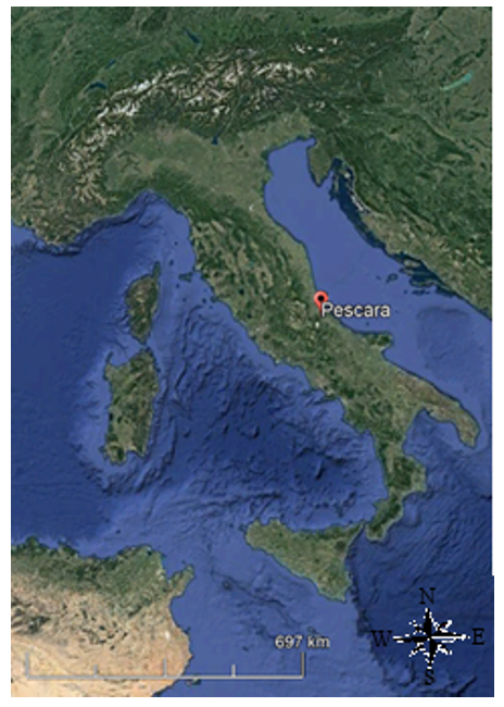
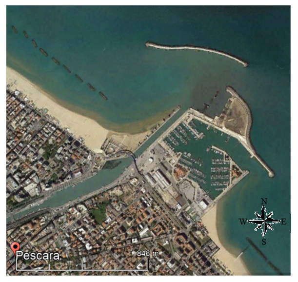
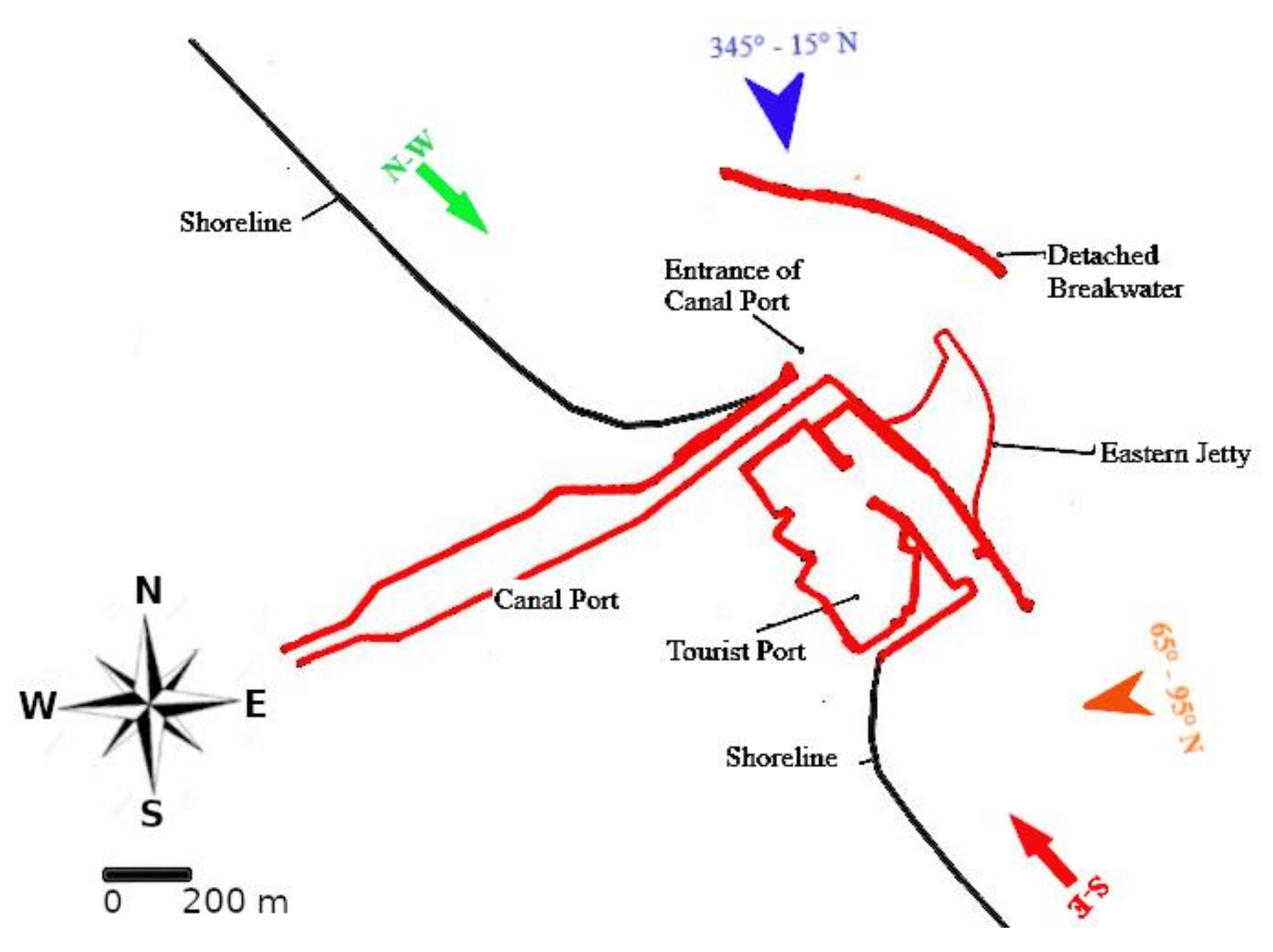
3. Pescara Harbour Case Study

The case study of the Pescara Harbour, located at the mouth of the homonymous river, represents an example of how coastal structures can modify the nearshore current patterns and consequently the sediment transport and siltation phenomena.

The Pescara Harbour is located in the central Italy and overlooks the Adriatic Sea, as shown in Figure 1.

Figure 2 shows a satellite view of the Pescara Harbour coastal area.

Figure 3 shows a schematisation of the present configuration of this coastal area. It is characterised by the presence of two ports: the Canal Port and the Touristic Port. The Canal Port is located along the terminal part of the Pescara River. The Touristic Port is located southeast of the entrance of the Canal Port. A detached breakwater is present in front of the entrance of the Canal Port.

The preeminent directions of the incoming waves representative of Pescara annual wave climate [28] are shown in Figure 3. In this figure, it is possible to notice that there are two preeminent directions: $345° \mathrm{N}–15° \mathrm{N}$ (primary sector) and $65° \mathrm{N}–95° \mathrm{N}$ (secondary sector). The primary sector incoming waves (blue arrow) produce a longshore current coming from the northwest direction (green arrow) and the sediment transport produced by the above current comes from the same direction. The secondary sector incoming waves (orange arrow) produce a longshore current coming from the southeast direction (red arrow) and a sediment transport coming from the same direction. Thus, the potential sediment transport is bimodal and the total resultant is directed from northwest to southeast.

The wave fronts coming from north direction (before the construction of the detached breakwater) caused the navigation to be difficult at the entrance of the Canal Port. To protect the entrance of the Canal Port from the wave motion and ensure good navigability conditions, in 1997, the detached breakwater was built. After the construction of the detached breakwater, a significant increase of the sea bottom level has occurred in the area in the front of the entrance of the Canal Port. The impact of the abovementioned detached breakwater on the bottom modifications in front of the entrance of the Canal Port is negative. The wave motion coming from north direction induces longshore currents coming from northwest direction. The solid material, put into suspension by the wave breaking, is transported by the longshore current into the area in front of the entrance of Canal Port. In this area, the energy of the wave motion is consistently damped by the presence of the detached breakwater. Consequently, the solid material silts near the entrance of the Canal Port, where it produces an increment of the sea bottom level and makes it difficult to navigate. The sediment transport coming from southeast is mostly intercepted by the Touristic Port and by the Eastern Jetty, before reaching the proximity of the entrance of the Canal Port. Consequently, the solid material coming from southeast does not significantly contribute to the silting of the area in front of the Canal Port. The silting of this area is due, in minor part, also to the sediment transport coming from the Pescara River during flood events.

In summary, the area in front of the entrance of the Canal Port, bounded by the detached breakwater, the Eastern Jetty and the Touristic Port, undergoes a process of silting, mainly caused by the sediment transport coming from northwest. The access to the Canal Port, in absence of periodic appropriate dredging operations, is prevented in the northwest harbour gate, due to the formation of extended areas with still water depth less than 1 m. The access to the Canal Port is possible, with difficulty, only by routes approaching the entrance from east-northeast and only by vessels with draft less than 2 $\mathrm{m}$.

In Section 3.1, we present the numerical simulations carried out to validate the hypothesis that the solid material put into suspension by the wave breaking is transported by the longshore current coming from northwest and silts near the entrance of the Canal Port.

Recently, the Italian Ministry of Public Works has considered the possible construction of a submerged breakwater that is able to act as an obstacle to the flow of solid material carried by the longshore current coming from northwest. Such solid material, as demonstrated in the present paper, settles to the northwest of the submerged breakwater. The reasons at the basis of the decision to verify the functionality of the submerged breakwater lie in the fact that (in the present configuration, without the submerged breakwater) the solid material coming from northwest mixes with the one coming from the Pescara River and settles in front of the entrance of the Canal Port, by increasing the sea bottom level. The sediment coming from northwest is generally of good quality, while the one coming from the Pescara River is polluted. The continuous dredging that should be done in front of the entrance of the Canal Port would not provide good quality sediment to be used for possible beach nourishment. According to the Italian legislation, the polluted dredged sediment must be treated, with consequent very high costs. The presence of the submerged breakwater should block the pollution-free sediment coming from northwest, which could be used for the nourishment of the touristic beach at the northwest of the submerged breakwater. Furthermore, as stated above, the submerged breakwater, by blocking the sediment coming from northwest, would limit the increase of sea bottom level at the entrance of the Canal Port, which is mainly due to sediment carried by the above mentioned longshore current. Another design solution, which consists in the construction of a system of long groins that are perpendicular to the shoreline and placed on the northwest side of the Canal Port entrance, has been considered. This solution has been rejected by the Italian Ministry of Public Works after a cost–benefit analysis because it is too expensive and is characterised by a main environmental impact.

In Section 3.2, we present the results of the investigation over the effectiveness of the introduction, in the coastal area of the Pescara Harbour (Italy), of the submerged breakwater.

Figure 4a shows the present configuration (Configuration 1), in which there is only the detached breakwater (drawn in red). Figure 4b shows the designed configuration (Configuration 2), in which the submerged breakwater (drawn in yellow) connects the detached breakwater to the shoreline. The dimensions of the submerged breakwater are: crest width equal to $3 \mathrm{m}$, larger base equal to $23 \mathrm{m}$ and slope of banks equal to $1:2$. The maximum depth where the breakwater is placed is equal to $5 \mathrm{m}$ and the freeboard is equal to $0.5 \mathrm{m}$. The submerged breakwater is modelled as a bottom increase. In both figures, the still water depth measured from mean water level is reconstructed based on bathymetric data which have been obtained after dredging operations. The still water depth in Figure 4 (measured from mean water level) is assumed as initial conditions for the simulations.

The primary sector incoming waves are characterised by a significant wave height of $1.5 \mathrm{m}$, which has an occurrence frequency at least $320 \mathrm{h}/\mathrm{year}$.

By the proposed model, the simulations of the wave motion and the sea bottom changes that occur over three years in both Configurations 1 and 2 were carried out. To reproduce the primary sector wave forcing, in the numerical simulations, we generated, as initial conditions, random waves incoming from $0° \mathrm{N}$, represented by a spectrum belonging to the JONSWAP type characterised by a significant wave height equal to $1.5 \mathrm{m}$, which act for $320 \mathrm{h}/\mathrm{year}$ for a total of $960$ simulated hours.

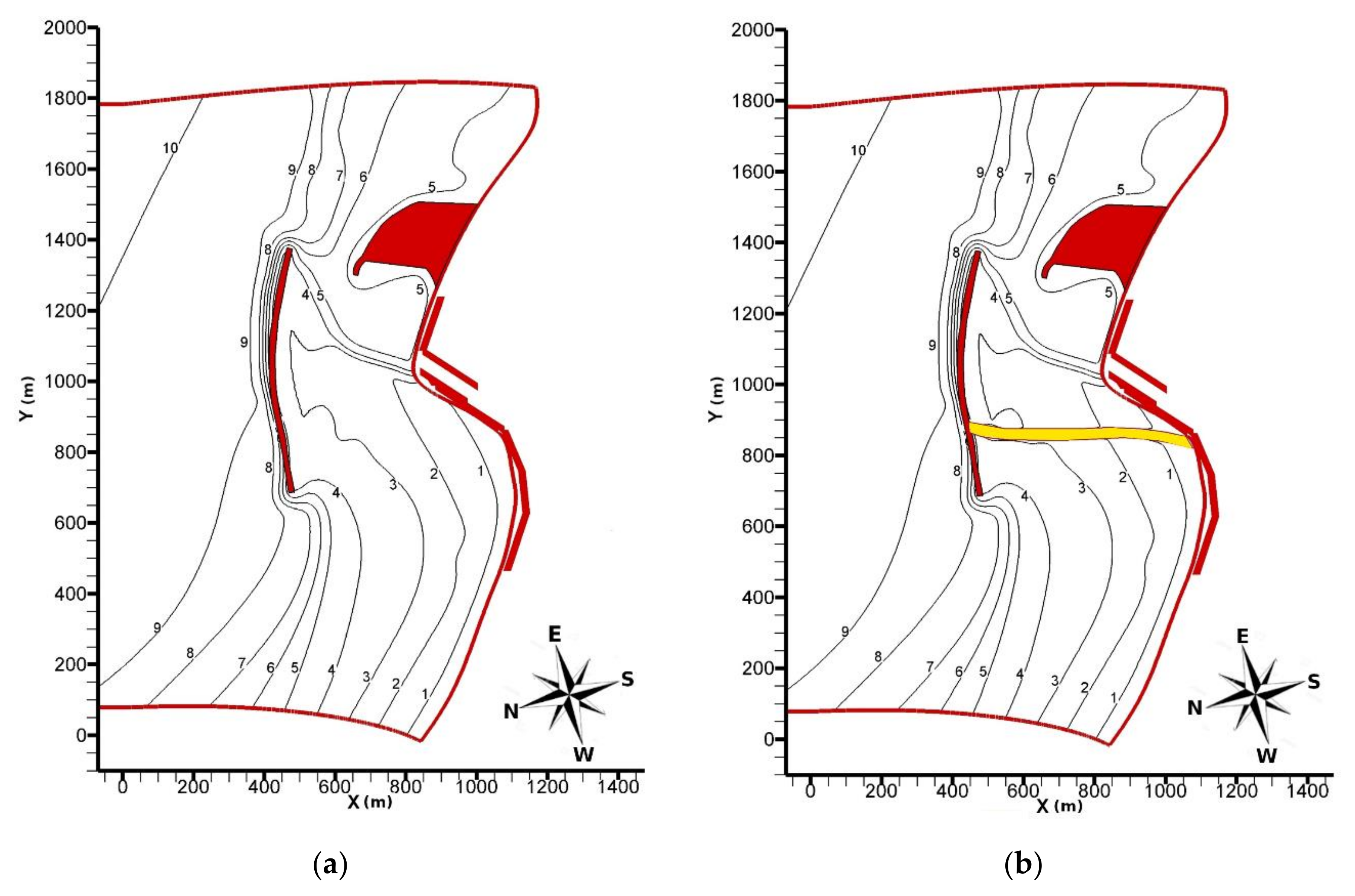
3.1. Configuration 1

Figure 5 shows an instantaneous wave field related to the Configuration 1 whose initial still water depth is shown in Figure 4a. In Figure 5, it is possible to notice that the waves, between $Y=100 \mathrm{m}$ and $Y=700 \mathrm{m}$, at first undergo an increase of the wave height and a reduction of the wavelength (shoaling) and then a decrease of the wave height due to the wave breaking. In particular, we note that the waves, intercepted by the west edge of the detached breakwater, undergo a rotation (diffraction) and, proceeding to the coast, a reduction of the wave height due to the breaking. In the same figure, it is possible to see that, between $Y=700 \mathrm{m}$ and $Y=1500 \mathrm{m}$, the waves are intercepted by the detached breakwater and the Eastern Jetty and undergo a reflection effect due to such structures.

Figure 6 shows a three-dimensional view of the wave field that is shown in Figure 5. In Figure 6, it is possible to notice that the numerical simulation produces wave heights equal to $0.40 \mathrm{m}$ in correspondence of the entrance of the Canal Port: these reduced values of the wave height underline that the detached breakwater improves the navigability conditions at the entrance of the Canal Port.

Figure 7 shows wave- and depth-averaged velocity field produced by the wave field in Figure 5. In Figure 7, it is noted that, in Configuration 1, between $Y=400 \mathrm{m}$ and $Y=1000 \mathrm{m}$, the simulation produces a longshore current that is parallel to the shoreline, characterised by maximum values of the velocity equal to $0.45 \mathrm{m}/\mathrm{s}$. Furthermore, between $Y=1000 \mathrm{m}$ and $Y=1500 \mathrm{m}$, the abovementioned coastal current passes through the detached breakwater and the Eastern Jetty, where it reaches maximum values of the velocity equal to $0.6 \mathrm{m}/\mathrm{s}$.

Figure 8a shows the still water depth (measured from mean water level) produced by the wave field in Figure 5, at the end of the first simulated year in Configuration 1. The still water depth initial conditions used in this numerical simulation are the ones shown in Figure 4a. Compariing Figure 4a and Figure 8a, it is noted a decrease of the still water depth (with consequent sea bottom level increase) in the area between about $X=500 \mathrm{m}$ and $Y=700 \mathrm{m}$ and in the area between $X=450 \mathrm{m}$ and $X=550 \mathrm{m}$, $Y=950 \mathrm{m}$ and $Y=1050 \mathrm{m}$. In this area, at the end of the first simulated year, the $3 \mathrm{m}$ still water depth contour line moves toward the north, with respect to the initial conditions. This comparison also shows a still water depth contour line decrease (with consequent sea bottom level increase) in front of the entrance of the Canal Port. Comparing Figure 4a and Figure 8a shows a decrease of the still water depth (with consequent sea bottom level increase) in the area between $Y=700 \mathrm{m}$ and $Y=1000 \mathrm{m}$, in proximity to the shoreline, where an offshore shift of the $2 \mathrm{m}$ still water depth contour line occurs, from $X=800 \mathrm{m}$ to $X=700 \mathrm{m}$.

Figure 8b presents the still water depth, at the end of the third simulated year in Configuration 1, produced by the wave field in Figure 5. Comparing Figure 8a,b, it is possible to notice a further decrease of the still water depth (with consequent sea bottom level increase) in the area between $X=500 \mathrm{m}$ and between $Y=700 \mathrm{m}$ and $Y=850 \mathrm{m}$. In this area, at the end of the third simulated year, the $3 \mathrm{m}$ still water depth contour line shifts further toward the north. Furthermore, by the same comparison, it is highlighted that there is a further decrease of the still water depth in front of the entrance of the Canal Port. Figure 8b shows that the area (between $X=675 \mathrm{m}$ and $X=750 \mathrm{m}$,$Y=925 \mathrm{m}$ and $Y=1100 \mathrm{m}$) bounded by the $1 \mathrm{m}$ still water depth contour line increases with respect to the one presented in Figure 8a. The same figure also shows that the $2 \mathrm{m}$ still water depth contour line further advances toward the northeast, by reaching $Y=1100 \mathrm{m}$ at the end of the third simulated year. Comparing the results at the end of the first and third simulated years also shows a further decrease of the still water depth (with consequent sea bottom level increase) in the area between $Y=650 \mathrm{m}$ and $Y=800 \mathrm{m}$ and close to the shoreline, where an offshore shift of the $2 \mathrm{m}$ still water depth contour line occurs. The numerical simulations are conducted without taking into account the supply of sediment from Pescara River.

3.2. Configuration 2

Figure 9, Figure 10 and Figure 11 show, respectively, the wave field, the wave- and depth-averaged velocity field and the still water depth, measured from mean water level, related to Configuration 2 characterised by the presence of the submerged breakwater.

In Figure 9, an instantaneous wave field, produced by the same initial conditions used for the simulations of the wave field in Figure 5, is shown. Configuration 2 is characterised by the still water depth shown in Figure 4b. In particular, it can be noticed that the waves, intercepted by the west edge of the detached breakwater, undergo a rotation (diffraction), then proceed towards the shoreline and undergo a reduction of the wave height due to the wave breaking. The same figure shows that the waves diffracted by the west edge of the detached breakwater pass over the submerged breakwater and undergo a reduction of the wave height. In Figure 9, it can be noticed that there are no significant modifications of the wave height in correspondence of the submerged breakwater. This is in marked contrast to the real situation. The reduction of the simulated wave heights is due to the lack of refinement of the computational grid near the submerged breakwater. The fundamental aim of the present study was related to the evaluation, from a global point of view, of the effects on the bottom changes due to the submerged breakwater. The detailed analysis on the wave heights in the area close to the submerged breakwater and on the top of the submerged breakwater is not required for the abovementioned global analysis. The detailed analysis requires the use of small spatial and temporal discretisation steps that increase the computational time very much.

In Figure 10, the wave- and depth-averaged velocity field, produced by the wave field shown in Figure 9, is presented. Figure 10 shows that, in the area between the submerged breakwater and the Eastern Jetty, the maximum value of the velocity is equal to $0.55 \mathrm{m}/\mathrm{s}$. The wave- and depth-averaged velocities on the submerged breakwater are significantly greater than the ones in all the domain and, for this reason, they are not represented in the figure.

Figure 11a shows the still water depth produced by the wave field in Figure 9, at the end of the first simulated year in Configuration 2. The still water depth initial conditions used in this numerical simulation are the ones shown in Figure 4b. Comparing Figure 4b and Figure 11a, it can be noticed that, in the area between the submerged breakwater, the detached breakwater and the entrance of the Canal Port, the still water depth is slightly different from the initial conditions. From the same comparison, it can be also noticed that, in the west area of the submerged breakwater, there is an increase of the sea bottom level. In the area between about $X=700 \mathrm{m}$ and $X=1050 \mathrm{m}$, the $1 \mathrm{m}$, $2 \mathrm{m}$ and $3 \mathrm{m}$ still water depth contour lines advance in the direction of the detached breakwater, with respect to the initial conditions.

In Figure 11b, the still water depth, at the end of the third simulated year, produced by the wave field in Figure 9, is shown. Comparing Figure 11a,b, it can be noticed that, in the area between the submerged breakwater, the detached breakwater and the entrance of the Canal Port, the still water depth is slightly different from the initial conditions. The only contribution of solid material that could modify such sea bottom level is the one coming from the Pescara River. This solid material was not taken into account in the numerical simulation. Comparing Figure 11a,b, it can be noticed that, in the west area of the submerged breakwater, at the end of the third simulated year, there is an accretion of the sea bottom level. In the abovementioned area and between about $X=650 \mathrm{m}$ and $X=1050 \mathrm{m}$ the Figure 11b shows that the $1 \mathrm{m}$, $2 \mathrm{m}$ and $3 \mathrm{m}$ still water depth contour lines advance in the direction of the detached breakwater. There is a significant increase of the seas bottom level in the area between $X=800 \mathrm{m}$ and $\mathrm{X}=950 \mathrm{m}$ and between $\mathrm{Y}=660 \mathrm{m}$ and $\mathrm{Y}=750 \mathrm{m}$, where the still water depth is $1 \mathrm{m}$.

4. Discussion

In this section, we present summary considerations on the results of the numerical simulations relative to the sea bottom changes after three simulated years, either in absence or in presence of the submerged breakwater.

As stated above, the wave motion coming from north direction induces longshore currents coming from northwest direction. The solid material, put into suspension by the wave breaking, is transported by the abovementioned longshore current in the area in front of the entrance of Canal Port. In this area, the energy of the wave motion is consistently damped by the presence of the detached breakwater. Consequently, the solid material silts near the entrance of the Canal Port. The siltation increases the sea bottom levels in front of the entrance of the Canal Port where makes it difficult to navigate.

Figure 12 shows the still water depth contour lines after three simulated years, for Configuration 1. In this figure, the main accretion areas are shown. In the initial configuration (Figure 4a), in front of the entrance of the Canal Port, the still water depth with respect to the mean sea level is about $3 \mathrm{m}$. After three simulated years, in the area coloured in blue in Figure 12, the sea bottom levels increase by about $1 \mathrm{m}$ on average, with a maximum increase of about $2 \mathrm{m}$, and the volume of accumulated sediment is about $\mathrm{25,000}{ \mathrm{m}}^3$. The area in front of the beach, at the northwest of the entrance of the Canal Port, indicated by the red colour in Figure 12, shows an increase of the sea bottom levels by about $1 \mathrm{m}$ on average, with a maximum increase of about $2 \mathrm{m}$, with respect to the initial configuration in Figure 4a. In this area, the volume of accumulated sediment is about $\mathrm{65,000}{ \mathrm{m}}^3$ (after three simulated years). Finally, the area coloured in green in Figure 12, located close to the northwest edge of the detached breakwater (after three simulated years), shows an increase of the sea bottom levels by about $1 \mathrm{m}$, with respect to the initial configuration shown in Figure 4a. In this area, the volume of accumulated sediment is about $\mathrm{20,000}{ \mathrm{m}}^3$.

After the construction of the detached breakwater, periodic measurement campaigns of the still water depth have been carried out by the Italian Ministry of Environment and Protection of Land and Sea [29] in the area between the detached breakwater and the entrance of the Canal Port. In Figure 13, three areas, indicated by A–C, are shown. This classification comes from the fact that, by the abovementioned measurement campaigns, the Italian Ministry of Environment and Protection of Land and Sea carried out an evaluation of the volume of sediment that have accumulated over time in Zone A. The quantification carried out by the measurement campaigns indicates a volume of accumulated sediment of about $\mathrm{40,000}{ \mathrm{m}}^3/\mathrm{year}$.

The volumes of accumulated sediment obtained by the numerical simulations (carried out without the sediment contribution coming from the Pescara River) are: $\mathrm{34,200}{ \mathrm{m}}^3/\mathrm{year}$ in Zone A, $\mathrm{24,500}{ \mathrm{m}}^3/\mathrm{year}$ in Zone B and $\mathrm{22,500} {\mathrm{m}}^3/\mathrm{year}$ in Zone C. The volume of sediment coming from Pescara River is estimated as $\mathrm{10,000}{ \mathrm{m}}^3/\mathrm{year}$ by [29]. By taking into account this contribution, the results obtained by the proposed model are consistent with the measurements carried out by Italian Ministry of the Environment and Protection of Land and Sea [29].

Figure 14 shows still water depth contour lines after three simulated years, for Configuration 2, in the presence of the submerged breakwater. In this figure, the area coloured in green represents the main area that undergoes an increase of the sea bottom level. The volume of sediment accumulated in the area coloured in green, to the northwest of the entrance of the Canal Port, is about $\mathrm{60,000}{ \mathrm{m}}^3$ (after three simulated years).

Figure 15 shows the areas in which the volumes of accumulated sediment are calculated by the numerical simulations. In this configuration, the area previously called A is divided into two sub-areas, A1 and A2, because of the presence of the submerged breakwater. The volumes of accumulated sediment obtained by the numerical simulations (carried out without the sediment contribution coming from the Pescara River) are: $7000{ \mathrm{m}}^3/\mathrm{year}$ in Zone A1, $\mathrm{11,100}{ \mathrm{m}}^3/\mathrm{year}$ in Zone B and $\mathrm{16,100} {\mathrm{m}}^3/\mathrm{year}$ in Zone C. The designed submerged breakwater represents an obstacle to the solid material transport by the longshore currents. This solid material tents to settle in Zone A1, B and C (corresponding to the area bounded by the designed submerged breakwater in the east, by the detached breakwater in the north and by the shoreline in the south).

In absence of the submerged breakwater, the sediment coming from northwest mixes with the sediment coming from the Pescara River and settles in front of the Canal Port. The sediment coming from the northwest is of good quality, while the one coming from the Pescara River is polluted and cannot be used for beach nourishment. The presence of the submerged breakwater blocks the pollution-free sediment that can be used for beach nourishment. Furthermore, as stated above, the submerged breakwater, blocking the solid material coming from northwest, significantly limits the increase of the sea bottom level in front of the entrance of the Canal Port and, consequently, makes it possible to maintain good navigability conditions.

5. Conclusions

The real case study of Pescara Harbour (Italy) was investigated by means of a numerical bottom-change simulation model, composed by a hydrodynamic sub-model and a morphodynamic sub-model. In particular, the effects of the introduction of a designed submerged breakwater in the existing context were studied in terms of morphodynamic alterations. The used hydrodynamic model is based on an integral form of the fully nonlinear Boussinesq equations, while the proposed morphodynamic model is based on a quasi-three-dimensional approach. It was demonstrated (by numerical simulations) that the detached breakwater, built to reduce the navigation risks at the entrance of the Canal Port, damps the energy of the wave motion and causes the siltation of the solid materials, transported by the longshore current coming from northwest, in front of the harbour entrance. From the numerical investigation carried out, it can be seen that the designed submerged barrier substantially modifies the hydrodynamic field and the morphodynamic evolution of the zone near Pescara Harbour. In particular, the ability of the designed submerged breakwater, located orthogonally to the longshore current, to intercept the aforementioned solid material and to significantly reduce the accretion of the bottom in the area in front of the entrance of the Canal Port entrance, was verified.

References

1. Mortlock, R.T.; Goodwin, I.D.; McAneney, J.K.; Roche, K. The June 2016 Australian East coast low: Importance of wave direction for coastal erosion assessment. Water 2017, 9, 121. [Google Scholar] [CrossRef]
2. Nguyen, C.Q.; Goodwin, I.D.; Mortlock, T.R.; Gallop, S.L. The influence of wind on hydrodynamic processes in Robbins Passage, Tasmania, Australia. J. Coast. Res. 2018, 85, 141–145. [Google Scholar] [CrossRef]
3. Cannata, G.; Gallerano, F.; Palleschi, F.; Petrelli, C.; Barsi, L. Three-dimensional numerical simulation of the velocity fields induced by submerged breakwaters. Int. J. Mech. 2019, 13, 1–14. [Google Scholar]
4. Cannata, G.; Petrelli, C.; Barsi, L.; Gallerano, F. Numerical integration of the contravariant integral form of the Navier-Stokes equations in time-dependent curvilinear coordinate systems for three-dimensional free surface flows. Continuum Mech. Therm. 2019, 31, 491–519. [Google Scholar] [CrossRef] [Green Version]
5. Losada, I.J.; Lara, J.L.; del Jesus, M. Modeling the interaction of water waves with porous coastal structures. J. Waterw. Port. Coast. Ocean. Eng. 2016, 142, 1–18. [Google Scholar] [CrossRef]
6. Losada, I.J.; Lara, J.L. Chapter 32: Three-dimensional modeling of wave interaction with coastal structures using Navier-Stokes Equations. In Handbook of Coastal Ocean Engineering; Young, C.K., Ed.; California State University: Los Angeles, CA, USA, 2018; pp. 919–943. [Google Scholar]
7. Cannata, G.; Lasaponara, F.; Gallerano, F. Non-linear Shallow Water Equations numerical integration on curvilinear boundary-conforming grids. WSEAS Trans. Fluid Mech. 2015, 10, 13–55. [Google Scholar]
8. Postacchini, M.; Ludeno, G. Combining Numerical Simulations and Normalized Scalar Product Strategy: A New Tool for Predicting Beach Inundation. J. Mar. Sci. Eng. 2019, 7, 325. [Google Scholar] [CrossRef] [Green Version]
9. Ikha, M.; Atras, M.F.; Sembiring, L.; Nugroho, M.A.; Roi Solomon, B.L.; Roque, M.P. Wave Transmission by Rectangular Submerged Breakwaters. J. Mar. Sci. Eng. 2020, 8, 56–74. [Google Scholar]
10. Kian, R.; Velioglu, D.; Yalciner, A.C.; Zaytsev, A. Effects of Harbor Shape on the Induced Sedimentation; L-Type Basin. J. Mar. Sci. Eng. 2016, 4, 55. [Google Scholar] [CrossRef]
11. Lo Re, C.; Manno, G.; Ciraolo, G. Tsunami propagation and flooding in Sicilian Coastal Areas by means of a weakly dispersive Boussinesq model. Water 2020, 12, 1448. [Google Scholar] [CrossRef]
12. Liu, W.; Ning, Y.; Zhang, Y.; Zhang, J. Shock-capturing Boussinesq modelling of broken wave characteristics near a vertical seawall. Water 2018, 10, 1876. [Google Scholar] [CrossRef] [Green Version]
13. Gallerano, F.; Cannata, G.; Villani, M. An integral contravariant formulation of the fully non-linear Boussinesq equations. Coast. Eng. 2014, 83, 119–136. [Google Scholar] [CrossRef] [Green Version]
14. Petti, M.; Bosa, S.; Pascolo, S. Lagoon sediment dynamics: A coupled model to study a medium-term silting of tidal channels. Water 2018, 10, 569. [Google Scholar] [CrossRef] [Green Version]
15. Shi, F.; Kirby, J.T.; Harris, J.C.; Geiman, J.D.; Grilli, S.T. A high-order adaptive time stepping TVD solver for Boussinesq modelling of breaking waves and coastal inundation. Ocean. Model. 2012, 43–44, 35–51. [Google Scholar] [CrossRef]
16. Gallerano, F.; Cannata, G.; Scarpone, S. Bottom changes in coastal areas with complex shorelines. Eng. Appl. Comput. Fluid Mech. 2017, 11, 396–416. [Google Scholar] [CrossRef]
17. Tonelli, M.; Petti, M. Finite volume scheme for the solution of 2D extended Boussinesq equations in the surf zone. Ocean. Eng. 2010, 37, 567–582. [Google Scholar] [CrossRef]
18. Tonelli, G.; Petti, M. Shock-capturing Boussinesq model for irregular wave propagation. Coast. Eng. 2012, 61, 8–19. [Google Scholar] [CrossRef]
19. Lynett, P.J. Nearshore wave modelling with high-order Boussinesq-type equations. J. Waterw. Port. Coast. Ocean. Eng. 2006, 132, 348–357. [Google Scholar] [CrossRef] [Green Version]
20. Wei, G.; Kirby, J.T.; Grilli, S.T.; Subramanya, R. A fully non-linear Boussinesq model for surface waves. Part 1: Highly nonlinear unsteady waves. J. Fluid Mech. 1995, 294, 71–92. [Google Scholar] [CrossRef]
21. Chen, Q.; Kirby, J.T.; Dalrympe, R.A.; Shi, F.; Thornton, E.B. Boussinesq modeling of longshore currents. J. Geophys. Res. 2003, 108, 26–28. [Google Scholar] [CrossRef]
22. Chen, Q. Fully non-linear Boussinesq-type equations for waves and currents over porous beds. J. Fluid Mech. 2006, 132, 220–230. [Google Scholar]
23. Drønen, N.; Deigaard, R. Quasi-three-dimensional modelling of the morphology of longshore bars. Coast. Eng. 2007, 54, 197–215. [Google Scholar] [CrossRef]
24. Kim, N.H.; An, S.H. Numerical computation of the nearshore current considering wave-current interactions a Gangjeong coastal area, Jeju Island, Korea. Eng. Appl. Comp. Fluid Mech. 2011, 5, 430–444. [Google Scholar] [CrossRef] [Green Version]
25. Thompson, J.; Warsi, Z.U.A.; Mastin, C.W. Numerical Grid Generation; Elsevier North-Holland: New York, NY, USA, 1985. [Google Scholar]
26. Deigaard, R.; Fredsøe, J.; Hedegaard, I.B. Suspended sediment tin the surf zone. J. Waterw. Port. Coast. Ocean. Eng. 1986, 112, 115–128. [Google Scholar] [CrossRef]
27. Rakha, K.A.; Deigaard, R.; Brøker, I. A phase-resolving cross shore sediment transport model for beach profile evolution. Coast. Eng. 1997, 31, 231–261. [Google Scholar] [CrossRef]
28. Italian Ministry of the Environment and Protection of Land and Sea “Studio Meteomarino—Piano Regolatore Portuale del Porto di Pescara”, 2008, 14. Available online: www.va.minambiente.it (accessed on 1 December 2008).
29. Italian Ministry of the Environment and Protection of Land and Sea “Studio Morfologico—Piano Regolatore Portuale del Porto di Pescara”, 2008, 22–24. Available online: www.va.minambiente.it (accessed on 1 December 2008).
Figure 1. Map of Italy in which the study site of the Pescara Harbour is indicated by a red point.
Jmse 08 00487 g001
Figure 2. Satellite view of the Pescara Harbour coastal area.
Jmse 08 00487 g002
Figure 3. Schematic representation of a plan view of Pescara Harbour and near region. The blue and orange arrows indicate respectively the primary and secondary sector incoming waves. The green and red arrows indicate the longshore currents produced respectively by the primary and secondary sector incoming waves.
Jmse 08 00487 g003
Figure 4. Plan view of Pescara Harbour and the still water depth measured from mean water level: (a) Configuration 1; and (b) Configuration 2.
Jmse 08 00487 g004
Figure 5. Instantaneous wave field. Present sea bottom level. Configuration 1.
Jmse 08 00487 g005
Figure 6. The instantaneous wave field. Present sea bottom level. Configuration 1.
Jmse 08 00487 g006
Figure 7. Calculated wave- and depth-averaged velocity field (one vector out of every four). Present sea bottom level. Configuration 1.
Jmse 08 00487 g007
Figure 8. Configuration 1. Still water depth, measured from mean water level, after: (a) one year; and (b) three years.
Jmse 08 00487 g008
Figure 9. Instantaneous wave field. Present sea bottom level. Configuration 2.
Jmse 08 00487 g009
Figure 10. Calculated wave and depth averaged velocity field (one vector out of every four). Present sea bottom level. Configuration 2.
Jmse 08 00487 g010
Figure 11. Configuration 2. Still water depth, measured from mean water level, after: (a) one year; and (b) three years.
Jmse 08 00487 g011
Figure 12. Configuration 1. Accretion areas after three simulated years.
Jmse 08 00487 g012
Figure 13. Zones partition for the evaluation of the volume of settled sediment. Configuration 1.
Jmse 08 00487 g013
Figure 14. Configuration 2. Accretion areas after three simulated year.
Jmse 08 00487 g014
Figure 15. Zones partition for the evaluation of the volume of sedimented materials. Configuration 2.
Jmse 08 00487 g015