3.1. Research Method
This study aimed to determine the primary cargo types of supply chains, according to cargo type in the adjacent areas around the target port, that have a high influence on fine dust concentrations over one month. Based on the advanced research in 2.2, it was found that the concentrations of
,
, and
are highly affected by meteorological factors (wind direction, temperature, humidity, and atmospheric pressure) and are seasonal in response to patterns of atmospheric circulations. This method was carried out in 4 steps. In step 1, a correlation analysis was conducted between the bulk cargo throughput primarily handled in Gamcheon Port, and the PM concentrations were extracted by seasonal factors through the X11 method from the time series data of PM (
,
,
) over time. The X11 method, which is a filter based method of seasonal adjustment, was invented by the US Census Bureau and Statistics Canada. X11 is used to estimate and remove seasonal and irregular components that happen repeatedly in a regular pattern in time series data. It is also used to provide a more accurate result through time series analysis [
16].
Equation (1). Pearson Correlation Coefficient Equation:
The Pearson Correlation Coefficient (described as in Equation (1)) is used to ascertain the level and direction of relations between two coefficients showing a linear relation in a normal distribution [
17]. The variables of Equation (1) are as follows; x—value of independent variables,
—mean of independent variables, y—value of dependent variables,
—mean of dependent variables, and n—pairs of numbers x and y. However, the causality relationship cannot be proven by correlation only because correlation is only one of the premises. In other words, correlation is a necessary condition for causality relationships. In step 2, stationarity tests was conducted on the time series data derived from step 1 using the Augmented Dickey–Fuller (ADF) and KPSS ((Kwiatkowski–Phillips–Schmidt–Shin) tests, which are complementary to each other. As the time series data lacks stability, there is a risk that a false statistical result could emerge.
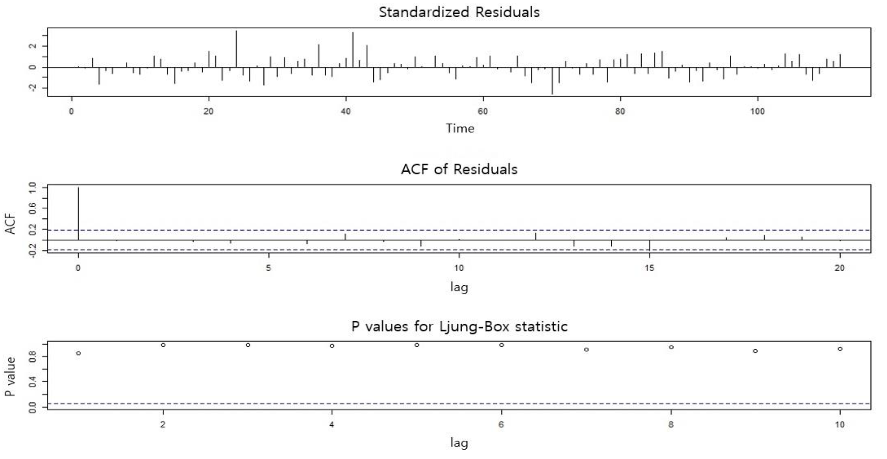
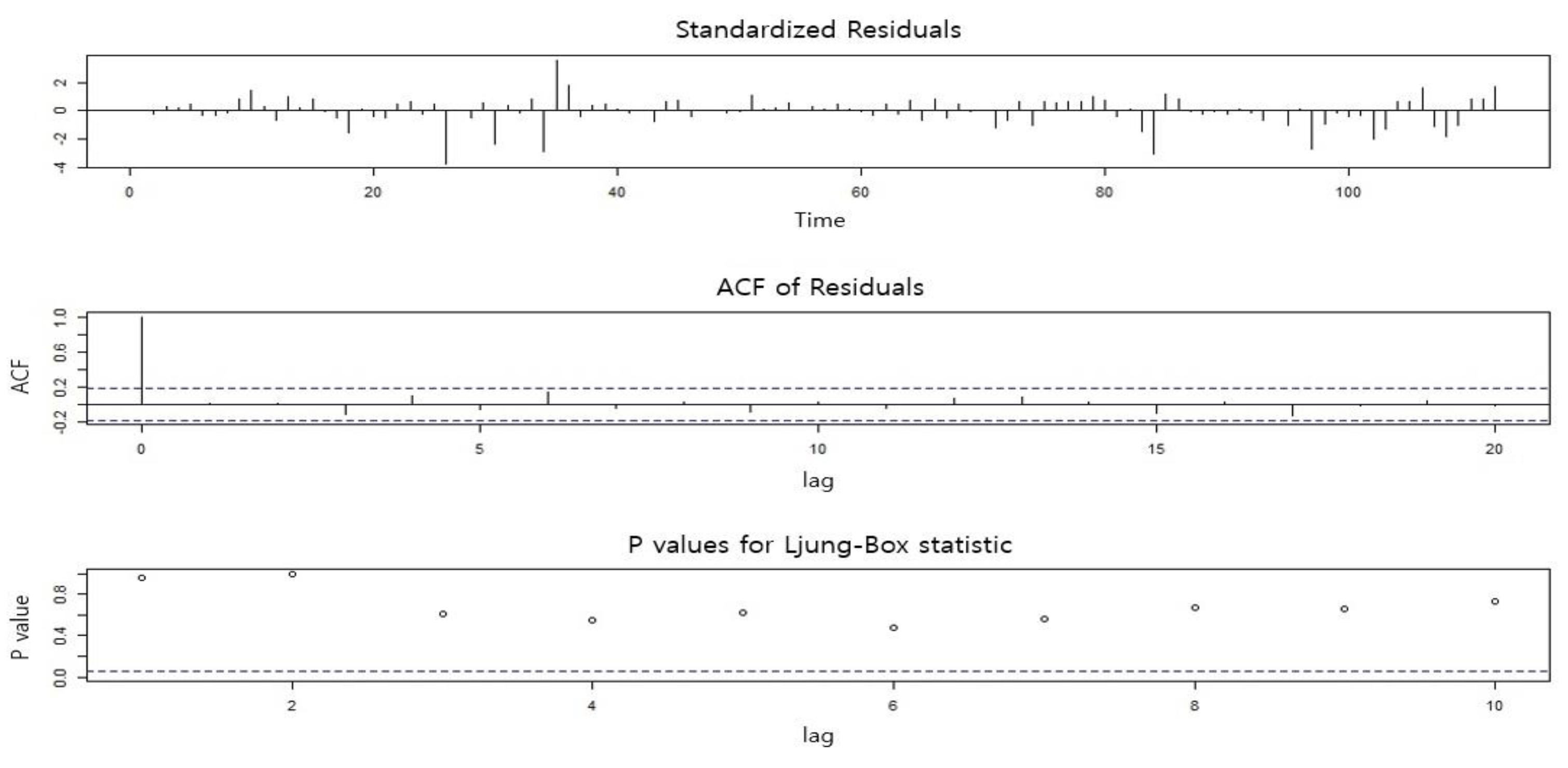
In step 3, ARIMA models were fitted for the derived independent variables. The output time series data were constructed by applying the operator of independent variables, the ARIMA operator, to the ARIMA models of the dependent variables. Time series models are classified into autoregressive (AR), moving average (MA), autoregressive moving average (ARMA), and autoregressive integrated moving average (ARIMA) models. Residuals (), which are components of the models, signify the estimated value representing the difference between the real and estimated values from the fitted models. White noise is defined as a time series without autocorrelation between the residuals ().
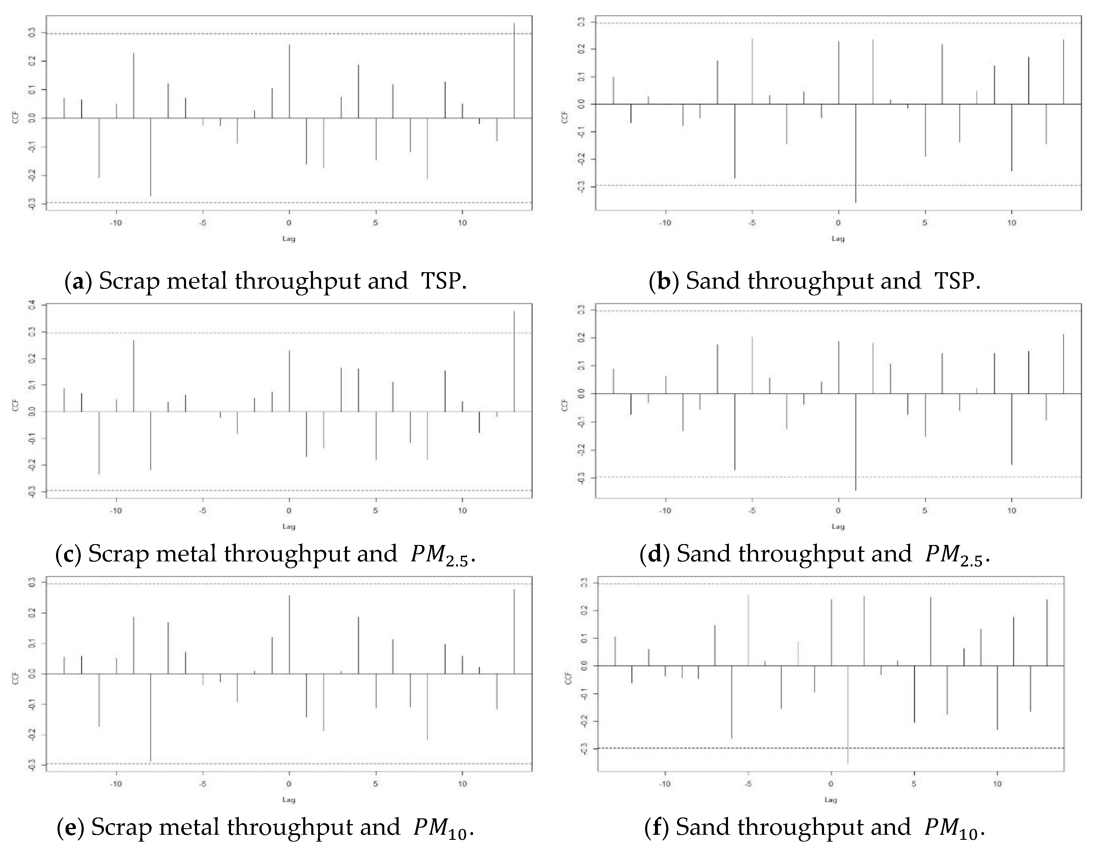
In step 4, the time series data were pre-whitened and then assessed to ensure they represent white noise via a cross-correlation graph. Then, a Granger causality test was conducted to determine whether statistical causality is present in the time series data of the primary cargo types that emit fine dust. Due to the autocorrelation in time series data, the process to remove autocorrelation in the data before ascertaining cross-correlation could lead to false cross-correlation, which is called pre-whitening [
18]. The pre-whitening procedure in the ARIMA model proceeds by choosing a proper model, selecting a proper parameter value based on the estimated function, and then evaluating the model.
Equation (2), cross-correlation coefficient:
The correlation between consecutive observed values in a time series classified by the range of time difference is known as cross-correlation; the cross-correlation coefficient is described by Equation (2), which indicates the correlation between two time series’ estimated values, and , classified by the time difference unit, k. The construction of Equation (2) is the same as Equation (1), except for the time difference, k. To test the Granger causality, it is necessary to ensure that the time series data indicate white noise by cross-correlation (Equation (2)). The time difference, , is added to the equation to draw the coefficient of variables X and Y, whose ordering relationship is determined by k’s negative or positive value that brings to its maximum. In other words, if k < 0, X is preceded by Y; if K = 0, X and Y are together; and if k > 0, X is followed by Y. That is, can be calculated by with the time difference of k.
Equation (3), Granger causality:
The Granger causality test is a technique used to define the causality of dependent (Y) and independent variables (X) in the linear regression model. When the past time series data (X) and (Y) are predicted linearly from two time series data, there is said to be causality if the resulting value, predicted linearly with only Y, is significant (and vice versa) in the formula described in Equation (3) [
19]. In other words, if the condition of
is satisfied under the assumption of uncorrelated white noise for the error terms (
,
), the variable X is determined to be causal for variable Y, and vice versa. In the formula,
and
represent the intercept coefficients, and
,
,
, and
represent the slope coefficients. The Granger causality test determines whether the variable affects not only the time difference k but also its lag. This study derives the type of cargo emitting fine dust based on a correlation analysis between the bulk cargo primarily handled by Gamcheon Port and fine dust concentrations and also investigates the causality between the derived cargo types and fine dust concentrations.
3.2. Target Port
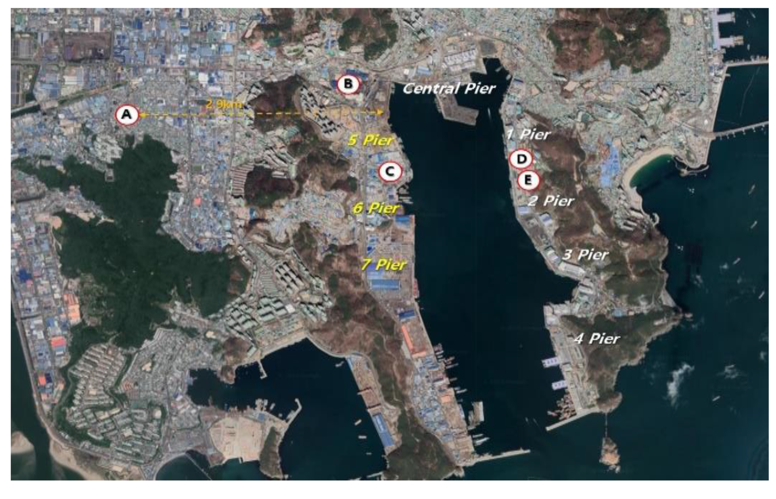
The target port in this study is Gamcheon Port in Busan, South Korea. The port’s primary bulk cargo, including scrap metal, sand and cement, are chiefly processed in the west ports from pier 5 to 7, as shown in
Figure 4. In total, 103,647 tons of scrap metal were processed in 2016, 118,119 tons in 2017, and 78,552 tons in 2018, representing a ratio of 46.5% in 2016, 78% in 2017, and 86.5% in 2018 compared to the amount of scrap metal managed in the ports that comprise the Port of Busan. A total of 683,328 tons of sand cargo was processed in 2016, 865,454 tons in 2017, and 562,648 tons in 2018, with a ratio of 34.1% in 2016, 54.1% in 2017, and 51.1% in 2018 compared to the amount of sand processed in the other ports of the Port of Busan. Furthermore, for cement cargo, 1,774,236 tons, 2,201,750 tons, and 1,909,674 tons were processed from 2016 to 2018, respectively, and approximately 100% of such cargo imported to the Port of Busan were handled in Gamcheon Port.
Figure 4 illustrates the distribution of factories near Gamcheon Port. The supply chains located in Gamcheon Port and its adjacent areas are YK Steel (B), which handles scrap metal; Ssangyong Cement Industrial (C) and Sampyo Cement (D), which handle sand and cement cargo; and Tongyang Aggregate (E), which manages sand cargo. The concentration data used in this research for
,
, and
were measured from the air quality observatory (A) located at a radius of 2.9 km from the west port of Gamcheon Port.
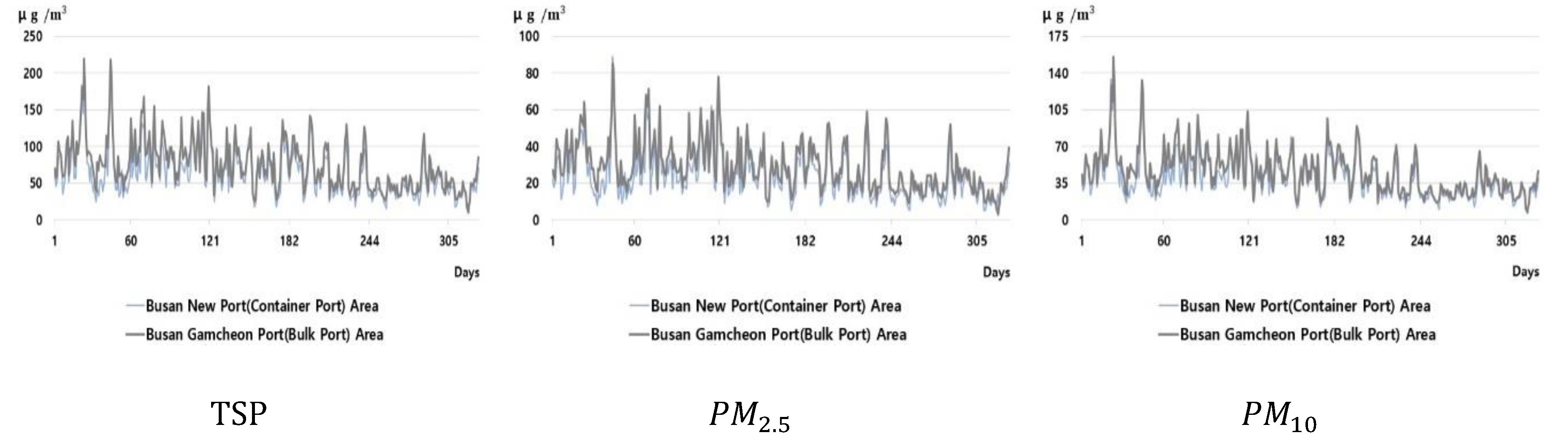
Figure 5 provides graphs comparing the concentration data of
,
, and
collected by an air quality observatory located in Busan New Port (container port) and Gamcheon Port (bulk port), from 7 November 2018, when
began to be measured at Busan New Port, to 30 September 2019 (328 days in total). Compared to Busan New Port, higher concentrations of
were found for 298 days,
for 307 days, and
for 301 days in Gamcheon Port. Thus, the industrial activities derived from bulk ports are responsible for air pollution in the adjacent areas. Therefore, PM and oxide dust are produced in a relatively large volume compared to container ports due to their dusty nature and processing of heavy cargo.


