2.2.1. Model Description
In this work, OpenFOAM v6 [
42] was applied and validated, or more specifically interFoam, a solver of the RANS equations, where the advection and sharpness of the water–air interface are handled by an algebraic VOF method [
43] based on the multidimensional universal limiter with explicit solution (MULES) [
44,
45,
46]. InterFoam with MULES has already been successfully applied for wave propagation [
45], wave breaking [
20,
47,
48,
49,
50], wave run-up [
20,
50], wave overtopping [
51,
52], and bore impact on a vertical wall [
26].
Several open source contributions of boundary conditions for wave generation and absorption exist for interFoam, of which the main developments are IHFOAM [
53], olaFlow [
54], and waves2Foam [
55]. In the present study, olaFlow was chosen, which was found to be the most computational efficient [
53,
56,
57] and feature complete package at the time of the simulations presented in this paper.
The turbulence is modelled by the
k-
ω SST turbulence closure model [
58], which has been shown to be one of the most proficient in modelling wave breaking [
47]. Two-equation turbulence closure models are known to cause over-predicted turbulence levels beneath computed surface waves, leading to unphysical wave decay for wave propagation over constant water depth and long distance [
49,
59,
60]. Turbulence modelling was therefore stabilized in nearly potential flow regions by Larsen and Fuhrman [
49], with their default parameter values [
61]. Hereafter, the OpenFOAM numerical model as presented here is simply referred to as OF.
2.2.2. Computational Domain and Mesh
Wave breaking is an inherently three-dimensional (3D) process due to the formation of 3D vortices extending obliquely downward in the inner surf zone [
62]. Even so, many examples exist where the wave kinematics during wave breaking could be approximated well by vertical two-dimensional (2DV) RANS modelling [
8,
19,
47,
48,
49,
50,
63,
64]. To reduce the computational time as much as possible, OF is therefore applied in a 2DV configuration (i.e., cross-shore section of the wave flume).
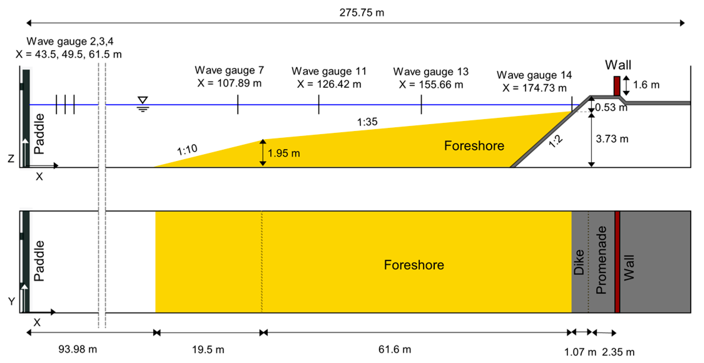
The OF model domain (
Figure 3) starts at the wave paddle zero position (
x = 0.00 m) and ends on top of the vertical wall (
x = 178.80 m). The bottom boundary is at its lowest point (
z = 0.00 m) along the flume bottom between the wave paddle and the foreshore toe, and extends up to z = 7.20 m, well above the maximum measured surface elevations along the flume. The bottom is further defined by the measured foreshore and dike geometry as described in
Section 2.1. The vertical wall is included up to its height of 1.60 m including the top which was given a slight inclination towards the model boundary to allow overtopped water (limited to mainly spray in this case) to exit the model domain.
The computational domain is discretised into a structured grid. To optimise the computational time, a variable grid resolution is applied, where a higher resolution is defined only where it is necessary. This is mostly the areas of the model domain where the water-air interface is expected to pass [
46,
56]. The expected location of the free surface along the flume during the entire test was estimated first by a fast preliminary one-layer depth-averaged SWASH calculation (not shown: see [
65] for the SWASH model setup description). The minimum and maximum
η along the flume and over the complete test duration were obtained from the SWASH model result to define areas in which mesh refinement should be done. These locations are delineated by the dotted lines in
Figure 3, defining several areas around the still water level (
SWL). In front of the wave paddle, the refinement area is slightly higher to accommodate the stabilisation of the newly generated waves, after which the refinement zone can decrease in height when the waves have fully developed. Then, the refinement area is increased in height again to allow room for wave shoaling and incipient wave breaking on the foreshore. The upper limit can subsequently be lowered again due to wave breaking, but the lower limit is extended to include the bottom boundary. This is done to properly resolve the entrained air pockets that have been shown to travel towards the bottom during the breaking process in the inner surf zone [
66]. The height of the refinement zone on the dike was defined based on the maximum measured water level in the experiment by the WLDM’s on the promenade and extended to the upper model boundary along the vertical wall to resolve the run-up and splashing against the vertical wall.
In terms of the grid cell size in these refinement zones, about 20 cells are typically recommended over the wave height
H of a regular wave (i.e.,
H/Δ
z = 20, with Δ
z being the vertical cell size) [
46,
57]. Applied to the wave heights of the primary wave components of the bichromatic wave in
Table 1, a minimal vertical cell size of Δ
z = 0.045 m to 0.043 m is obtained. Smaller wave heights in the bichromatic wave group are less resolved with this choice, but this is deemed acceptable because of their relatively low steepness. A value of Δ
z = 0.045 m was chosen, because the water depth at the wave paddle
ho is divisible by it (i.e.,
ho/Δ
z = 4.14/0.045 = 92), meaning that the
SWL can lie perfectly along cell boundaries, or in other words, α-values between 0 and 1 are thereby minimised at the start of the simulation, which simplifies the initialisation of the
SWL and is beneficial for an effectively still
SWL at the start of the simulation.
The mesh maintains an aspect ratio Δ
x/Δ
z of 1 (with Δ
x being the horizontal cell size) throughout the entire computational domain, which has been shown necessary for accuracy [
46,
55,
66] and numerical stability in this study. One exception is a higher aspect ratio along the bottom and wall, where layers were locally added to the mesh to resolve the boundary layer. Six layers were added over the vertical cell size along those boundaries, with a growth rate of 1.2, leading to a maximum aspect ratio of 18.
Outside the refinement zones, in the air and water phases, the mesh can be coarser [
46,
57]. The structured mesh was given a base grid resolution of 0.18 m. This base resolution is multiplied by a refinement ratio
r, here defined as:
in which
β signifies the refinement level. Each refinement level effectively refines every cell into four new cells. The applied refinement levels are provided for each mesh subdomain in
Figure 3. For the air in the model domain, the base resolution was assumed (
β = 0), except for a small area over the dike (
β = 1). In the water phase, refinement level 1 was assumed (Δ
x = Δ
z = 0.09 m) and was further refined in the zone of the surface elevation up to the dike toe (level 2 or Δ
x = Δ
z = 0.045 m). Close to the inlet boundary, however, a lower refinement level was necessary for numerical stability (
β = 1) over a very short distance (0 m <
x < 0.50 m) where locally high water velocities (i.e., low Courant numbers and low time steps) at the interface can occur due to the wave generation. On the dike up to the wall, the mesh was refined even more (level 3 or Δ
x = Δ
z = 0.0225 m) to resolve thin layer flows, the complex flows of bore interactions, and impacts on the vertical wall. In addition, a refinement level 3 was necessary to resolve the experimental pressure sensor locations along the vertical wall.
The mesh was generated by applying the
cartesian2DMesh algorithm of cfMesh [
67], which resulted in a mesh with 318,381 cells, for the refinement levels indicated in
Figure 3.
The adaptive time stepping is controlled by a predefined maximum Courant number
maxCo (
Co = ∆
t |
U|/∆
X, where ∆
t is the time step, |
U| is the magnitude of the velocity through that cell, and ∆
X is the cell size in the direction of the velocity [
68]) and a maximum Courant number in the interface cells
maxAlphaCo. Generally
maxCo =
maxAlphaCo is chosen, as well as in this paper. Larsen et al. [
45] have shown that a relatively low
maxCo (~0.05) is necessary to obtain a stable wave profile over more than five wave periods’ propagation duration. Here, however, a
maxCo of 0.25 is used to balance the accuracy and computational costs. Since the primary waves of the bichromatic wave group only propagate over about three wave lengths up to the mean breaking point location (
xb = ~120 m), this is considered an acceptable assumption. Both the refinement level in the refinement zones around the surface elevation zones (
βsez) and the
maxCo were verified in a convergence analysis (
Appendix A).
2.2.3. Boundary Conditions
Since the model domain represents a 2DV simulation, no solution is necessary in the
y-direction, and the lateral boundaries of numerical wave flume were assigned an “empty” boundary condition. Non-empty boundary conditions were defined for the remaining boundaries in the
xz-plane (
Figure 3).
The bichromatic waves from
Table 1 were generated at the inlet by applying a Dirichlet-type boundary condition: the experimental wave paddle velocity was imposed. The paddle displacement time series is used by olaFlow to calculate the wave paddle velocity by a first-order forward derivative [
69]. Since the reflection in the numerical wave flume is expected to behave close to, but not exactly the same as in the experiment, the theoretical paddle displacement without ARC was selected and the AWA by olaFlow was activated instead. In addition to the paddle displacement, the surface elevation at the wave paddle is provided, which allows olaFlow to trigger the AWA with fewer assumptions [
69]. The AWA implementation in olaFlow is most effective for shallow water waves. The primary components of the bichromatic wave group are intermediate waves for the water depth at the wave paddle, but their reflection is expected to be low, since most of their wave energy dissipates over the foreshore in the surf zone. However, reflected free long (infragravity) waves are expected to be non-negligible (
Section 3.2). They are shallow water waves and are by definition absorbed well by the AWA system in olaFlow, preventing their re-reflection and therefore replicating the behaviour of the ARC in the experiment.
Both the bottom and wall boundaries are fixed boundaries, including the sandy foreshore (
Section 2.1), along which the velocity vector field
U has a Dirichlet-type boundary condition (
U = (0, 0, 0) m/s), while the pressure
p and α are given a Neumann boundary condition. Along the foreshore, dike and wall, no-slip boundary conditions are assumed and a continuous scalable wall function based on Spalding’s law [
70] is implemented. The six boundary layers that were previously added in the mesh along these no-slip fixed boundaries make sure that the scalable wall function criterion for the dimensionless wall distance
z+ (i.e., 1 <
z+ < 300) is complied with. For the remaining boundary conditions, initial conditions, and solver settings, the same settings were chosen as those reported by Devolder et al. [
48].
The OF simulations were run in parallel on a 24-core Intel Xeon E5-2680 @ 2500 MHz computer with 128 GB of RAM. The scotch decomposition algorithm was used to divide the mesh into equal amounts of cells for each processor, while minimising the number of processor boundaries [
42]. The cells along the inlet patch were forced onto the same processor, which benefits the computational efficiency. In this setup, the simulation required a CPU time of about 85 h.
2.2.4. Data Sampling and Processing
The same data were sampled in OF at the same cross-shore locations as in the experiment (
Section 2.1). Applying the same sampling frequency of 1000 Hz in OF, however, would increase the calculation time to unpractical levels because it affects the time stepping. Instead, a sampling frequency of 80 Hz was maintained throughout, which is a compromise between the temporal resolution of the output data and the calculation time.
To obtain
η in OF, α was recorded at a fixed interval over a vertical line at each wave gauge location. In post-processing,
η was then obtained by vertical integration of α, thereby excluding air inclusions produced in the surf zone, but taking into account all water volumes (i.e., even air-borne water, e.g., in case of plunging waves, spray). This corresponds best to how
η in the experiment was measured: resistive wave gauges give a response proportional to the wire wet length [
71], thereby similarly excluding air pockets. However, it is acknowledged that some uncertainty remains regarding how resistive type wave gauges measure the free surface in the presence of air–water mixtures along the gauge. This could lead to discrepancies in the numerical–experimental model comparisons in the surf zone and on top of the promenade [
72].
The resulting numerical time series were filtered in the same way as the experimental data (
Section 2.1) and were synchronised to the experimental time reference. The synchronisation was done based on the
η time series at the three most offshore located wave gauges (i.e., WG02–03–04) by means of a cross-correlation. The obtained numerical–experimental time lags for each of these WG locations were subsequently averaged and rounded to the nearest multiple of the time series time step. This time lag was then used to synchronise all numerical time series to the experimental time reference. This makes sure that numerical errors (such as phase lag), which are important for model validation, were retained.
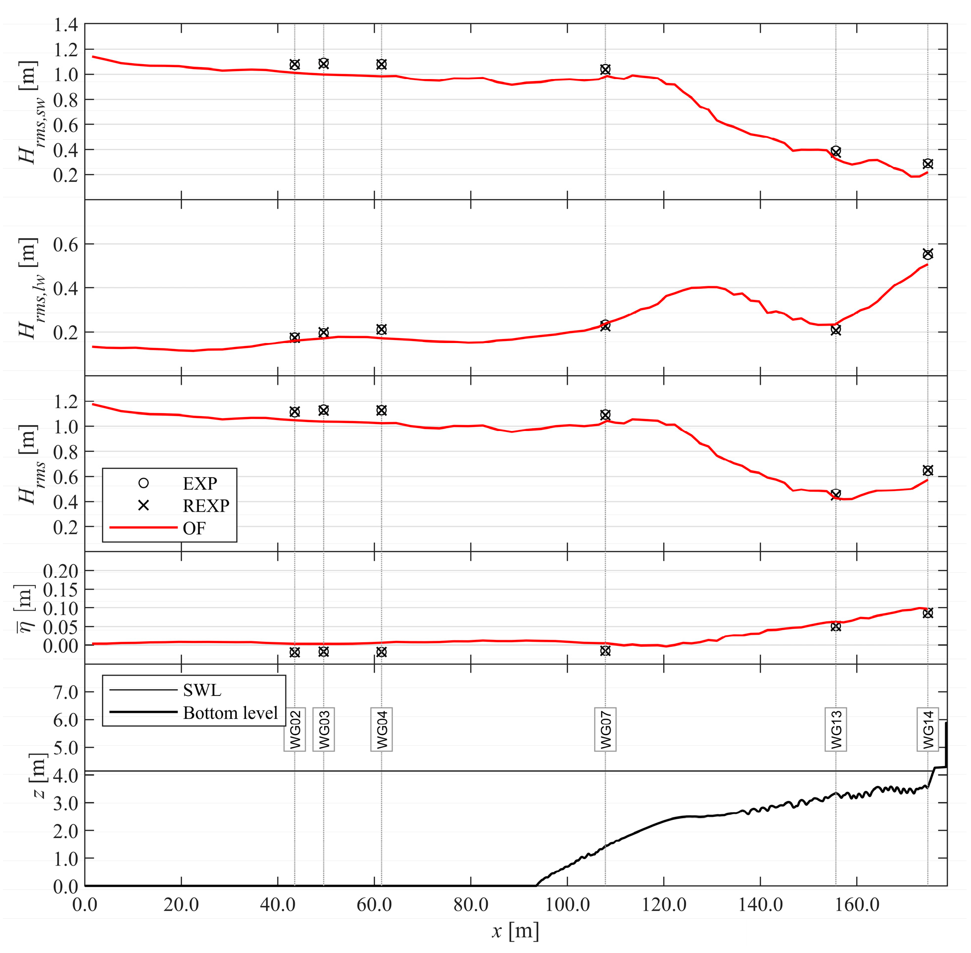
Furthermore, to investigate the model performance for the SW and LW components separately, the η time series were separated into ηSW and ηLW by applying a 3rd-order Butterworth high- and low-pass filter, respectively. A separation frequency of 0.09 Hz was employed, which is in between the bound long wave frequency (f1–f2 = 0.035 Hz) and the lowest frequency of the primary wave components (f2 = 0.155 Hz).

 ,
, 


