Inversion of the Thickness of Crude Oil Film Based on an OG-CNN Model

Abstract

In recent years, marine oil spill accidents have occurred frequently, seriously endangering marine ecological security. It is highly important to protect the marine ecological environment by carrying out research on the estimation of sea oil spills based on remote sensing technology. In this paper, we combine deep learning with remote sensing technology and propose an oil thickness inversion generative adversarial and convolutional neural network (OG-CNN) model for oil spill emergency monitoring. The model consists of a self-expanding module for the oil film spectral feature data and an oil film thickness inversion module. The feature data self-expanding module can automatically select spectral feature intervals with good spectral separability based on the measured spectral data and then expand the number of samples using a generative adversarial network (GAN) to enhance the generalization of the model. The oil film thickness inversion module is based on a one-dimensional convolutional neural network (1D-CNN). It extracts the characteristics of the spectral feature data of oil film with different thicknesses, and then accurately inverts the oil film’s absolute thickness. In this study, emulsification was not a factor considered, the results show that the absolute oil thickness inversion accuracy of the OG-CNN model proposed in this paper can reach 98.12%, the coefficient of determination can reach 0.987, and the mean deviation remains within ±0.06% under controlled experimental conditions. In the model stability test, the model maintains relatively stable inversion results under the interference of random Gaussian noise. The accuracy of the oil film thickness inversion result remains above 96%, the coefficient of determination can reach 0.973, and the mean deviation is controlled within ±0.6%, which indicates excellent robustness.

1. Introduction

Marine oil spill disasters seriously affect the marine ecological environment and resources [1,2]. Sea oil spill is an important indicator for assessing the threat of marine oil spill accidents and determining the level of oil spill accidents, and is also an important basis for determining pollution compensation liability. At the same time, it plays an important role in emergency on-site oil spill disposal and scientific decision-making. Accurately obtaining the oil film thickness, spill area, and spill density is the key to assessing oil spillages. By measuring the density of crude oil many times over an hour in pre-experiments, we found that the density of crude oil was relatively stable for a short period of time, so as to ensure the crude oil density was the same in the period of experimental observation. With the development of high-resolution remote sensing technology, progress has been made in the delineation of an oil spill area [3]. Therefore, the estimation of the absolute thickness of the oil film has become a popular topic in current research.

At present, oil spill monitoring activities are mainly based on synthetic aperture radar (SAR) remote sensing data [4,5,6]. However, SAR data are easily affected by “oil-like film” phenomena such as windless areas, thick clouds, rain layers, and biological oil film and cannot be used for the accurate inversion of oil film thickness [7,8]. Moreover, the method based on a decision forest can effectively suppress this phenomenon [9]. The detection range of oil spill based on thermal infrared remote sensing is mostly located in 8–14 μm. In the thermal infrared image, the thick oil film shows hot features, the medium-thick oil film shows cold features, and the thin oil film cannot be detected [10]. Ultraviolet detection methods are often used to detect very thin oil films, but this method is severely affected by factors such as solar flares and marine life [11,12]. Laser detection has the characteristics of all-weather and any-time monitoring, which can invert the oil film thickness based on the Raman fluorescence effect, but is limited to the measurement of thin oil films [13]. The current standard for oil film thickness assessment is the Bonn agreement, which has been approved by the International Maritime Organization. The agreement gives a qualitative relationship between oil film color and thickness. For example, when the appearance of the oil film is a rainbow, its corresponding thickness is 0.3–5 μm [14,15]. The main problem with this method is that the identification of different colors of oil films is greatly affected by subjective and environmental factors. In addition, the Bonn agreement does not make a fine distinction between films thicker than 100 μm. Our research was devoted to the accurate inversion of this range of oil slick thicknesses. In recent years, with the development of hyperspectral sensor technology, quantitative inversion of the absolute thickness of offshore oil film has become possible [16]. At this stage, most experimental oil film thickness data are obtained under controlled experiments and the data are limited [17,18,19]. However, the inversion of absolute oil film thickness requires a large amount of data.

In recent years, deep learning has been developing rapidly as an emerging approach in the field of machine learning [20,21,22], and it has been applied in the research of quantitative remote sensing [23]. An unsupervised deep learning model, the generative adversarial network (GAN) is composed of two networks: a generative network (G) and a discriminative network (D). The two networks can generate high-quality simulation data through a process in which they oppose each other [24,25]. A one-dimensional convolutional neural network (1D-CNN) is based on a one-dimensional planar convolution kernel to convolve the information receptive field. Because of its sparse expression and weight sharing, the number of parameters is greatly reduced, which improves network performance and reduces training cost [26]. Compared with existing methods, the OG-CNN model proposed in this paper only needs a small amount of real data to generate a large amount of high-quality simulation data, which greatly reduces experimental costs and improves the experimental efficiency. Unlike traditional inversion modeling methods, this method can fully learn the spectral information in the spectral feature interval, avoiding the loss of effective information with good spectral response and accurate separability.

When an oil spill occurs on the surface of the sea, it first appears in the form of a thick black slick [27]. Under the impact of the wind, waves and other ocean forces, black oil slick will emulsify and form an oil-water mixture, which takes time [28]. The purpose of this experiment is to invert the thickness of black oil slick before emulsification on the sea surface. Therefore, a combination of deep learning and remote sensing technology for the inversion of absolute thickness of crude oil film can improve the accuracy of inversion modelling, which will be applicable to the rapid response of actual oil spill accidents.

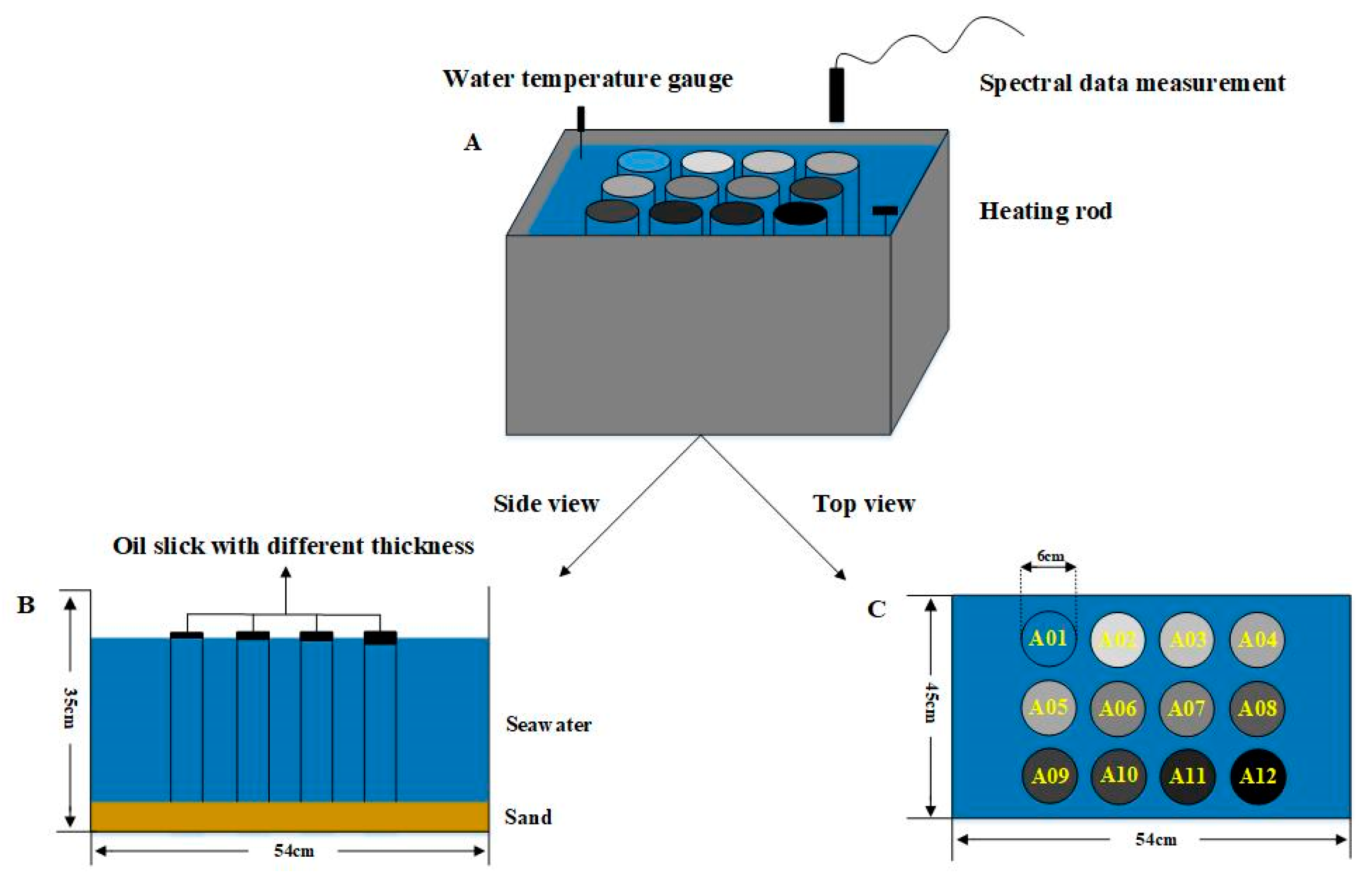
2. Data Collection and Processing

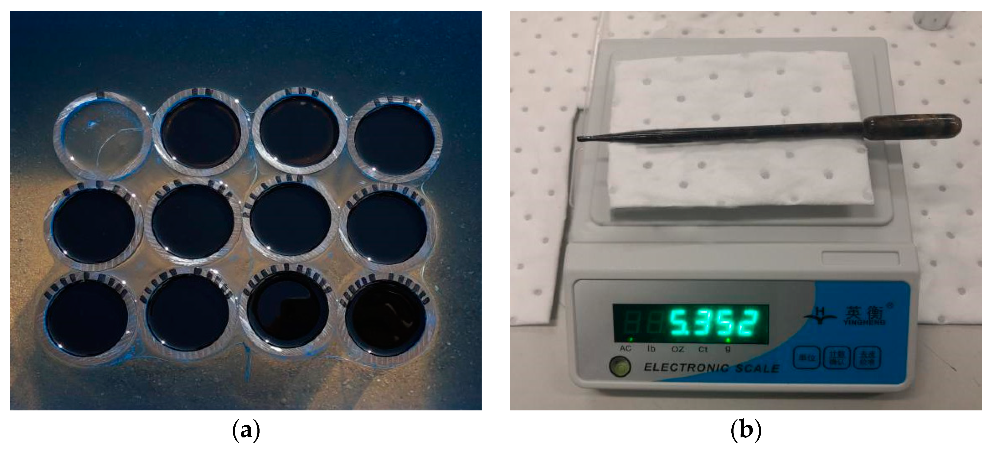
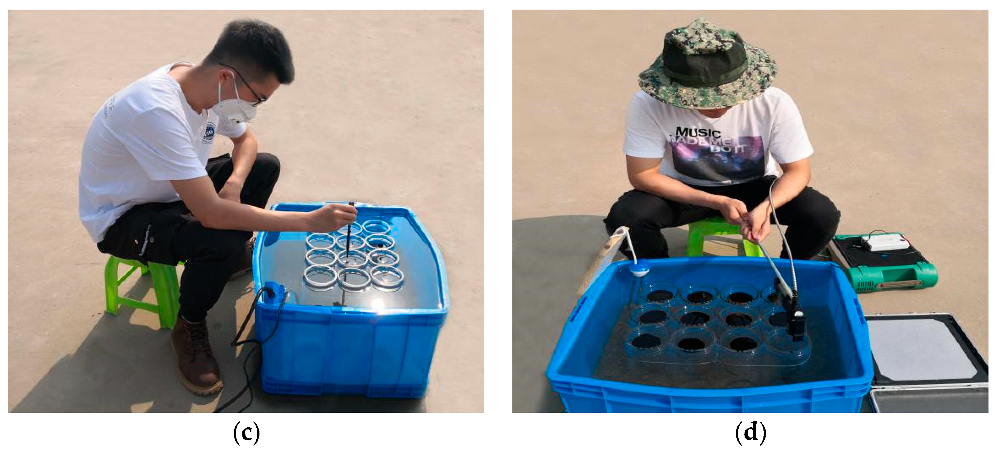
2.1. Data Acquisition

The experiment was conducted on November 8, 2019 in the First Institute of Oceanography of the Ministry of Natural Resources, China. Due to the short experimental observation time, the emulsification of crude oil was not considered. The oil used in the experiment was sour crude oil produced by the Shengli Oilfield located in Dongying, China. During the weathering process, oil undergoes physical and chemical changes such as spreading, drifting, mixing, evaporation, sedimentation, dissolution, emulsification, photo-oxidation, and biodegradation, thus forming different pollution types [29]. Due to the short time of this experiment designed, the weathering of oil was not considered in the experiment. The Analytical Spectral Devices (ASD)-FieldSpec4 spectroradiometer, which has been calibrated in the Anhui Institute of Optics, and precision machinery were used to carry out outdoor oil film thickness spectrum measurements. The spectral curve obtained in the experiment ranged from 350 nm to 2500 nm. The spectral resolution in the 350–1000 nm range is 3 nm, the spectral resolution in the 1001–2500 nm range is 7 nm, and the field angle of the spectroradiometer was set to 25°. We measured the oil film 10 cm above the surface of the seawater. The parameter settings of the ASD-FieldSpec4 spectroradiometer are shown in

Table 1. Parameters of the ASD-FieldSpec4 spectroradiometer.

Parameters	Index
Spectral range (nm)	350–2500
Spectral resolution (nm)	3@350–1000, 7@1001–2500
Spectral sampling interval (nm)	1.4@350–1000, 1.1@1001–2500
Field angle (°)	25
Wavelength accuracy (nm)	0.5
Scanning method	Fixed and moving grating combination spectroscopy
Stray light (nm)	0.02%@350–1000, 0.01%@1001–2500
Wavelength repeatability (nm)	0.1

Notes: Parameter of the ASD-FieldSpec4 spectroradiometer is from ASD user manual.

.

We simulated a near-real marine environment by adding sand to the bottom of a storage box and filling it with seawater. Through pre-experiments, we found that crude oil does not easily stick to the acrylic tube wall, which is also the reason why we chose acrylic tubes as the experimental container. Twelve acrylic tubes with an inner diameter of 6 cm were fixed in the storage box and functioned as containment devices to prevent the irregular diffusion of the oil films. We drilled holes into the walls of the containers to connect them, ensuring that the oil film was at the same water level. We labeled the containers 1 to 12, and experimental container 1 contained pure seawater as a control. Because this experiment was conducted in winter, the crude oil did not easily diffuse. Therefore, we used a heating rod to heat the seawater and slightly stirred the oil film to accelerate the diffusion rate and uniform distribution. The seawater was heated to about 35 °C, which is close to summer seawater temperatures. We measured the oil film after it was completely diffused and the experimental water was cooled to room temperature. The experimental observation setup is shown in Figure 1.

Before the measurement, we first carried out an accurate density measurement of the crude oil. We used an electronic scale to weigh the empty beaker mass. The manufacturer of the electronic scale is YingHeng from China, and the accuracy of the electronic scale is 0.001 g. We used 200 g standard weights which has been calibrated to calibrate the electronic scales before the experiment. Then, we used a dropper whose manufacturer is ShiDai in China to add crude oil of a known volume to a beaker (100 mL) and measured the beaker mass. Furthermore, we obtained the volume of the crude oil by reading the scale on the beaker wall. Based on the following formula for liquid density, we obtained the accurate density of the crude oil used in the experiment:

$${\rho }_{Oil}=\left(m_1-m_0\right)/V,$$

(1)

where ρ_Oil represents the accurate density of crude oil used in the experiment, m₀ is the mass of the empty beaker, m₁ represents the mass of the beaker after adding the crude oil, and V represents the volume of the beaker.

An electronic scale was used to weigh the empty dropper before adding the crude oil. We filled a dropper with crude oil and then measured the weight of the dropper. Next, we added the crude oil to experimental container 2. The dropper was 10–15 cm away from the water surface during dropping, and the dropping point remained near the center of the water surface of the experimental container. Then, we weighed the dropper again to obtain the accurate mass of crude oil dripped into the experimental container. After the oil film had completely diffused, we calculated the volume of crude oil dripped into the experimental container based on the density obtained from the previous crude oil density measurement experiment. According to the inner diameter of the acrylic tube used in the experiment, we obtained the absolute thickness of the oil film in experimental container 2, as follows.

$$h_{Oil}=\frac{M_a-M_b}{\mathsf{\pi }\cdot {\rho }_{Oil}\cdot r_{}^2}.$$

(2)

where M_a represents the mass of the dropper after being filled with crude oil, M_b is the mass of the dropper after adding the crude oil to the experimental container, ρ_Oil represents the accurate density of the crude oil, h_Oil is the absolute thickness of the oil film in the experimental container, and r represents the radius of the container. We repeated the above operation to calculate the thickness of the crude oil film in experimental containers 3 to 12. In this experiment, we set up a total of 12 experimental groups of oil films of different thicknesses from 0 to 2000 μm. Since the time of our experiment was in winter and the outdoor temperature was low, the oil film was not easy to diffuse. Furthermore, we found through the pre-experiment that the minimum complete diffusion thickness of the oil film was about 350 μm; thus, our thinnest oil film thickness was set as 372 μm at that time. The oil film thicknesses in the experimental groups are shown in

Table 2. Oil film thicknesses in the experimental groups.

No.	Oil Film Area (cm2)	Oil Film Quantity (g)	Oil Film Thickness (μm)
1	0.000	0.000	0.000
2	19.635	0.615	372
3	19.635	0.856	518
4	19.635	1.129	683
5	19.635	1.426	862
6	19.635	1.608	972
7	19.635	1.950	1179
8	19.635	2.282	1380
9	19.635	2.460	1487
10	19.635	2.752	1664
11	19.635	3.106	1878
12	19.635	3.239	1958

Notes: The calculated density of crude oil used in experiment is 0.842 g/mL.

.

The experimental spectra were measured between 11:00 and 13:00. We wanted to emulate a real oil spill scenario as much as possible, thus, we chose the sun as the light source. The wind speed was low and solar light was strong on the day of the experiment, which meets the criteria for spectrum measurements. We fully considered the characteristics of low remote sensing reflectance of the water body, and used the gray board (TD-MFB30-03Y-20), which has been calibrated by ASD-FRT and SolidSpec-3700 similar to Lambert body as the standard plate for measurement experiment. We preheated the ASD spectroradiometer for 15 min before measurement to ensure the accuracy of observation results and strictly followed the experimental observation standards. The integration times of ASD spectroradiometer was set to 0.05 s and the IFOV was set to 25°. During the measurement, the observers faced the sun and observed the oil film vertically to avoid casting a shadow onto the oil film. We observed the gray board at the beginning and the end of each observation experiment round to ensure the accuracy of the spectral curves of the gray board. We conducted two rounds of spectral data measurement on the oil film in each experimental group, and 20 spectral curves were measured in each round. Thus, we obtained a total of 480 spectral curves of oil films with different thicknesses (including 40 pure seawater spectral curves). Images of the field experiment are shown in Figure 2.

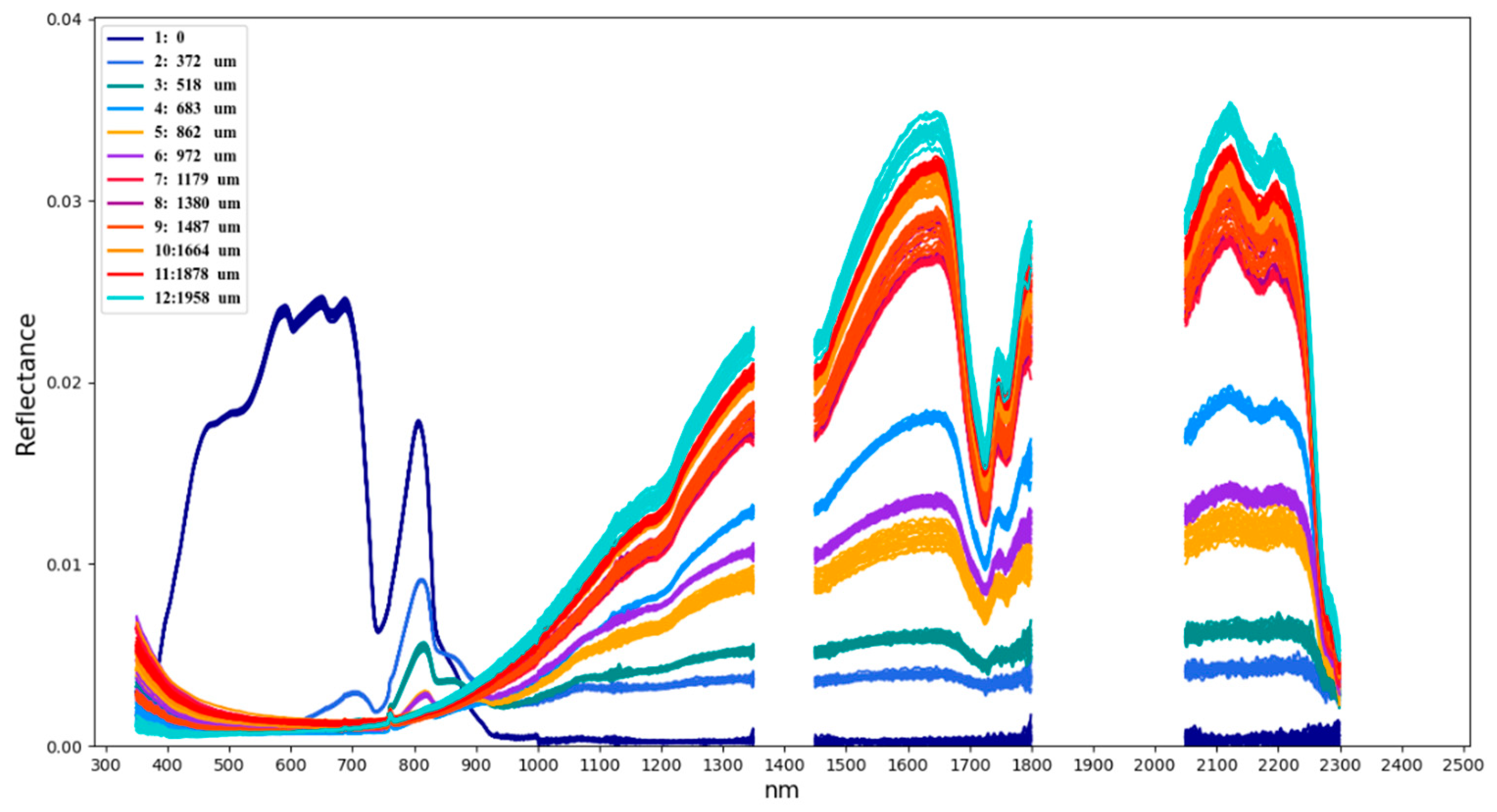
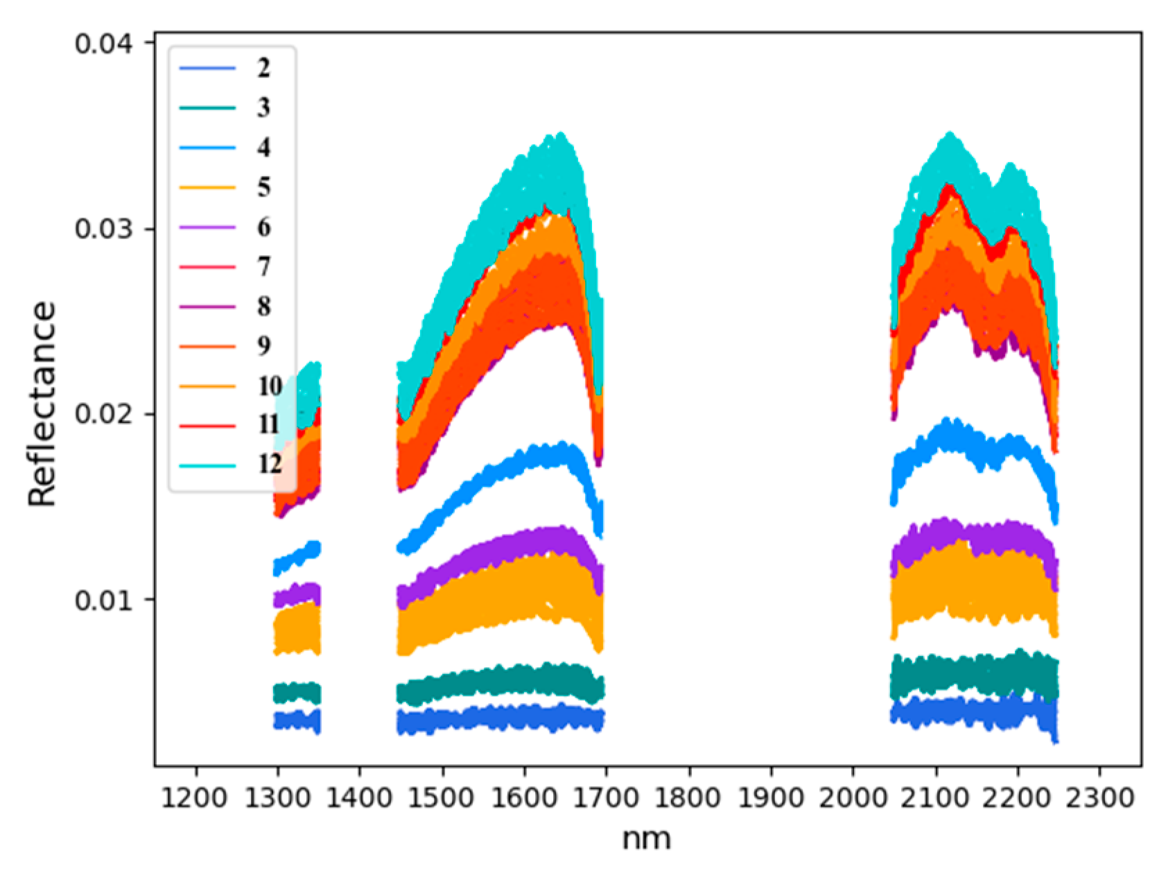
2.2. Spectral Data Processing

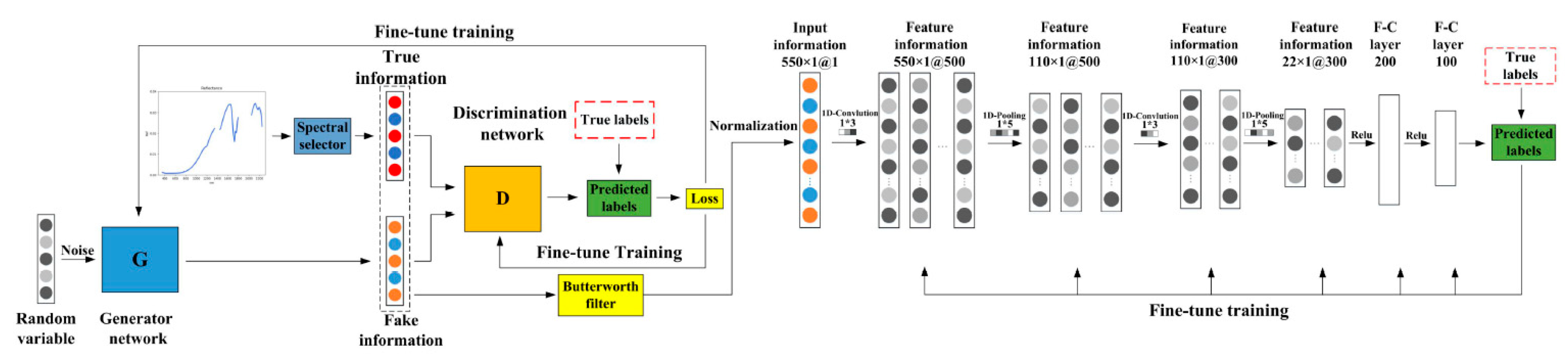
The spectral data obtained in this outdoor experiment consist of the radiance of the crude oil film and sky light, thus, it is necessary to convert the radiance into remote sensing reflectance to eliminate the effects of sky light. The formula for calculating the radiance of the oil film, ignoring external influences such as solar variability and sunglint, is as follows [30]:

$$L_w(\lambda ,\theta ,\varphi ;{\theta }_0,{\varphi }_0)=L_{sfc}(\lambda ,\theta ,\varphi ;{\theta }_0,{\varphi }_0)-\rho \cdot L_{sky}(\lambda ,\theta ,\varphi ;{\theta }_0,{\varphi }_0),$$

(3)

where λ is the wavelength, θ represents the zenith angle of the spectroradiometer, φ is the azimuth of the spectroradiometer, θ₀ represents the zenith angle of the sun, φ₀ is the azimuth of the sun, L_w(λ,θ,φ;θ_0,φ₀) represents the radiance of the crude oil film, L_sfc(λ,θ,φ;θ₀,φ₀) is the radiance measured by the spectroradiometer, ρ represents the oil-gas interface reflectance, and L_sky(λ,θ,φ;θ₀,φ₀) is the sky radiance.

The remote sensing reflectance is the ratio of the surface reflected energy to the incident energy reaching the surface. The formula for calculating the remote sensing reflectance is shown below:

$$R_{rs}(\lambda ,\theta ,\varphi )=\frac{L_w(\lambda ,\theta ,\varphi ;{\theta }_0,{\varphi }_0)\cdot {\rho }_p\left(\lambda \right)}{\mathsf{\pi }\cdot L_p\left(\lambda \right)}.$$

(4)

where R_rs(λ,θ,φ) represents the remote sensing reflectance, ρ_p(λ) is the standard plate reflectance, and L_p(λ) represents the standard plate radiance.

The measurement of oil films by the ASD spectroradiometer is greatly affected by the external environment. Hence, it is necessary to eliminate abnormal spectral curves that have been seriously disturbed by environmental factors such as wind and the change of observation distance. We performed batch remote sensing reflectance calculations on the measured spectral data. The remote sensing reflectances of seawater and oil films of different thicknesses in each experimental group are shown in Figure 3.

Because the spectral data in the channels 1350–1450 nm, 1800–2050 nm, and 2300–2500 nm are affected by the strong absorption of water vapor and spectrometer splice point offsets, abnormal fluctuations occurred; thus, we deleted the data. As shown in the figure, the remote sensing reflectance of the seawater is affected by the background of the fine sandy substrate and experiment device such as acrylic tubes and box. Hence, the spectral curve of the seawater shows abnormal jitter in the VNIR channels. Due to the thickness of the oil film in groups 2–4 is thin, the spectrum curve is significantly affected by the background of the sediment and experiment materials in the visible light channels. The oil film in groups 5–12 is thicker and has a stronger ability to absorb visible light, thus, the spectral curve is not easily affected by substrates. In addition, the spectral data of oil films of different thicknesses are poorly separable in the visible light channels and have good spectral separability in the NIR and SWIR channels. In these ranges, except for the fourth experimental group, which did not achieve a uniform thickness, the overall remote sensing reflectance of the oil film in the other experimental groups increased with increases in oil film thickness.

3. Model and Method

In recent years, deep learning has become a hot research field in remote sensing. Compared with traditional methods, it has stronger ability of feature extraction and sample expansion [31]. We combined the deep learning model with the practical application problem to solve the problem of insufficient spectral data and improve the inversion accuracy. The OG-CNN model proposed in this paper consists of a self-expanding module for crude oil film spectral feature data and an oil film absolute thickness inversion module as shown in Figure 4. The spectral feature data self-expanding module consists of a spectral feature filter, a GAN, and a Butterworth low-pass filter. We used the module to extract spectral feature intervals with high separability and then generate high-quality simulated spectral feature data based on the GAN to expand the number of samples. The 1D-CNN based absolute thickness inversion module extracts the feature information of spectral feature data corresponding to oil films of different thicknesses by means of one-dimensional convolution. Furthermore, a mapping between the thickness and spectral feature information was constructed to realize the inversion of the absolute thickness of the crude oil film.

3.1. Crude Oil Film Spectral Feature Data Self-Expanding Module

The spectral data obtained in the experiment included a large amount of spectral information with a large degree of redundancy. In addition, the separability of spectral data of different thicknesses in some channels was poor, which was not conducive to the accurate quantitative inversion of crude oil film thickness. Therefore, we added a spectral feature filter to the OG-CNN model and determined the best spectral feature intervals. We first averaged the spectral data of different experimental groups and then determined the separability of the intervals of oil films of different thicknesses based on the spectral feature filters. The spectral feature filter was constructed based on the spectral standard deviation threshold of the oil film spectral feature extraction method [32,33], as shown below:

$$\left|\overline{{\sigma }_{\lambda ,i,j}}\right|>\left\{\mathrm{SD}\right({\sigma }_{\lambda ,i})+\mathrm{SD}({\sigma }_{\lambda ,j}\left)\right\}.$$

(5)

where λ represents the band number, SD(σ_λ,i) is the standard deviation of the oil film remote sensing reflectance of group i, and SD(σ_λ,j) is the standard deviation of the oil film remote sensing reflectance of group j. Furthermore, $\left|\overline{{\sigma }_{\lambda ,i,j}}\right|$ represents the difference in oil film remote sensing reflectances of groups i and j at band λ. If $\left|\overline{{\sigma }_{\lambda ,i,j}}\right|$ is greater than the threshold, the interval is a spectral feature interval with better spectral separability.

A GAN includes a generative network (G) and a discriminative network (D). The purpose of G is to learn the distribution of real samples and generate synthetic samples with similarity to the real samples. The purpose of D is to determine the authenticity of the samples. Through adversarial training, D maximizes the discrimination of training sample sources and maximizes the similarity between real data and the data generated by G. The adversarial training process is as follows:

$$\underset{\mathrm{G}}{\min }\underset{\mathrm{D}}{\max }\mathrm{V}(\mathrm{D},\mathrm{G})={{\displaystyle \mathrm{E}}}_{\mathrm{X}~\mathrm{Pdata}\left(\mathrm{x}\right)}\left[\mathrm{lgD}\right(\mathrm{x}\left)\right]+{{\displaystyle \mathrm{E}}}_{\mathrm{X}~\mathrm{P}\left(\mathrm{z}\right)}\left[\lg \right(1-\mathrm{D}\left(\mathrm{G}\right(\mathrm{z}\left)\right)\left)\right].$$

(6)

During training to optimize D, when the input of D is a real sample x, the aim of the data self-expanding module is to modify D(x) so that it approaches 1. When the input sample of D is the generated sample G(z), the aim of the module is to modify D(G(z)) to approach 0, that is, 1-D(G(z)) tends to 1, thus, D is maximized. During training to optimize G, when the input information is random noise z, the aim of the module is to modify D(G((z)) to approach 1, that is, 1-D(G(z)) tends to 0, thus, the model G is minimized. If and only if P_z = P_data is there a globally optimal solution to the problem of maximizing the two-sided game, and the module reaches the Nash equilibrium point.

Because the spectral feature data generated by the data self-expanding module have a high level of jitter, we added a Butterworth low-pass filter to this module to perform smooth denoising on the generated samples and simulate the true spectral feature data to the greatest extent. A Butterworth filter is also called a maximally flat filter, and its amplitude and frequency are the flattest possible in the pass band (without fluctuations). In the stop band, the frequency amplitude gradually decreases to zero as the frequency increases. The Butterworth filter works as follows:

$$|H(w){|}^2=\frac{1}{1+{\epsilon }^2{\left(\frac{w}{w_p}\right)}^{2n}}=\frac{1}{1+{\left(\frac{w}{w_c}\right)}^{2n}}.$$

(7)

where n represents the order of the filter, w is the signal frequency, w_p represents the band edge frequency, and w_c is the normalized cut-off frequency

3.2. Crude Oil Film Absolute Thickness Inversion Module

This module is based on the real spectral feature data and the simulation data generated by the data self-expanding module to construct a mapping relationship between the spectral feature data and the absolute thickness of the oil film. We employed iterative training and hyperparameter tuning to realize the function of the module to invert the absolute thickness of the crude oil film. The structure of the crude oil film absolute thickness inversion module is shown in

Table 3. Structure of crude oil film absolute thickness inversion module.

Layer	Number	Kernel	Stride
Convolutional layer-1	500	1 × 3	1
Pooling layer-1	500	1 × 10	5
Convolutional layer-2	300	1 × 3	1
Pooling layer-2	300	1 × 10	5
Fully connected layer-1	200	—	—
Fully connected layer-2	100	—	—

. This module consists of two one-dimensional convolutional layers, two one-dimensional pooling layers, and two fully connected layers.

Instead of traditional convolution, 1D-CNN is based on a one-dimensional planar convolution kernel to convolve a one-dimensional information receptive field. The one-dimensional convolution layer is the core part of a 1D-CNN, has a strong multi-level feature expression ability, and can fit nonlinear data. The 1D-CNN extracts the feature information of the spectral feature data through the convolution process, reducing its redundancy. This approach also greatly reduces the number of model parameters and the complexity of calculation by means of its sparse expression and weight sharing. The calculation process is as follows:

$${{\displaystyle h}}_{i,j}=g\left({\displaystyle \sum _m^M({{\displaystyle h}}_{i-1,m}\times {{\displaystyle w}}_{i,mj})+{{\displaystyle b}}_{i,j}}\right).$$

(8)

where h_i,j represents the j^th output feature map of the i^th convolution layer, M is the number of feature maps of the i^th convolution layer, w_i,mj represents weight, b_i,j is bias, and g(f) represents the activation function.

We chose the rectified linear unit (ReLU) function as the activation function of the oil film absolute thickness inversion module. This function enables the thickness inversion module to perform gradient descent more efficiently while maintaining a fast calculation speed, and can avoid the phenomena of gradient disappearance and gradient expansion. The formula for calculating the ReLU function is as follows:

$$g\left(x\right)=\max (0,x).$$

(9)

The pooling method of the module is one-dimensional maximum pooling. This module reduces the risk of overfitting and enhances the robustness of the module through the pooling process. Each pooling layer corresponds to the receptive field of the convolutional layer of size n × 1. The maximum pooling formula is as follows:

$$a_j=\underset{N\times 1}{\max }(a_i^{n\times 1}\mathrm{u}(n,1\left)\right).$$

(10)

where max() represents the one-dimensional maximum pooling function, u(n,1) is the window function of the convolution layer, and a_j is the maximum value in the neighborhood.

The reverse fine-tuning process of the module uses the backpropagation (BP) algorithm. The module combines the measured oil film thickness data to adjust the overall weight and paranoia of the module layer by layer so that the module’s mapping for different oil film thicknesses is optimized.

4. Results and Discussion

4.1. Accuracy Evaluation Indices

In this paper, the mean relative error (MRE) was selected as the loss function of the OG-CNN model. To show the inversion results of the model and change trends more intuitively, we chose mean relative accuracy (MRA) as the evaluation index of the thickness inversion accuracy of the OG-CNN model and we chose the determination coefficient (R²) to evaluate the goodness of fit of the model:

$$\mathrm{MRE}=\frac{1}{N}{\displaystyle \sum _{i=1}^N|\frac{h\left(x_i\right)-\widehat{h}}{\widehat{h}}|}\times 100\%.$$

(11)

$$\mathrm{MRA}=(1-\frac{1}{N}{\displaystyle \sum _{i=1}^N|\frac{h\left(x_i\right)-\widehat{h}}{\widehat{h}}|})\times 100\%.$$

(12)

$${\mathrm{R}}^2=1-\frac{{\displaystyle \sum _{i=1}^N{\left(h\right(x_i)-\widehat{h})}^2}}{{\displaystyle \sum _{i=1}^N{\left(h\right(x_i)-\overline{h})}^2}}.$$

(13)

where N represents the number of test samples, h(x_i) is the predicted inversion value, ĥ represents the true value, and h is the average value.

We chose mean deviation (MD) to evaluate the stability of the oil film thickness inversion results of the OG-CNN model. A larger MD value indicates more jitter in the model and worse model stability. Its calculation formula is as follows:

$$\mathrm{MD}=\frac{1}{M}{\displaystyle \sum _{i=1}^M\left|g\right(x_i)-\overline{g}|}.$$

(14)

where M represents the number of inversion experiments, g(x_i) is a single inversion result of the model, and g represents the average of the multiple inversion results of the model.

4.2. Spectral Feature Filter Experiment

In this experiment, the ASD-FieldSpec4 spectroradiometer was used to carry out outdoor oil film thickness spectrum measurements. The spectral data obtained in the experiment totaled 2151 channels. Moreover, there was a large amount of redundant information and a heavy GPU throughput burden. In addition, the spectral curves of the oil films of different thicknesses in some spectral intervals are poorly separable, which is not conductive to the accurate inversion of oil film thickness. Therefore, we equipped the OG-CNN model with a spectral filter to determine spectral feature intervals that respond distinctively to oil films of different thicknesses. We performed spectral feature interval analysis on the spectral curves of the 11 oil film experimental groups in pairs. Furthermore, we performed an intersection operation on the selected spectral feature intervals, and the results are shown in

Table 4. Spectral feature filtering experimental results.

No.	Spectral Feature Intervals (nm)
1	350–359
2	1300–1349
3	1450–1694
4	1775–1799
5	2050–2246

.

As shown in Figure 5, the correspondence between the spectral data in the 350–359 nm range and the oil film thickness data is confusing, and the separability is not very strong. In addition, 350–359 nm belongs to the ultraviolet range, and the spectral data in the ultraviolet range are more sensitive to thin oil films and less sensitive to thick oil films. The separability of thin oil films is obvious in 1775–1799 nm, while the separability of thick oil film is relatively poor; thus, we artificially eliminate the data in this interval. According to the results of the spectral feature filtering, we selected the spectral data in the 1300–1349 nm, 1450–1694 nm, and 2050–2246 nm channels as the spectral feature data of the oil film thickness inversion experiment after excluding the intervals with less spectral information. The spectral feature intervals are shaded in gray in Figure 5.

In this experiment, we obtained a total of 440 spectral total measurements at 11 different thicknesses. We divided the filtered spectral feature data into training samples and test samples with a ratio of 2:1 to train the OG-CNN model and evaluate model inversion accuracy. We carried out five repeated inversion experiments to ensure the accuracy of model inversion. By comparing the inversion results of full-band spectral data, we explored whether using the spectral feature filter is necessary. The experimental results are shown in

Table 5. Spectral feature filter experiment inversion results.

Experimental Data	Inversion Results of Oil Film Thickness (%)			Time (s)
	MRA (Single Experiment)	MRA + MD	R2
Full band spectral data	90.45/90.32/90.31/90.44/90.38	90.38 ± 0.05	0.928	290.1
Spectral characteristic data	94.80/94.74/94.76/94.73/94.82	94.77 ± 0.03	0.961	80.2

.

As shown in Table 5, the accuracy of the model based on the filtered spectral feature data is 94.77%, the R² is 0.961 and its MD is ±0.03%. Compared with the results of the model based on full-band spectral data, the inversion accuracy is improved by 4.39%, the R² is improved by 0.033 and the model shows good stability. In addition, the model based on filtered spectral feature data takes only 80.2 s to compute on a NVIDIA GTX1050, which is much lower than the 290.1 s required for the model using full-band data, greatly reducing the experimental time and hardware burden. Therefore, we can conclude that the OG-CNN model with the spectral feature filter can effectively eliminate redundant information in spectral data, improve the inversion accuracy of the model, reduce the amount of calculation required, and accelerate the model’s convergence speed.

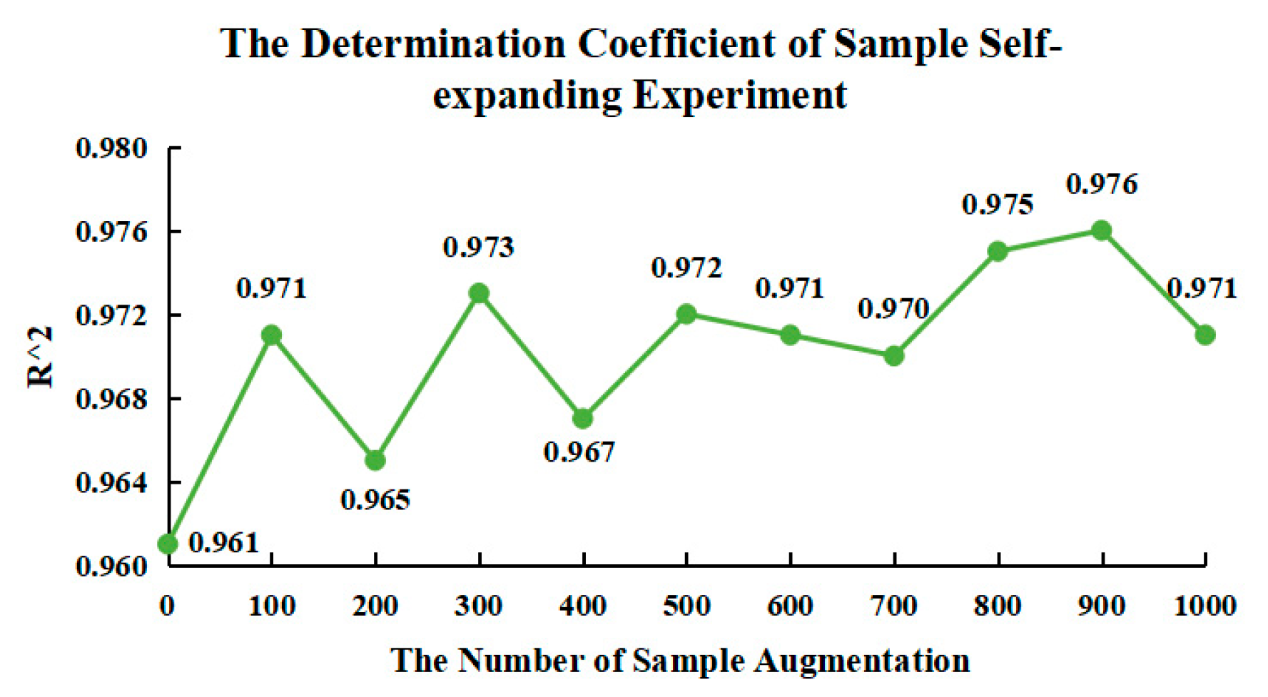
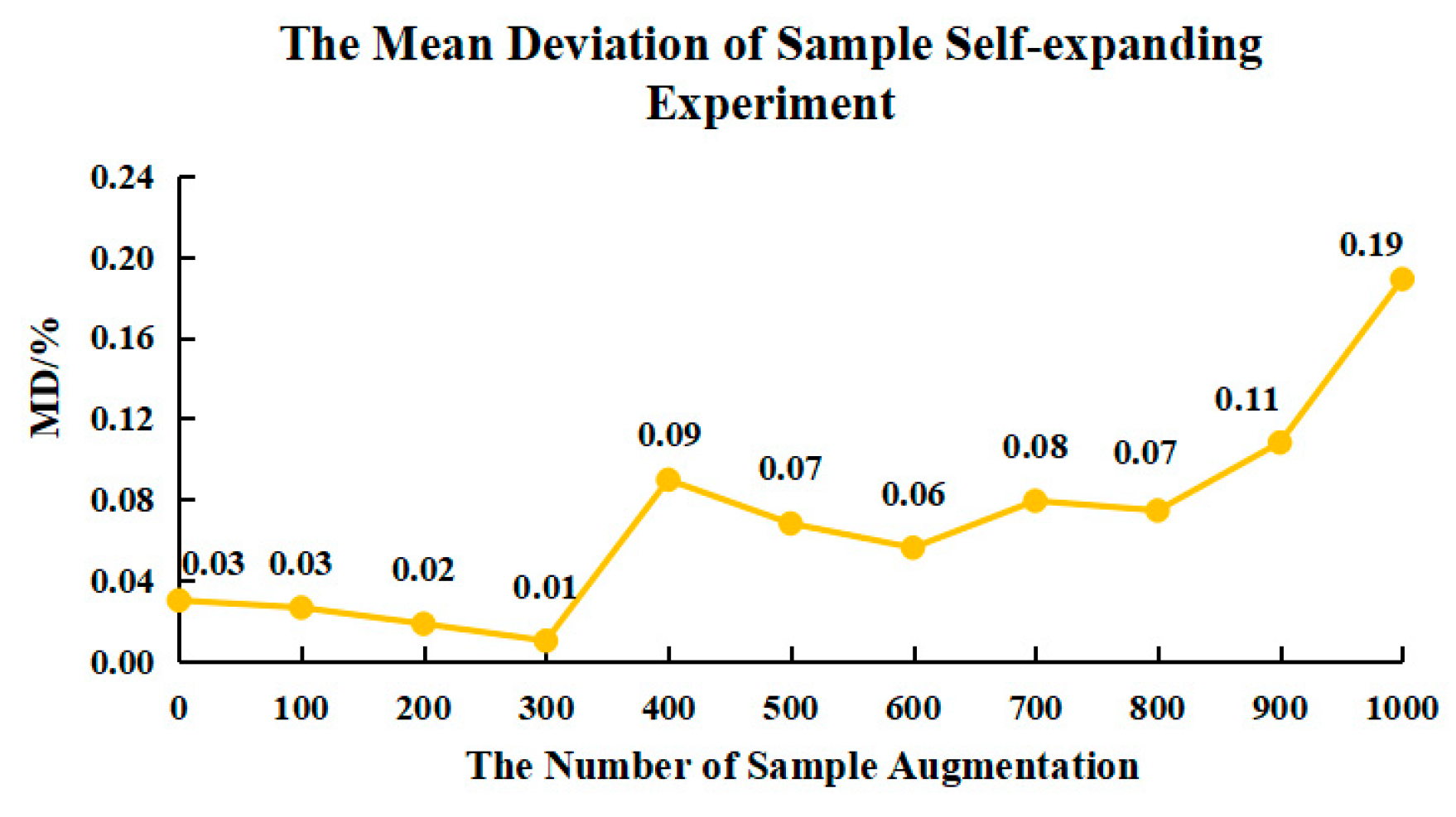
4.3. Sample Data Self-Expanding Experiment

In the current stage of this research, most of the absolute thickness data of crude oil films were obtained under outdoor favorable conditions, and the amount of data obtained was limited. Moreover, the inversion of the absolute thickness of the oil film requires the support of a large amount of data. The OG-CNN model proposed in this paper can generate high-quality simulated crude oil film spectral feature data based on the GAN’s adversarial training process. Through the data self-expanding process of the model, it can enrich the diversity of the samples and enhance the generalization ability, thereby improving the inversion accuracy of the model. After fully considering the accuracy in the pre-experiment, the stability and the goodness of fit of the model, we varied the number of self-expanding samples to range from 0 to 1000 (for a total of 11 experimental groups) to explore the number of augmented samples with the best inversion results. The sample data self-expanding experiment inversion results are shown in

Table 6. Sample data self-expanding experiment inversion results.

Number	Inversion Results of Oil Film Thickness (%)			Time (s)
	MRA (Single Experiment)	MRA + MD	R2
0	94.80/94.74/94.76/94.73/94.82	94.77 ± 0.03	0.961	80.2
100	96.10/96.05/96.12/96.13/96.14	96.11 ± 0.03	0.971	95.6
200	95.95/95.96/96.00/95.96/95.99	95.97 ± 0.02	0.965	109.2
300	96.36/96.35/96.34/96.36/96.36	96.35 ± 0.01	0.973	125.5
400	96.28/96.33/96.13/96.05/96.17	96.19 ± 0.09	0.967	141.3
500	96.38/96.56/96.45/96.36/96.35	96.42 ± 0.07	0.972	154.2
600	96.25/96.39/96.46/96.45/96.40	96.39 ± 0.06	0.971	172.7
700	96.49/96.44/96.35/96.35/96.60	96.45 ± 0.08	0.970	187.3
800	96.89/96.75/96.75/96.90/96.72	96.80 ± 0.07	0.975	199.8
900	96.76/96.73/96.80/96.41/96.70	96.68 ± 0.11	0.976	212.4
1000	96.50/96.63/96.14/93.87/96.43	96.51 ± 0.19	0.971	227.9

.

As shown in Table 6, as the number of self-expanding samples increases, the computational burden increases and the time of inversion experiment also increases. As shown in Figure 6, within a certain range, the inversion accuracy of the model as a whole increases with the number of self-expanding samples. As shown in Figure 6 and Figure 7, when the number of samples is 800, the R² of the model reaches 0.975, and the inversion accuracy reaches a peak of 96.80%, which then shows a downward trend. Compared with the experimental results before the sample self-expanding operation, the inversion accuracy of the model has improved by 2.03%. As shown in Figure 8, the overall stability of the OG-CNN model decreases with increasing sample size. When the sample size is 1000, the MD of the inversion results reaches ±0.19%, and the model shows strong levels of jitter.

Therefore, we can conclude that within a certain range, as the number of self-expanding samples increases, the diversity of samples is enhanced. To some extent, it can enrich the generalization of the model, improve the accuracy of inversion and optimize the fitting degree of the model. However, this does not mean that a larger number of samples is better. After the number of augmented samples exceeds 800, the OG-CNN model begins to overfits the data, and the inversion accuracy decreases accordingly. In addition, although the OG-CNN model can perform sample self-expansion based on measured data, the spectral feature data generated by the process is not really equivalent to real spectral feature data. Although the inversion accuracy of the model can be improved within a certain range, the stability of the model will inevitably decrease as the amount of simulated data generated increases.

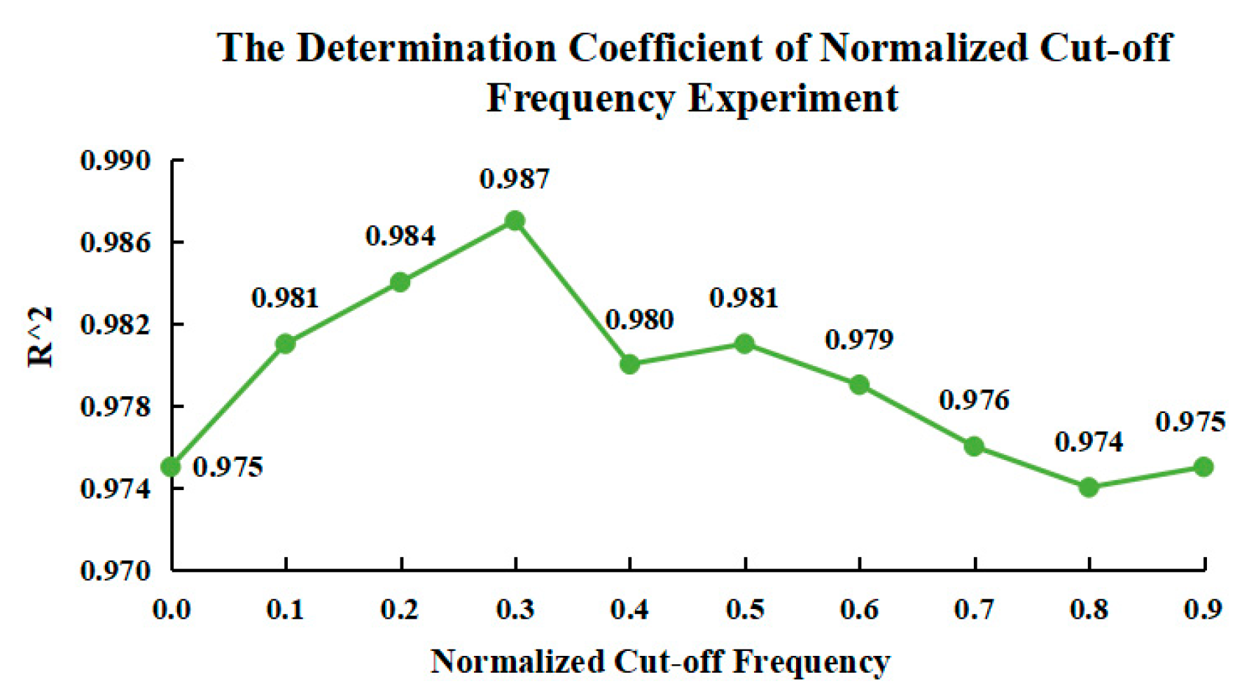
4.4. Spectral Feature Filter Experiment

As a kind of generative neural network, GAN has a certain degree of volatility when simulating real sample data through the adversarial training process. Therefore, we added a Butterworth low-pass filter after the GAN to filter the generated data to ensure that the generated simulated data are as close to the real spectral feature data as possible to improve the accuracy of the oil film thickness inversion. As shown in Figure 9 and Figure 10, after the sample self-expansion and filtering (the normalized cut-off frequency was set to 0.1), the generated spectral feature data represents well the spectral trends of the true spectral feature data and the spectral differences between different thicknesses of oil films.

To ensure the performance of the filters, we uniformly set the order of the filters to 10. We explored the necessity of using Butterworth filters by adjusting the normalized cut-off frequency and comparing the results of the oil film thickness inversion model. The experimental results are shown in

Table 7. Inversion results for various values of normalized cut-off frequency.

Parameter	Inversion Results of Oil Film Thickness (%)			Time (s)
	MRA (Single Experiment)	MRA + MD	R2
0	96.66/96.75/96.75/96.63/96.72	96.80 ± 0.07	0.975	199.8
0.1	97.43/97.51/97.64/97.44/97.14	97.43 ± 0.12	0.981	199.5
0.2	98.01/98.02/98.07/98.20/98.14	98.09 ± 0.07	0.984	199.2
0.3	98.17/98.01/98.16/98.07/98.18	98.12 ± 0.06	0.987	198.3
0.4	97.54/97.50/97.54/97.49/97.49	97.51 ± 0.02	0.980	198.7
0.5	98.08/97.77/97.82/97.90/98.08	97.93 ± 0.12	0.981	197.9
0.6	97.75/97.74/97.73/97.66/97.82	97.74 ± 0.04	0.979	196.7
0.7	97.71/97.79/97.19/97.05/97.33	97.41 ± 0.27	0.976	197.7
0.8	96.86/96.97/96.95/96.93/96.96	96.93 ± 0.03	0.974	197.5
0.9	97.03/97.08/97.00/96.97/96.98	97.01 ± 0.03	0.975	197.4

.

As shown in Table 7, when we set the normalized cut-off frequency of the Butterworth low-pass filter to 0.3, the inversion accuracy of the OG-CNN model reaches a peak of 98.12%, the R² remains at 0.980, and the MD of the inversion results is only ±0.06%, showing better model stability. When the normalized cut-off frequency is set to 0.7, the MD of the model inversion results reaches ±0.27%, and the model jitter is severe. It can be seen from Figure 11 and Figure 12 that after a Butterworth filter is added to the OG-CNN model, the inversion results of the oil film thickness and R² are substantially improved. In addition, when the normalized cut-off frequency is set to 0.3, the MD of the model’s inversion results is slightly improved compared with the model without the filter as shown in Figure 13, which effectively suppresses the jitter that may occur during the use of the model.

It can be concluded that using the Butterworth low-pass filter in the sample self-expanding module can greatly improve the accuracy of the model’s oil film thickness while ensuring the stability of the OG-CNN model. When the normalized cut-off frequency is set to 0.3, the filter can effectively filter the simulated spectral feature data generated by the sample self-expanding module to generate training samples that are the closest to the true spectral feature data, thereby improving the inversion accuracy and the goodness of fit of the OG-CNN model.

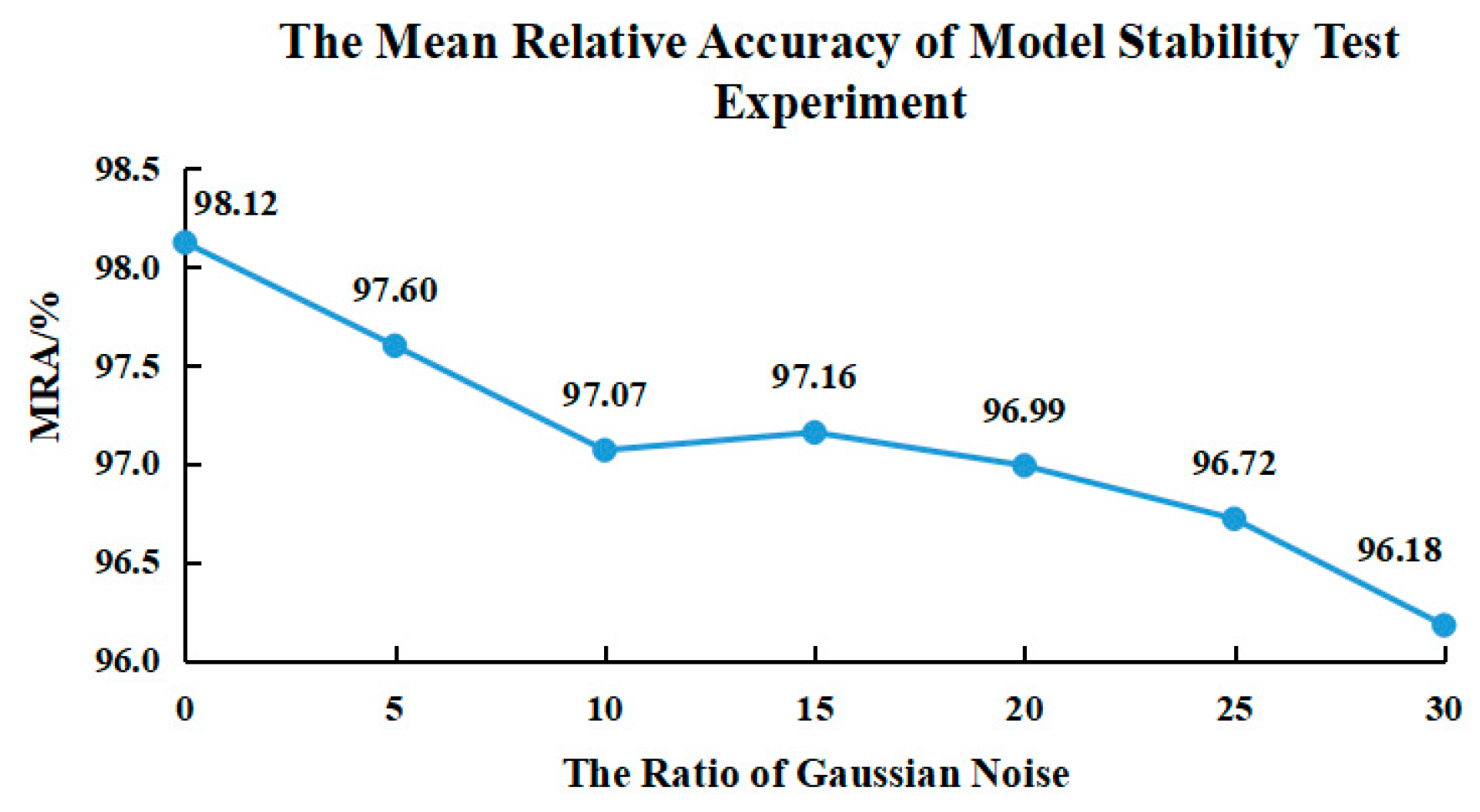
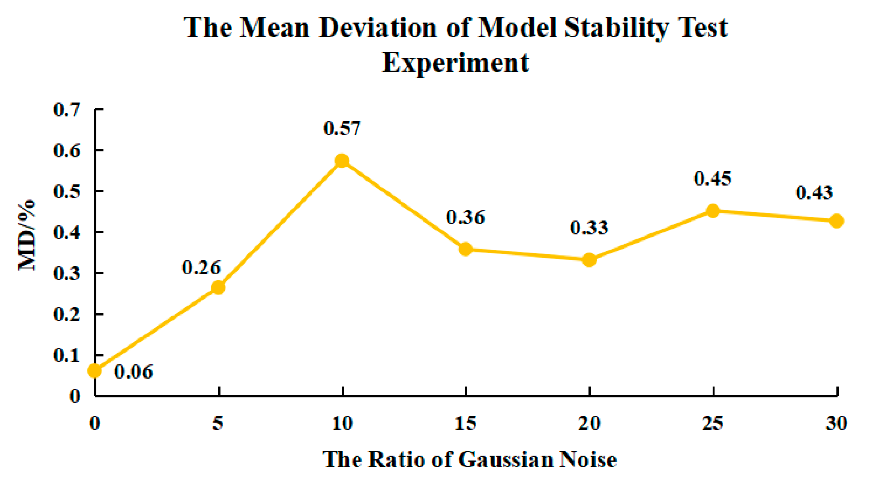
4.5. Model Stability Evaluation

Because the experimental environment is relatively ideal, to verify the inversion ability of the OG-CNN model under complex conditions, we randomly added 5%, 10%, 15%, 20%, 25%, and 30% Gaussian random noise to the spectral feature data. In this way, we simulated external environment interference to analyze the robustness of the model. The experimental results are shown in

Table 8. Model stability test experiment inversion results.

Gauss	Inversion Results of Oil Film Thickness (%)			Time (s)
	MRA (Single Experiment)	MRA + MD	R2
0	98.17/98.01/98.16/98.07/98.18	98.12 ± 0.06	0.987	198.3
5	97.43/97.87/97.51/97.98/97.19	97.60 ± 0.26	0.981	198.4
10	96.34/97.55/97.36/97.44/97.64	97.27 ± 0.57	0.979	198.4
15	96.29/97.13/97.76/97.24/97.36	97.16 ± 0.36	0.980	198.2
20	96.84/97.14/96.31/97.15/97.50	96.99 ± 0.33	0.976	198.8
25	96.47/95.84/96.83/96.86/97.59	96.72 ± 0.45	0.975	199.2
30	95.53/95.90/96.88/96.04/96.54	96.18 ± 0.43	0.973	199.1

.

As shown in Figure 14 and Figure 15, as the proportion of Gaussian noise increases, the inversion accuracy of the OG-CNN model shows a downward trend overall. When the proportion of Gaussian noise reaches 30%, the inversion accuracy of the model decreases to 96.18% and R² decreases to 0.973. In addition, as the proportion of noise increases, the overall jitter of the model increases, and the instability of the model also increases. As shown in Figure 16, when the proportion of Gaussian noise reaches 10%, the jitter of the model is the most severe, and the MD of the inversion results reaches ±0.57%, but the inversion accuracy of 97.07% is still maintained.

It can be concluded that although the OG-CNN model is affected by external noise, the experimental results of oil film thickness inversion will be affected to some extent, and the stability of the model will be weakened. However, the model can well suppress the influence of external interference factors, ensure the normal convergence of the model, stably maintain the inversion accuracy above 96% and an R² above 0.95, and control the MD within ±0.6. In this experiment, the inversion results and overall stability of the OG-CNN model are satisfactory, showing excellent robustness of the model.

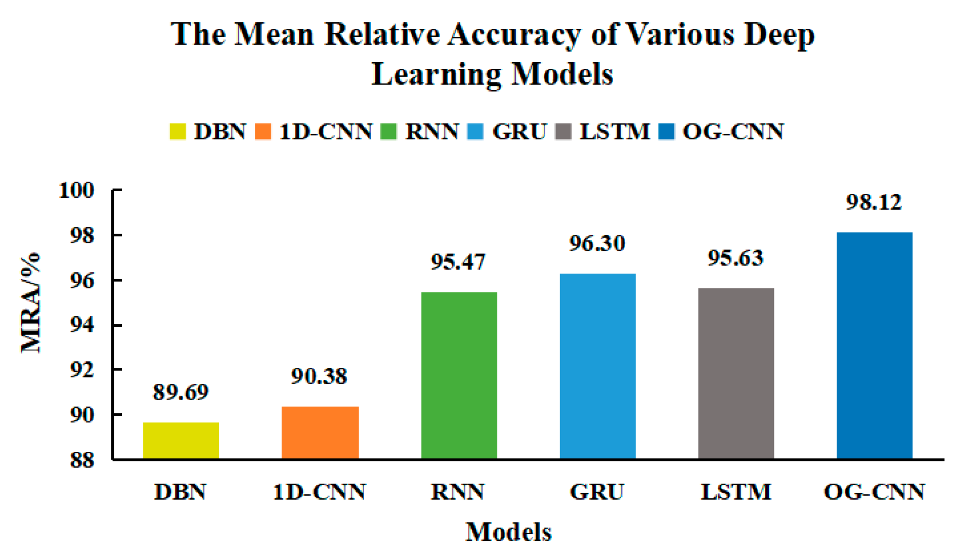
4.6. Comparison with Various Deep Learning Models

The oil film spectral feature information is one-dimensional information. Deep learning models such as DBN, 1D-CNN, RNN, GRU, and LSTM are widely used in one-dimensional signal processing. Under the same experimental conditions, the inversion results were compared with those models. The inversion results are shown in

Table 9. Inversion results for various deep learning models.

Model	Inversion Results of Oil Film Thickness (%)			Time (s)
	MRA (Single Experiment)	MRA + MD	R2
DBN	89.75/89.78/89.66/89.66/89.61	89.69 ± 0.06	0.918	150.6
1D-CNN	90.45/90.32/90.31/90.44/90.38	90.38 ± 0.05	0.928	290.1
RNN	95.46/95.47/95.81/95.41/95.22	95.47 ± 0.13	0.967	120.6
GRU	96.52/96.53/95.79/96.37/96.30	96.30 ± 0.21	0.968	123.1
LSTM	94.91/95.71/95.72/95.71/96.10	95.63 ± 0.29	0.965	124.3
OG-CNN (proposed)	98.17/98.01/98.16/98.07/98.18	98.12 ± 0.06	0.987	198.3

.

It can be seen from Table 9 that, compared with the traditional 1D-CNN model, the OG-CNN model proposed in this paper greatly shortens the inversion time and improves the efficiency of the oil film thickness inversion experiment. However, the OG-CNN model is limited to the one-dimensional convolution feature extraction method, and the convergence rate of the model is lower than that of RNN, GRU, and LSTM.

It can be seen from the Figure 17 and Figure 18 that the OG-CNN model’s inversion accuracy and goodness of fit for oil film thickness are higher than those of other types of deep learning models. Recurrent neural networks such as GRU also have good inversion results, while traditional 1D-CNN and DBN models perform poorly in the inversion experiment and have low inversion accuracy.

In addition, the OG-CNN model has excellent inversion capabilities while maintaining satisfactory stability as shown in Figure 19. The jitter of the model is only higher than that of the traditional 1D-CNN model. The OG-CNN model generates simulation data based on the self-expanding module, which enriches the diversity of samples while increases the instability of the model. The experimental results show that the OG-CNN model can well suppress the influence of sample expansion during the model convergence process, and output stable inversion experimental results.

5. Conclusions

It is of great importance to combine deep learning and remote sensing technology to accurately invert the thickness of the sea surface oil film to obtain information about sea surface oil spills. In this experiment, an outdoor experimental setup was built to simulate the near-real marine environment and obtain spectral data of crude oil film that is close to that of real scenarios. Furthermore, not all spectral data are conducive to the accurate inversion of the absolute thickness of the oil film. Some data with poor separability will interfere with the inversion process of the model and reduce the inversion accuracy. The OG-CNN model proposed in this paper can automatically filter the spectral feature intervals with better spectral response based on the spectral feature filter, which improves the model’s inversion accuracy and reduces the calculation cost. In addition, the model can perform sample self-expansion based on measured spectral data. By increasing the diversity of samples, the generalization and inversion accuracy of the model can be improved, and the problem of insufficient field measured data at the current stage can be effectively solved. In contrast to traditional modeling inversion methods, the model can fully extract the spectral characteristics of spectral feature data based on the 1D-CNN model, effectively avoid the useful spectral information loss in the previous method, and ensure the inversion accuracy of the model. The experimental results show that the OG-CNN model proposed in this paper has excellent performance in terms of thickness inversion results and model stability. Compared with other deep learning models, the OG-CNN model has obvious advantages in inversion accuracy. Therefore, it is technically feasible to apply this method to the inversion study of sea surface oil film thickness in marine oil spill disasters in the future. In future studies, we will migrate the inversion model to high spatial and spectral resolution remote sensing data of UAV to suppress the interference of mixed pixel and inverse the absolute thickness of the oil film with irregular diffusion on the real sea surface.

This experiment is only a basic research on the inversion of the absolute thickness of the oil film. Due to the short observation time of this experiment, we did not consider the emulsification of crude oil. In addition, the emulsification of crude oil takes time. This experiment was devoted to building an oil film thickness inversion model to obtain non-emulsified oil spills before oil emulsification. In the future, we will consider the emulsification and C-H absorption characteristics of crude oil in the inversion experiment of the oil film thickness. In the next phase of the research, we will use more accurate instruments for measuring the density of crude oil to achieve better film thickness accuracy calculations for comparison to the model thickness values. Moreover, this experiment was performed in winter, the temperature of the water was low, and the experimental environment lacked real sea wind and waves, thus, it was not easy for the crude oil film to spread. Therefore, we heated the water and stirred the oil film to speed up the diffusion process and shorten experiment time, then carried out the measurements when the water had cooled to room temperature. After heating the water, the oil absorbed heat and the temperature rose, which led to an increase in the remote sensing reflectances in the NIR and SWIR channels of the oil film. Even when water had cooled to room temperature, the oil film’s spectral curve was slightly different, which may be affected by water heating-induced loss of volatiles, thereby decreasing the slick volume. The temperature of oil spills on the sea surface will increase under long-term exposure to sunshine, and the oil spill temperature in the surrounding sea also will increase after explosions and fires in some oil fields, thus affecting the spectral curve of the oil film. Therefore, it is necessary to conduct a controlled experiment of natural oil film diffusion to explore the influence of water temperature on the crude oil film spectral curves and the results of oil film thickness inversion experiments.

References

1. Leifer, I.; William, J.L.; Simecek-Beatty, D.; Bradley, E.; Clark, R.; Dennison, P.; Hu, Y.; Matheson, S.; Jones, C.E.; Holt, B.; et al. State of the art satellite and airborne marine oil spill remote sensing: Application to the BP Deepwater Horizon oil spill. Remote Sens. Environ. 2020, 124, 185–209. [Google Scholar] [CrossRef] [Green Version]
2. Fingas, M.; Brown, C. Review of oil spill remote sensing. Mar. Pollut Bull. 2014, 83, 9–23. [Google Scholar] [CrossRef] [Green Version]
3. Yang, J.F.; Wan, J.H.; Ma, Y.; Zhang, J.; Hu, Y.B.; Jiang, Z.C. Oil spill hyperspectral remote sensing detection based on DCNN with multi-scale features. J. Coast. Res. 2019, 90, 332–339. [Google Scholar] [CrossRef]
4. del Frate, F.; Petrocchi, A.; Lichtenegger, J.; Calabresi, G. Neural networks for oil spill detection using ERS-SAR data. IEEE Trans. Geoence Remote Sens. 1999, 38, 2282–2287. [Google Scholar] [CrossRef] [Green Version]
5. Ferraro, G.; Baschek, B.; de Montpellier, G.; Njoten, O.; Perkovic, M.; Vespe, M. On the SAR derived alert in the detection of oil spills according to the analysis of the EGEMP. Mar. Pollut. Bull. 2010, 60, 91–102. [Google Scholar] [CrossRef]
6. Solberg, A.S.; Storvik, G.; Solberg, R.; Volden, E. Automatic detection of oil spills in ERS SAR images. Ieee Trans. Geoence Remote Sens. 1999, 37, 1916–1924. [Google Scholar] [CrossRef] [Green Version]
7. Keramitsoglou, I.; Cartalis, C.; Kiranoudis, C.T. Automatic identification of oil spills on satellite images. Environ. Model. Softw. 2016, 21, 640–652. [Google Scholar] [CrossRef]
8. Garcia-Pineda, O.; Macdonald, I.; Hu, C.; Svejkovsky, J.; Hess, M.; Dukhovskoy, D.; Morey, S.L. Detection of floating oil anomalies from the deep water horizon oil spill with synthetic aperture radar. Oceanography 2013, 26, 124–137. [Google Scholar] [CrossRef] [Green Version]
9. Topouzelis, K.; Psyllos, A. Oil spill feature selection and classification using decision tree forest on SAR image data. Isprs J. Photogramm. Remote Sens. 2012, 68, 135–143. [Google Scholar] [CrossRef]
10. Fingas, M. A literature review of the physics and predictive modelling of oil spill evaporation. J. Hazard. Mater. 1995, 42, 157–175. [Google Scholar]
11. FanG, S.A.; Huang, X.X.; Yin, D.Y.; Xu, C.; Feng, X.; Feng, Q. Research on the ultraviolet reflectivity characteristic of simulative targets of oil spill on the ocean. Spectrosc. Spectr. Anal. 2010, 30, 738–742. [Google Scholar]
12. Hu, J.C.; Wang, D.F. Monitoring method of ocean oil spilling based on remote sensing. Environ. Prot. Sci. 2014, 40, 68–73. [Google Scholar]
13. Ren, G.B.; Guo, J.; Ma, Y.; Luo, X.D. Oil spill detection and slick thickness measurement via UAV hyperspectral imaging. Haiyang Xuebao 2019, 41, 146–158. [Google Scholar]
14. Wu, X.D.; Song, J.M.; Li, X.G. Technical methods for marine oil spill quantity capture. Mar. Technol. 2011, 30, 50–54. [Google Scholar]
15. Song, S.S.; An, W.; Li, J.W.; Zhao, Y.P.; Jin, W.W. Review on the methods for assessment of marine oil spill volume. Coast. Eng. 2017, 36, 83–88. [Google Scholar]
16. Sun, S.; Hu, C.M. The challenges of interpreting oil-water spatial and spectral contrasts for the estimation of oil thickness: Examples from satellite and airborne measurements of the deepwater horizon oil spill. IEEE Trans. Geoence Remote Sens. 2019, 5, 1–16. [Google Scholar] [CrossRef]
17. Liu, B.X. Extraction and Analysis of Water Oil Film Based on Hyperspectral Characteristics. Ph.D. Thesis, Dalian Maritime University, Dalian, China, 2013. [Google Scholar]
18. Lu, Y.C.; Zhan, W.F.; Hu, C.M. Detecting and quantifying oil slick thickness by thermal remote sensing: A ground-based experiment. Remote Sens. Environ. 2016, 181, 207–217. [Google Scholar] [CrossRef]
19. Lu, Y.C.; Tian, Q.J.; Wang, X.Y.; Zheng, G.; Li, X. Determining oil slick thickness using hyperspectral remote sensing in the Bohai Sea of China. Int. J. Digit. Earth 2013, 6, 76–93. [Google Scholar] [CrossRef]
20. Jiang, Z.C.; Ma, Y.; Jiang, T.; Chen, C. Research on the extraction of red tide hyperspectral remote sensing based on the deep belief network. J. Ocean. Technol. 2019, 38, 1–7. [Google Scholar]
21. Chen, Y.S.; Jiang, H.L.; Li, C.Y.; Jia, X.; Ghamisi, P. Deep feature extraction and classification of hyperspectral images based on convolutional neural networks. IEEE Geosci. Remote Sens. 2016, 54, 6232–6251. [Google Scholar] [CrossRef] [Green Version]
22. Hu, F.; Xia, G.S.; Hu, J.W.; Zhang, L. Transferring deep convolutional neural networks for the scene classification of high-resolution remote sensing imagery. Remote Sens. 2015, 7, 14680–14707. [Google Scholar] [CrossRef] [Green Version]
23. Ai, B.; Wen, Z.; Wang, Z.; Wang, R.; Su, D.; Li, C.; Yang, F. Convolutional neural network to retrieve water depth in marine shallow water area from remote sensing images. IEEE J. Sel. Top. Appl. Earth Obs. Remote Sens. 2020, 13, 2888–2898. [Google Scholar] [CrossRef]
24. Zhang, H.; Xu, T.; Li, H.S.; Zhang, S.; Wang, X.; Huang, X.; Metaxas, D.N. StackGAN++: Realistic image synthesis with stacked generative adversarial networks. IEEE Trans. Pattern Anal. Mach. Intell. 2019, 41, 1947–1962. [Google Scholar] [CrossRef] [Green Version]
25. Mao, X.; Li, Q.; Xie, H.R.; Lau, R.Y.; Wang, Z.; Smolley, S.P. Least squares generative adversarial networks. IEEE Int. Conf. Comput. Vis. 2016, 2016, 2813–2821. [Google Scholar]
26. Jiang, Z.C.; Ma, Y. Accurate extraction of offshore raft aquaculture areas based on a 3D-CNN model. Int. J. Remote Sens. 2020, 41, 5457–5481. [Google Scholar] [CrossRef]
27. Zhong, Z.X.; You, F.Q. Oil spill response planning with consideration of physicochemical evolution of the oil slick: A multiobjective optimization approach. Comput. Chem. Eng. 2010, 35, 1614–1630. [Google Scholar] [CrossRef]
28. Lu, Y.C.; Tian, Q.J.; Li, X. Overview of optical remote sensing of marine oil spills and hydrocarbon seepage. J. Remote Sens. 2016, 20, 1260–1269. [Google Scholar]
29. Lu, Y.; Shi, J.; Wen, Y.; Hu, C.; Zhou, Y.; Sun, S.; Zhang, M.; Mao, Z.; Liu, Y. Optical interpretation of oil emulsions in the ocean-Part I: Laboratory measurements and proof-of-concept with AVIRIS observations. Remote Sens. Environ. 2019, 230, 111183. [Google Scholar] [CrossRef]
30. Yang, J.; Wan, J.; Ma, Y.; Zhang, J.; Hu, Y. Characterization analysis and identification of common marine oil spill types using hyperspectral remote sensing. Int. J. Remote Sens. 2020, 41, 7163–7185. [Google Scholar] [CrossRef]
31. Sui, B.; Jiang, T.; Zhang, Z.; Pan, X.; Liu, C. A modeling method for automatic extraction of offshore aquaculture zones based on semantic segmentation. Isprs Int. J. Geo. Inf. 2020, 9, 145. [Google Scholar] [CrossRef] [Green Version]
32. Ren, G.B.; Zhang, J.; Ma, Y. Spectral discrimination and separable feature lookup table of typical vegetation species in Yellow River Delta wetland. Mar. Environ. Sci. 2015, 34, 420–426. [Google Scholar]
33. Schmidt, K.S.; Skidmore, A.K. Exploring spectral discrimination of grass species in African rangelands. Int. J. Remote Sens. 2001, 22, 3421–3434. [Google Scholar] [CrossRef]
Figure 1. Diagram of the experimental observation setup.
Jmse 08 00653 g001
Figure 2. Photos of the field experiment. (a) Experimental container after adding oil. (b) Weighing crude oil mass. (c) Adding crude oil to the container. (d) Oil film spectral data measurement.
Jmse 08 00653 g002aJmse 08 00653 g002b
Figure 3. Remote sensing reflectances of each experimental group.
Jmse 08 00653 g003
Figure 4. Structure of the oil thickness inversion generative adversarial and convolutional neural network (OG-CNN) model.
Jmse 08 00653 g004
Figure 5. Spectral feature intervals.
Jmse 08 00653 g005
Figure 6. MRA of the results for various numbers of self-expanding samples.
Jmse 08 00653 g006
Figure 7. R2 of the results for various numbers of self-expanding samples.
Jmse 08 00653 g007
Figure 8. MD of the results for various numbers of self-expanding samples.
Jmse 08 00653 g008
Figure 9. Real spectral feature data curves.
Jmse 08 00653 g009
Figure 10. Generated spectral feature data curves.
Jmse 08 00653 g010
Figure 11. MRA of the results for various normalized cut-off frequencies.
Jmse 08 00653 g011
Figure 12. R2 of the results for various normalized cut-off frequencies.
Jmse 08 00653 g012
Figure 13. MD of the results for various normalized cut-off frequencies.
Jmse 08 00653 g013
Figure 14. MRA of the results for the model stability evaluation.
Jmse 08 00653 g014
Figure 15. R2 of the results for the model stability evaluation.
Jmse 08 00653 g015
Figure 16. MD of the results for the model stability evaluation.
Jmse 08 00653 g016
Figure 17. MRA of the results for various deep learning models.
Jmse 08 00653 g017
Figure 18. R2 of the results for various deep learning models.
Jmse 08 00653 g018
Figure 19. MD of the results for various deep learning models.
Jmse 08 00653 g019