Abstract
The aim of this study was to investigate the impact of distributed propulsion systems used on inland and coastal navigation in shallow water. Five layouts were assessed by computational fluid dynamics (CFD) simulation. The hull/propulsion layout cases have been analyzed for discrete flow speed values in the range 0–6 m/s. All cases have been examined under restricted draft conditions in shallow water with a minimum of 0.3 m under keel clearance (UKC) and under unrestricted draft conditions in deep water. The results show that distributed propulsion consisting of 6 or 8 (in some cases, even more) units produces noticeable higher thrust effects in shallow water than the traditional layout. Under restricted conditions, the thrust increase between two distributed layouts with different numbers of propulsors is higher, in contrast to deep water, where differences in performance are not so significant.
1. Introduction
A long-standing problem of inland waterways in Europe is the existence of bottlenecks related to the provision of the required navigation parameters. International agreements oblige individual European states to ensure the navigability of international waterways with required parameters [1]. Ensuring a minimum navigation depth of 250 cm for 300 days a year is particularly important for the Danube. Long-term forecasts of the impact of climate change [2,3] assume a further deterioration of the situation, which is mainly related to the phenomenon of drought. This problem directly and negatively affects the use of inland waterway transport. This limits the navigation period during the year. This also has a direct impact on the economics of operating shipping companies [4]. Another negative is the lower attractiveness, stability, and usability of the transport mode compared to others.
The draft of an inland ship can undoubtedly be included among the critical points that significantly affect its usability during the year. As the design of a ship and determination of the design draft are closely related to the tonnage of the ship, it is natural that the limitation of the draft will result in a reduction in the deadweight capacity of the ship. This is not the way.
Propulsion systems intended for inland or coastal navigation vessels are equipped with small propellers due to low under keel clearance (UKC). Due to their small size, it is necessary to operate at high rotational speeds for sufficient thrust of the propeller. In general, this fact results in relatively low efficiency of such systems (combination of small propeller diameter and high revolutions per minute).
Several possibilities to increase the efficiency of the propulsor are presented in [5]. One of the ways to increase propulsion efficiency is the application of half-submerged double propellers. The efficiency of the propulsion can be increased by increasing the diameter of the propeller, taking into account the restricted draft and the reduction in its rotational speed. By using two counter-rotating semi-submerged propellers, their dimensions can be increased by a factor of approximately 2.5. Another way to increase efficiency is the installation of surface-cutting double propellers. This propulsion system increases propulsion efficiency by about 20–40% compared to conventional drives and does not require an independent steering (rudder) system [5].
Another way to increase the availability of inland waterway transport is to adapt the fleet to current and future navigation conditions. The solution may be the optimization of the hull shape. At limited water conditions, the flow around the hull changes compared to the flow in unrestricted water due to the influence of the bottom and banks of the waterway. This leads to increased backflow, stronger squat effects, and changes in the waveform created by the ship’s motion. The lower the UKC, the sooner the backflow occurs. This leads to additional immersion, lowering the water level around the ship, and usually, to an increase in wave resistance (in some cases, it may decrease, see [6]) [7].
Several methods have been proposed to estimate the increased resistance in shallow water navigation [6,8,9,10,11]. In addition to resistance, the wake fraction and thrust deduction also change [12,13]. There are also additional effects in shallow water on the propeller compared to sailing at unlimited depth [14].
Optimization studies for wave resistance in shallow water have been published [15,16], but due to changes in the wake field and propulsive efficiency, attention should be paid to thrust force when optimizing for shallow water.
The Rotteveel study addresses the effect of water depth on inland ship rudder optimization. This represents the optimization of propulsion power for different water depths using parametric inland ship stern shape, computational fluid dynamics (CFD), and surrogate modeling. Using Pareto fronts, a compromise is proven: the driving force in shallow water can be reduced at the cost of increasing driving force in unrestricted water and vice versa. The results of the study show that the effects of shallow water on effective wake fraction are significant. In addition to the wake fraction and thrust deduction factors, relative rotational efficiency may also vary due to different behavior in shallow water. In the conclusions of this study, it is recommended to focus on the effects of shallow water on propulsion as resistance [7].
One of the solutions that could increase the throughput of the ship through critical sections is changing the propulsion system. Most inland ships are powered by conventional propellers, usually operating in synchronous dual mode [17]. Changing the propulsion system by distributing the propulsion equipment to other suitable locations may result in better throughput of the ship through critical points with restricted draft. With the traditional conventional stern propulsion method, a natural suction from the propellers occurs. This results in a reduction in UKC. Distribution of the propulsion to other places, or its extension, may result in a decrease in suction, which will ensure a greater margin under the hull [18].
This study describes an investigation process aimed at finding an efficient way to propel inland vessels for navigation at restricted draft conditions. It is based on a typical inland cargo vessel hull with dimensions suitable for the Rhine–Main–Danube waterway, which was used for all calculation cases in the CFD analyses.
The Methods section describes that in order to compare the thrust efficiency, four different symmetrical layouts of ideal propulsors were proposed along the hull, with 2, 4, 6, and 8 propulsion units. As a fifth case, the classical two-propeller stern arrangement for reduced draft was also analyzed. A series of CFD simulations was performed with identical conditions and with the same total pressure-generated force on the propulsors. During the calculation, the mass flow values in front of the plane, at the working plane, and behind the plane of the propulsors were recorded, and subsequently, the results were evaluated using Rankine’s theory.
In the Results section, the results from numerous CFD analyses are processed and clearly visualized in the form of various comparative figures. In these figures, the differences in the total generated thrust and absorbed power values under the unrestricted and restricted water depth conditions can be seen.
The last two sections discuss and explain the results and provide conclusions, with possible guidance on how to proceed in further investigations.
2. Methods
The original axial momentum theory of Rankine is based on the axial motion of the water flowing through the propulsor (propeller) actuator disc. The geometry of the propulsor is irrelevant, and its rotational effects on the water flow are neglected. Therefore, this theory is suitable to describe and study the characteristics of water flow through an ideal propulsor (Figure 1) [19].
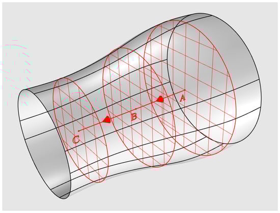
Figure 1.
Stream tube of ideal propulsor based on the momentum theory. Source: Authors based on [19].
This theory is based on the following assumptions:
- -
- The propulsor works in an ideal fluid without energy losses due to frictional drag.
- -
- The propulsor can be replaced in calculation cases by a theoretical actuator disc.
- -
- The propulsor is able to provide thrust without rotational effects on water flow.
Three typical cross sections are introduced to study the acceleration of the flow between the upstream and the downstream caused by the pressure jump of the actuator disc:
- -
- Station A—cross section located far upstream;
- -
- Station B—section in the plane of the actuator disc;
- -
- Station C—cross section located far downstream.
The power absorbed by the propulsor is given by:
It is also equal to:
The thrust generated by the propulsor is given by:
When examining fluid flow, the basic laws of physics can be applied, i.e., conservation law of mass, conservation law of momentum, and conservation law of energy. All these laws, as well as viscous phenomena in real (Newtonian) fluid, are reflected in the Navier–Stokes equations that describe both laminar and turbulent flow.
The Navier–Stokes partial differential equations are applicable for all unit actions on the fluid particle in three basic directions of space, i.e., weight, pressure, and friction and inertia. They can be simplified to the form:
These equations can be interpreted as the specific form of Newton’s second law for the flow of viscous incompressible fluid per unit mass, on the right with the product of acceleration and weight and on the left with the sum of mass and surface (pressure and viscous) forces [20,21].
The CFD method is the most commonly used in computer modeling of fluid flow. Several mesh-based methods have been developed in this area, where the geometry under investigation is replaced by a 2D or 3D mesh and the flow problem is solved using the Navier–Stokes equations (Figure 2). The basic principle of CFD is to create a computational domain that consists of a geometric model of the actual and discretized form (mesh), a definition of boundary conditions, a set of physical properties and calculation methods, and possibly external geometry boundaries of the flow area (external flow).
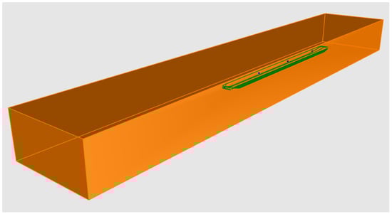
Figure 2.
3D geometry of a typical CFD domain (Layout E, deep water). Source: Authors.
In the CFD simulation of sailing, the geometry under investigation consists of the outer surface of the hull, surrounded by a flow area, mostly of hexahedral shape. This is a typical case of external flow where the flow takes place in the surrounding environment and not within the computational geometry. The investigated physical phenomena take place in a multiphase environment, at the boundary of two phases (water–air), which considerably increases the computational complexity of these tasks.
The most serious limitation in CFD analysis is the number of mesh elements (and nodes). In each iteration of the calculation, the hydrodynamic state of the elements is evaluated individually, and their excessive number can enormously increase computational complexity and machine time. For this reason, it is necessary to keep the number of elements as low as possible, but not to the detriment of the accuracy of the calculation.
We call it a quality mesh when the elements have the same size, are geometrically regular, and their distribution is also regular in the discretized area. A suitable choice of element size ensures that the hydrodynamic properties of the flow are captured, but velocities are decisive for dimensions [20,21].
Many numerical methods have been developed to address particular physical problems. Their application depends both on the suitability of the method for solving the issue and on the history of development.
By replacing the geometry of the examined area with a mesh of generated nodal points, the flow calculation domain is discretized, thus, allowing the flow equations to be converted into algebraic equations.
The finite volume method (FVM) is a method that, in a discretized form, retains very reliably the principles of conservation laws of balanced physical quantities in the control volume and is, therefore, the most widely used CFD simulation apparatus for solving the Navier–Stokes equations [22].
Numerical modeling of turbulent flows is still in the process of research and development, supported by the latest knowledge of mathematics, physics, and technical computational methods. However, there is no universal model of turbulence that is generally and effectively applicable in all cases. In order to choose the most suitable model for a particular calculation case, it is necessary to consider the possibilities and limitations of individual numerical models.
The time-averaging method (RANS—Reynolds-averaged Navier–Stokes equations), which has relatively low computational capacity requirements and provides acceptable accuracy, is becoming increasingly widespread in engineering simulations. It consists of parametric modeling of turbulent flow by time-averaged values of physical quantities using the Reynolds method. Several different RANS methods have been developed for various specific task types, which simplify the modeling of swirls using added transport equations [23].
For simulation purposes, a typical Danube cargo ship hull has been chosen with a pushed barge type bow (to be able to push barges) and with a simplified aftship suitable for all the examined layouts (Figure 3). The main particulars of the ship hull are shown in Table 1.
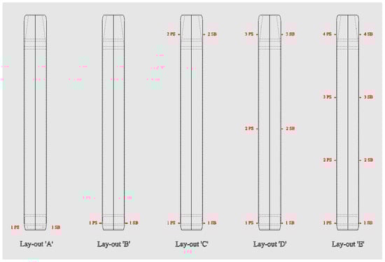
Figure 3.
Different hull/propulsion layouts examined by CFD analyses. Source: Authors.

Table 1.
Basic ship dimensions.
The dimensions of the hexahedral calculation domain are shown in Table 2.
Table 2.
Dimensions of the hexahedral calculation domain.
The layout cases of the CFD domains were designed as follows:
- -
- One-half (SB) of the ship hull and the surrounding environment is modeled.
- -
- Identical hull geometry is used for all the cases.
- -
- Uniform pressure jump dp = 100,000 Pa is applied for all the actuator discs.
- -
- Uniform total surface area (sum) of actuator discs is 1.2 m2 on one side.
- -
- Monitoring surfaces are assigned to every actuator disc on the upstream and the downstream sides with the same offset.
The CFD analyses have been performed with identical set-up parameters (Table 3). Only the boundary conditions and the initializing values vary from case to case.
Table 3.
CFD set-up parameters.
The following hull/propulsion layout cases have been analyzed for discrete flow speed values taken from the vessels working in the range 0–6 m/s:
- -
- A: Traditional 2 stern-mounted propulsors (twin-screw) layout (without tunnel and fins);
- -
- B: 2 side propulsion units mounted in the aft hull zone (symmetrically);
- -
- C: 4 side propulsion units mounted in the aft and fore hull zones (2 + 2, symmetrically);
- -
- D: 6 side propulsion units mounted in the aft, mid, and fore hull zones (2 + 2 + 2, symmetrically);
- -
- E: 8 side propulsion units mounted evenly along the ship hull (2 + 2 + 2 + 2, symmetrically).
The actuator disc was simulated using a fan boundary condition in the ANSYS Fluent CFD package. A boundary condition was applied on a circular surface whose diameter was set so that the total area of the propellers was constantly 2.4 m2. Diameters and locations of actuator disk centers in individual layouts are shown in Table 4.
Table 4.
Actuator disc parameters.
Special attention has been paid to cases C, D, and E because they can be considered as distributed ship propulsion systems, which were the main focus of interest.
For comparison reasons, all the studied cases have been examined under restricted draft conditions in shallow water, keeping a minimum of 0.3 m UKC, and also, under unrestricted draft conditions in deep water.
A total of 50 CFD flow analyses have been performed for unrestricted and restricted draft conditions. The mass flow rate values recorded for the actuator disc and the upstream/downstream monitors at every propulsion position have been used in Equation (4) of the Rankine momentum theory to obtain the increase in thrust generated by the propulsor. The power absorbed by the propulsors has been calculated by means of Equation (2) from the already known thrust value.
A visual check of the water flow field around the ship hull and the propulsors, the free surface of the water, and the wave pattern is possible in the graphical output generated by the CFD system (Figure 4). Some special variations in the values of the reported hydrodynamic quantities can be easier understood in this simple way (Figure 5).
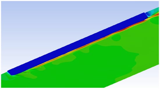
Figure 4.
Velocity magnitude on the free water surface (Layout E, deep water). Source: Authors.
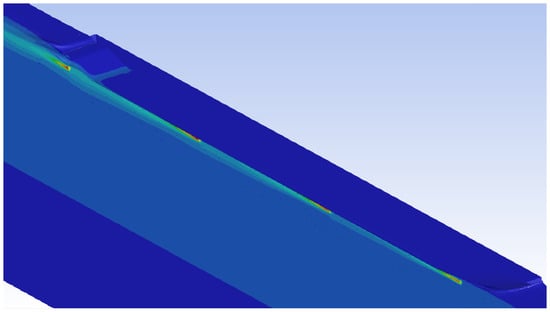
Figure 5.
Dynamic pressure at the propulsors’ center plane (Layout E, deep water). Source: Authors.
3. Results and Discussion
The resulting values of mass flow increase, generated thrust, and absorbed power are shown in Figure 6, Figure 7, Figure 8, Figure 9, Figure 10 and Figure 11, where their relative values are represented for an easier comparison and evaluation.
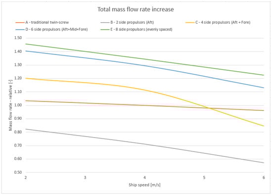
Figure 6.
Total mass flow rate, deep water (comparison). Source: Authors.
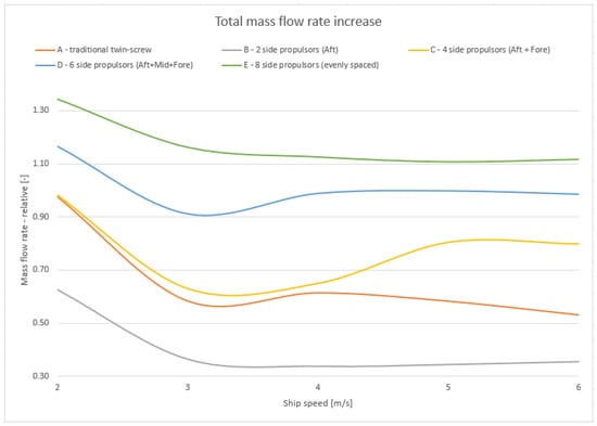
Figure 7.
Total mass flow rate, shallow water (comparison). Source: Authors.
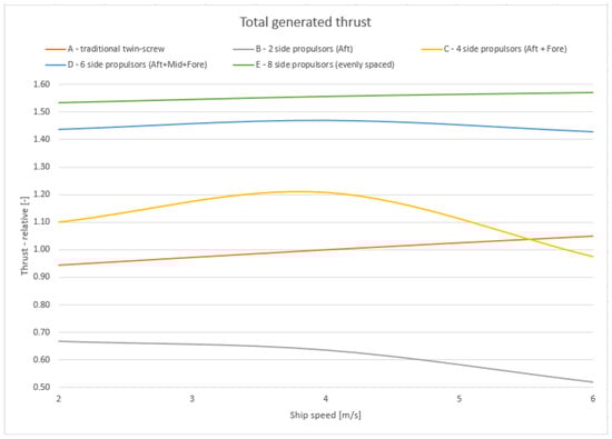
Figure 8.
Total generated thrust, deep water (comparison). Source: Authors.
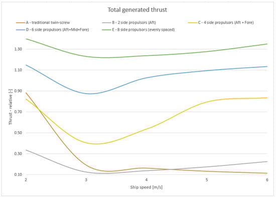
Figure 9.
Total generated thrust, shallow water (comparison). Source: Authors.
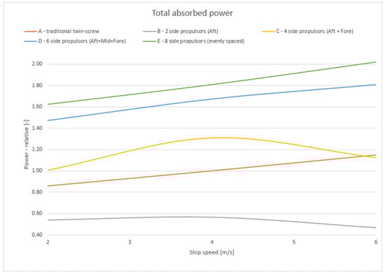
Figure 10.
Total absorbed power, deep water (comparison). Source: Authors.
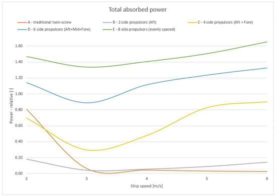
Figure 11.
Total absorbed power, shallow water (comparison). Source: Authors.
In the following comparative line graphs, the resulting total values are shown, where every curve represents a specific hull/propulsion layout. The absolute values of layout A in deep water at a mean speed of 4 m/s have been chosen as the reference unity values to calculate the relative values.
Rapid changes and some problematic areas can be identified easily in these graphs. In general, a significant fall in performance indicates intensive air intake into the propulsor. The occurrence of such ventilation can be checked visually in the graphical output from the CFD analysis.
In the figures showing the restricted water conditions, a special region can be localized around the sailing speed of 3 m/s. All the curves have a “wave trough” at this area, and this is a hot candidate for a speed value characteristic for this specific hull and water flow field.
It can also be seen that the absence of the propulsion tunnel (and fins) has a much more significant impact on the performance of hull/propulsion layout A (traditional twin-screw) under the restricted sailing conditions.
To show which propulsion locations are prone to have a strong air intake from the free water surface, a different type of figure has been introduced.
The examples in Figure 12 and Figure 13 represent the resulting generated trust and absorbed power values for hull/propulsor layout E (8 propulsors) on a per-propulsor basis. For these two special graphs, the absolute values of the aftmost propulsor at speed 2 m/s in shallow water have been chosen as the reference unity values.
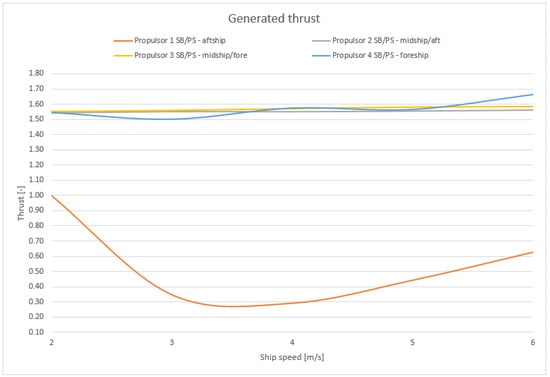
Figure 12.
Propulsion thrust, shallow water (layout E). Source: Authors.
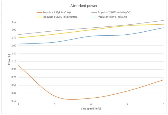
Figure 13.
Propulsion power, shallow water (layout E). Source: Authors.
In this example case, the critical propulsor position is No. 1, which is located in the aftship zone of the hull (aftmost side propulsors, see Figure 14). Intensive ventilation of the propulsion is typical for this location also in other layouts. The performance of propulsor No. 4, located in the foreship zone (foremost side propulsors), seems to be quite unstable; in some layouts, air intake is also present.
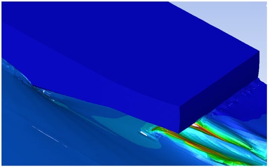
Figure 14.
View of the aftship air intake zone (Layout A, shallow water). Source: Authors.
Both propulsion positions are typically located at the curved (shaped) hull endings, where the water flow speeds up quickly, causing a pressure drop and a wave trough. Therefore, the air intake occurs much easier in these locations than in the straight and long midship area.
The following comparative figures (Figure 15 and Figure 16) show the thrust and power curves of three distributed propulsion layouts (C, D, E) in restricted and unrestricted water depth conditions. The thrust and power of layout A at mean speed 4 m/s in deep water have been used as unity values.
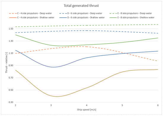
Figure 15.
Thrust of distributed systems in deep and shallow water conditions. Source: Authors.
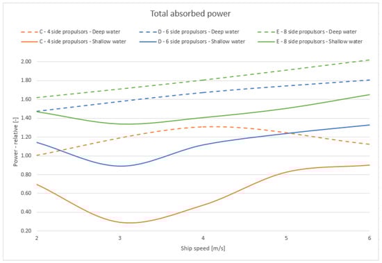
Figure 16.
Power of distributed systems in deep and shallow water conditions. Source: Authors.
Generally, after comparing the hydrodynamical performance in Figure 6, Figure 7, Figure 8, Figure 9, Figure 10, Figure 11, Figure 15 and Figure 16 of ideal propulsors under both water depth conditions, it can be stated that the distributed propulsion systems consisting of 4+ (preferably 6 or 8 or more) units produce noticeably higher thrust effects in shallow water sailing than the traditional aft end layouts. Under restricted conditions, the thrust increase between two distributed layouts with a different number of propulsors is higher in contrast to deep water sailing, where differences in performance are not so significant.
The aim of this investigation was not to evaluate the absolute values of hydrodynamic quantities obtained from CFD analyses, but rather, to find new ways and possible principal solutions for shallow water propulsion systems. Due to the large number of CFD simulations to be performed, some simplifications had to be made on the computational domain in order to keep the computing time at a reasonable level. For the same reasons, the real propulsion units have been represented with ideal propulsors (actuator discs).
However, the accuracy reached in this way by CFD calculations is sufficient only if the relative quantity values are needed for comparison purposes. The resulting main performance parameters of all the examined propulsion layouts have been compared properly, so it was possible to filter out the most promising solutions. The comparison of the results from the restricted and unrestricted water depth conditions has clearly shown the differences in the courses of their graphs.
To determine the effect of mesh quality, a dependence study has been performed for case E in shallow water. For the new analyses, the CFD mesh of the entire computational domain has been refined by halving the average element sizes. With these several times larger amounts of elements, the interval of sailing speeds from 2 to 6 m/s has been analyzed and the results have been compared with the values obtained from the original coarser mesh. The result of this comparison is shown in Figure 17 as percentage difference of the new values from the reference values. The graph shows that in the operating range of the vessel, the maximum difference value is close to 2.5%, which is fully acceptable for comparison purposes.
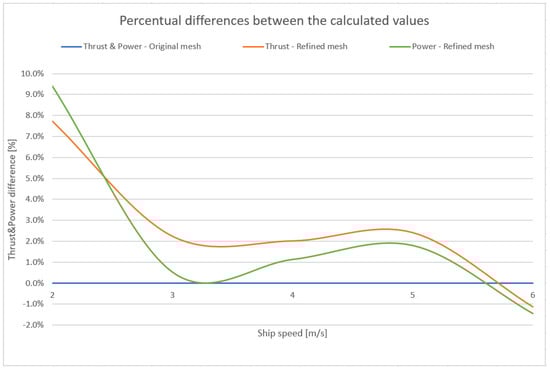
Figure 17.
Percentual comparison of the original and the refined mesh results. Source: Authors.
In the technical literature, the expressions “distributed propulsion system” or “multiple propeller ship” refer to ships which are equipped with more than three propulsors (propellers) in general, located in the aftship area and arranged in different geometric patterns. Based on the lack of available publications concerning side-mounted propulsions, it can be assumed that we have given a new meaning to the expression “distributed propulsion”.
Similar R&D and experiments have been performed in the past for another reason, i.e., for better longitudinal distribution of thrust power in terms of the propeller load and cavitation. The best-known cases are overlapping propellers and tandem propellers (their modern versions are twin propeller azimuths and pods), which have also been implemented on experimental ships. Overlapping propellers each have their own shaft line, while the tandem system is mounted on a single common shaft. However, all these propulsions are located in a traditional place under the stern part of the ship (aft end layout), which is a significant difference from the distribution along the side of the ship that we have investigated. In addition, these systems tend to appear as integrated propulsion units due to their small distance from each other. Based on the significant differences and the poor documentation of the above listed cases, they have not been mentioned in the work as reference cases or comparative bases.
For a final validation of the working method, it was not possible to make a comparison of our CFD-based results with other published results from earlier investigations either made by computer simulations or by model tests made in towing tanks. No usable publication reporting a similar approach studying longitudinal distribution of propulsion units has been found up to now.
4. Conclusions
The analysis results have confirmed that shallow water vessels driven by distributed (side-mounted) propulsion systems can be operated efficiently, eliminating the unwelcome side effects of the traditional stern-mounted propeller systems. The preliminary assumptions have been substantiated, at least at the simulation level.
Technical implementation of the propulsors was beyond the scope of this work. Standard propeller-based propulsion units are probably not usable because of their tendency to take in the air from near the free water surface. Rather, different, more suitable propulsors should be employed, or a completely new concept should be developed for this special purpose.
This was the first step of investigations around distributed propulsion systems, bringing purely principal solutions to the problem. In the next step, the most promising hull/propulsion layouts should be further examined at a higher level by performing a series of complex and demanding CFD analyses. The most appropriate are layouts E and D (8 and 6 units), but for shorter ship hulls, layout C (4 units) could be useful as well. In this phase, a new side-mounted type of propulsion unit should be preliminarily designed. The purpose of the third phase should be the validation of the results from the previous two phases. Preferably, a towing tank test should be performed, examining the real hull-propulsion interactions.
The main contribution of this work is that it shows a possible way how the more efficient vessels of the future intended for restricted navigation depth could be developed. Such vessels could also operate on waterways where the ships with a traditional hull and propulsion can no longer do so, either for technical or economic reasons. Further R&D tasks should lead to the development of special propulsors and hulls optimized for their best interaction in restricted but also in unrestricted conditions of navigation.
Author Contributions
Conceptualization, L.I., T.K. and M.J.; methodology, L.I. and M.J.; software, L.I.; validation, L.I., T.K. and M.J.; formal analysis, M.J.; investigation, L.I., T.K., M.J. and V.L.; resources, M.J. and V.L.; data curation, T.K.; writing—original draft preparation, L.I.; writing—review and editing, M.J.; visualization, T.K. and V.L.; supervision, T.K. and M.J.; project administration, T.K and M.J.; funding acquisition, T.K. and M.J. All authors have read and agreed to the published version of the manuscript.
Funding
This research was funded by Institutional research of the Grant system of the Faculty of Operation and Economics of Transport and Communications, University of Zilina. This research is also the result of the Project VEGA No. 1/0128/20: Research on the Economic Efficiency of Variant Transport Modes in the Car Transport in the Slovak Republic with Emphasis on Sustainability and Environmental Impact, Faculty of Operation and Economics of Transport and Communications, University of Zilina, 2020–2022.
Conflicts of Interest
The authors declare no conflict of interest.
References
- David, A.; Madudova, E. The Danube river and its importance on the Danube countries in cargo transport. In Proceedings of the 13th International Scientific Conference on Sustainable, Modern and Safe Transport, TRANSCOM 2019, High Tatras, Slovakia, 29–31 May 2019. [Google Scholar]
- Danube River Basin Climate Change Adaptation, Final Report. Department of Geography, Chair of Geography and Geographical Remote Sensing, Ludwig-Maximilians-Univesitat Munich, Germany. 2018. Available online: https://www.icpdr.org/main/sites/default/files/nodes/documents/danube_climate_adaptation_study_2018.pdf (accessed on 15 June 2020).
- Alberto, P.; Hylke, B.; Bernard, B.; Emiliano, G.; Carlo, L.; Janos, F. Water scenarios for the Danube River Basin: Elements for the assessment of the Danube agriculture-energy-water nexus. JRC Tech. Rep. 2016. [Google Scholar] [CrossRef]
- Stopka, O.; Simkova, I.; Konecny, V. The quality of service in the public transport and shipping industry. Nase More 2015, 62, 126–130. [Google Scholar] [CrossRef]
- Buchler, D.; Luck, R.; Markert, M. Propulsion and control system for shallow water ships based on surface cutting double Propellers. In Proceedings of the 8th IFAC Conference on Control Applications in Marine Systems, Rostock-Warnemunde, Germany, 15–17 September 2010. [Google Scholar]
- Raven, H. A new correction procedure for shallow-water effects in ship speed trials. In Proceedings of the 13th International Symposium on PRActical Design of Ships and Other Floating Structures PRADS’ 2016, Copenhagen, Denmark, 4–8 September 2016. [Google Scholar]
- Rotteveel, E.; Hekkenberg, R.; Ploeg, A. Inland ship stern optimization in shallow water. Ocean. Eng. 2017, 141, 555–569. [Google Scholar] [CrossRef]
- Schlichting, O. Schiffwiderstand auf beschränkter wassertiefe: Widerstand von seeschiffen auf flachem wasser. Jahrb. Schiffbautech. Ges. 1934, 35, 127. [Google Scholar]
- Lackenby, H. The effect of shallow water on ship speed. Shipbuild. Mar. Eng. 1963, 70, 446–450. [Google Scholar]
- Tuck, E. Hydrodynamic problems of ships in restricted waters. Annu. Rev. Fluid Mech. 1978, 10, 33–46. [Google Scholar] [CrossRef]
- Ferreiro, L.D. The effects of confined water operations on ship performance: A guide for the perplexed. Nav. Eng. J. 1992, 104, 69–83. [Google Scholar] [CrossRef]
- Rotteveel, E.; Hekkenberg, R. The influence of shallow water and hull form variations on inland ship resistance. In Proceedings of the 12th International Marine Design Conference (IMDC), Tokyo, Japan, 11–14 May 2015. [Google Scholar]
- Raven, H. A computational study of shallow-water effects on ship viscous resistance. In Proceedings of the 29th Symposium on Naval Hydrodynamics, Gothenburg, Sweden, 26–31 August 2012. [Google Scholar]
- Harvald, S.A. Wake and thrust deduction at extreme propeller loadings for a ship running in shallow water. RINA Suppl. Pap. 1977, 119, 20–21. [Google Scholar]
- Zhao, L. Optimal ship forms for minimum total resistance in shallow water. Schriftenreihe Schiffbau 1984, 445. [Google Scholar] [CrossRef]
- Saha, G.K.; Suzuki, K.; Kai, H. Hydrodynamic optimization of ship hull forms in shallow water. J. Mar. Sci. Technol. 2004, 9, 51–62. [Google Scholar] [CrossRef]
- Galierikova, A.; Sosedova, J. Environmental aspects of transport in the context of development of inland navigation. Ekol. Bratisl. 2016, 35, 279–288. [Google Scholar] [CrossRef]
- Sugalski, K.; Skrucany, T. Grid type impact on the results of the volume of fluid method in the free surface flow calculations around ship hull. In New Trends in Production Engineering; De Gruyter: Warsaw, Poland, 2018; Volume 1, pp. 151–157. [Google Scholar]
- Carlton, J. Marine Propellers and Propulsion, 4th ed.; Butterworth-Heinemann: Oxford, UK, 2019. [Google Scholar]
- Ganco, M. Fluid Mechanics; ALFA: Bratislava, Slovakia, 1983. [Google Scholar]
- Douglas, J.F.; Gasiore, J.M.; Swaffield, J.A.; Jack, L.B. Fluid Mechanics, 5th ed.; Pearson: Harlow, UK, 2005. [Google Scholar]
- Molnar, V. Computational Fluid Dynamics—Interdisciplinary Approach with CFD; University of Technology in Bratislava (STU): Bratislava, Slovakia, 2011. [Google Scholar]
- Kudelas, D. Basic of Computer Flow Modelling and Visualization; Faculty of Mining, Ecology, Process Control and Geotechnologies: Kosice, Slovakia, 2017. [Google Scholar]


© 2020 by the authors. Licensee MDPI, Basel, Switzerland. This article is an open access article distributed under the terms and conditions of the Creative Commons Attribution (CC BY) license (http://creativecommons.org/licenses/by/4.0/).