Hydrodynamic Measurements of Propagating Waves at Different Nearshore Depths in Hujeong Beach, Korea

Abstract

This paper reports the results of hydrodynamic measurements at two different water depths to observe wave properties in the course of wave propagation, especially during storm periods, in Hujeong Beach, Korea. In addition to hydrodynamic measurements, video monitoring data and satellite images from Sentinel-II were employed to compare the temporal changes in shoreline positions and shallow water bathymetry during the storms. Through combination of a variety of observational data sets, the accuracy of analysis could be enhanced by preventing possible misinterpretation. Two significant storms were observed from two experiments conducted at different times and locations of the beach. The hydrodynamic conditions were similar in both of the periods in terms of wave and current conditions as well as wave nonlinearity such as skewness. However, the response of shoreline during the two storms was the opposite because it was eroded during the first storm but advanced during the second storm. This suggests that other controlling factors such as storm duration need to be investigated to support the analysis of cross-shore sediment transport and consequent shoreline evolution for future studies.

1. Introduction

Coastal erosion is a critical issue as it may cause impacts on human life when the sand in recreational beaches or sediments used to protect coastal facilities are lost permanently. The retreat or accretion process of the shorelines is a result of coastal sediment transport that occurs mainly in the surf zone where the wave energy is transferred to kinetic energy due to wave breaking. There are two modes of sediment transport according to the direction of their motions—longshore and cross-shore sediment transport. When the waves are obliquely incident, the momentum of breaking waves generates shore-parallel radiation stresses that produce longshore current and the consequent longshore sediment transport. Therefore, the direction of longshore transport corresponds to that of the wave incidence, which can be predicted without difficulty. The cross-shore transport refers to the motions of sediments perpendicular to the shoreline due to waves, currents, and their combined motions. Unlike the longshore transport, the direction of cross-shore transport is not easily predictable as it depends on a variety of wave and current conditions that are difficult to be precisely measured. In general, sediments move offshore under energetic wave conditions causing sediment erosions from the shore, which occurs in short time period during such as storm events [1,2]. Onshore sediment motion prevails under mild wave conditions and it occurs over relatively longer periods at the month scale [2,3]. The net cross-shore sediment transport is the result of a balance between these onshore- and offshore-directed components, and thus an accurate description of them is important in predicting the dynamic evolution of beach profiles [4].

The nonlinearity of shoaling waves have been commonly studied using numerical models (e.g., [3,5,6,7,8]) and/or lab experiments (e.g., [9,10]). For example, new formulations for seabed shear stress, a fundamental component to calculate sediment transport, have been developed by incorporating $S_k$ and $A_s$ using model [11] and lab data [9]. Although it is not easy to observe the nonlinear wave shape parameters in the field where wave irregularity prevails, data measured with wave gauges have been applied to elucidate the nonlinear wave dynamics in various ways. From the measurements of shoaling surface gravity waves, $S_k$ and $A_s$ were estimated as the real and imaginary parts of bispectra respectively [12]. The bispectral analysis was also applied to investigate the spatial variation of $S_k$ and $A_s$ of orbital velocities for shoaling and breaking waves in terms of Ursell parameter [13]. Since $S_k$ and $A_s$ vary as waves propagate over the shoaling area, it is important to understand their spatial variation along the propagation path. Using an array of flow meter across a surf zone, velocity acceleration field was observed to be strongly skewed in the shoreward direction [14]. In addition, hydrodynamic measurements along cross-shore profiles were used to develop empirical formulations to describe wave nonlinearity in terms of depth and other wave parameters [4]. The impact of velocity skewness on the sediment transport was investigated in terms of the seabed ripple movement to observe that the wave spectra in the storm growing/decaying phase were closely related with the signs of $S_k$ and the direction of ripple migration [15,16]. In the offshore outside the surf zone, laser altimeters could be applied to measure the wave asymmetry and steepness [17]. Recently, the impact of seabed roughness on the wave transformation was studied by measuring $S_k$ and $A_s$ over rocky platforms where the wave energy was dissipated [18].

In the present study, we measured the hydrodynamics and wave nonlinearity at two different depths of a field site to examine the spatial changes by the shoaling and breaking during wave propagation under various wave conditions. Previously, we observed a rapid seabed erosion at a water depth of 8–9 m during an extreme wave condition over an approximately two-day period in Hujeong Beach [19]. This paper contains the results from follow-up studies with additional data sets measured at different locations and times in order to mainly examine the spatial variation of wave parameters under such extreme conditions as well as normal wave conditions. In addition to the hydrodynamic measurements, we employed two additional data sets. First, the shoreline data obtained from a video monitoring system (VMS) installed in the middle of the experimental site were analyzed in the corresponding experimental period. The VMS provides the beach width calculated from the shoreline positions averaged over 10 min video data, which have been usefully applied to understand the characteristic process in the Hujeong Beach [20]. In addition, Sentinel-II satellite images were employed to observe nearshore morphology that supported the results from the hydrodynamic data. Recently, the Sentinel satellite data with high spatial resolution and short orbital cycle were used to detect nearshore sandbar in shallow coastal waters [21]. We also used the satellite images to show their movement in accordance with the wave measurements. The purpose of this study is then to examine the coastal processes associated with cross-shore sediment movement in terms of the wave nonlinearity in various wave conditions, using on-site and remotely sensed measurements.

2. Materials and Methods

2.1. Field Experiments

In this study, we used two data sets measured at December 2016–January 2017 and at December 2018–January 2019 in Hujeong Beach, east coast of Korea (Figure 1a). At Hujeong Beach, the East Sea Research Institute (ESRI) of Korea Institute of Ocean Science and Technology (KIOST) is located. The Hujeong Beach is a micro-tidal area where the tidal range is ~0.2 m. The wave climate is moderate as the average wave height is usually not higher than 1.0 m. During winter, however, severe storm waves frequently attack the site from the northeast with waves higher than 4 m. In addition, this area is influenced by typhoons occasionally in summer. The sediment size in the nearshore area of the beach is coarse sand as ~0.5 mm. The beach is vulnerable to erosion since the construction of Hanul nuclear power plant in the north of the beach [19,20]. Figure 1b shows an aerial photo over the Hujeong Beach in 1980 when the beach was in equilibrium before the construction of the power plant. One of the missions of ESRI is to perform studies on coastal processes including measurements of seabed bathymetry using echosounders as the beach is characterized with its pocket shape and nearshore crescentic sandbars as shown in Figure 1c. As one of the outcomes, an unexpected severe erosion of seabed was observed by deploying a set of instruments in the depth of ~8 m [19].

In this study, parts of data from [19] have been used to estimate wave and current properties at the same location (designated as L1 for this study). The hydrodynamic data were also measured at shallower depth (L2) using a set of acoustic instruments during the same period, which were able to compare with the data for propagating waves. Figure 1c shows the two locations of the deployed instruments of L1 and L2 of the experiment during December 2016 and January 2017 (hereafter, Exp#1). The water depths measured at the initial time of deployment were 8.1 m and 3.3 m at L1 and L2 respectively. Detailed specification of the measured data during Exp#1 is listed in

Table 1. Specification of measurements ate L1 and L2 during Exp#1.

	L1	L2
Location (Lat, Lon)	37°04′45.82″ N	37°04′42.49″ N
	129°24′28.32″ E	129°24′14.10″ E
Water depth	8.1 m	3.3 m
Instruments	VECTOR (Nortek), ADCP (RD Instruments)	ADV (SonTek)
Measurement height above seabed	0.25 m
Time for t = 0 (day)	20 December 2016 11:00
Measurement burst interval	60 min
Sampling frequency	2 Hz
Burst duration	20 min
Data points in one burst	2400

. Another field experiment was performed ~2 years later from Exp#1 at the similar locations of the Hujeong Beach in December 2018 and January 2019 (hereafter, Exp#2). The locations of two measurements (L3 and L4) during Exp#2 are also marked in Figure 1c, and its specification is listed in

Table 2. Specification of measurements ate L3 and L4 during Exp#2.

	L3	L4
Location (Lat, Lon)	37°04′42.90″ N	37°04′38.19″ N
	129°24′27.39″ E	129°24′22.22″ E
Water depth	5.5 m	3.5 m
Instruments	VECTOR, Signature 500 (Nortek)	ADV (SonTek)
Measurement height above seabed	0.25 m
Time for t = 0 (day)	21 December 2018 07:00
Measurement burst interval	60 min
Sampling frequency	4 Hz
Burst duration	10 min
Data points in one burst	2400

. Unfortunately, the instruments in L4 were buried under ground at 29 December 2018 and thus L4 data were not available after that. Since the purpose of this paper is to compare the difference of hydrodynamics of propagating waves at two locations of different depths, the damage on the measurement in L4 prevented further analysis regardless of the data availability in L3 for a longer period.

The measured flow data were processed to calculate representative values for each burst. First, the velocities were decomposed into the cross-shore and longshore directions as $+u$ indicated the onshore direction and $+v$ directed to the left of the shore shown in Figure 1. Due to the contamination on the raw data by acoustic instruments, especially for those moored at shallower depths in L2 and L4, despiking and filtering were necessary to exclude the unordinary data for the analysis. When the number of despiked data exceeded 20% of the whole data in the burst, the analysis was not performed, and the representative values of that burst were not estimated because of the high possibility of data contamination. For this reason, the analyzed data are available only for t = 2–18 and 24–32 for Exp#1 (time was set 0 at 20 December 2016 for Exp#1). For Exp#2, the instruments in L4 were buried under ground since t = 7 (time was set 0 at December 21, 2018 for Exp#2) and its data were only available for t = 0–7 for Exp#2. The three periods with valid data in both Exp#1 and Exp#2 are set as T1, T2 and T3 respectively. In addition, there were times when data were not available even during T1–T3 when the despiked and filtered data were still contaminated. For example, the data in t = 6–8 were not available in T1. From the flow measurements, five parameters were estimated based on the horizontal velocity components. The velocity magnitude was defined as $V_{mag}=\overline{\sqrt{u{\left(t\right)}^2+v{\left(t\right)}^2}}$, and the mean velocity components were calculated as $\overline{u}=\overline{u\left(x\right)}$ and $\overline{v}=\overline{v\left(x\right)}$. The skewness was estimated from the cross-shore velocity component as $S_k=\raisebox{1ex}{$\overline{u{\left(t\right)}^3}$}\!\left/ \!\raisebox{-1ex}{$\overline{u{\left(t\right)}^2{}^{3/2}}$}\right.$ and asymmetry was computed as $A_s=\raisebox{1ex}{$\overline{H{\left[u\left(t\right)\right]}^3}$}\!\left/ \!\raisebox{-1ex}{$\overline{u{\left(t\right)}^2{}^{3/2}}$}\right.$ where $H$ is the Hilbert transform [22].

2.2. Video Monitoring System

VMS images have been usefully applied for decades to monitor long-term beach process [23]. Recently, new VMS methodologies such as surf cameras have been developed to provide more efficient ways for shoreline data collection [23,24]. In this study, a conventional VMS was used as it was constructed on the top of 30 m-high monitoring tower in the middle of Hujeong Beach on 9 December 2016, 11 days before the field measurements for Exp#1 started. The VMS data have been usefully employed to understand shoreline processes of the ~2.4 km long beach by using eight video cameras [20]. The VMS provides shoreline positions per hour on a clear day during the daytime, which have been used to calculate the beach area outside the water. Under harsh wave conditions, the shoreline data cannot be obtained due to the contamination of wave breaking that makes the shoreline positions blurred. The images taken by each video camera were combined into a 2-D image. In this process, the angle of each camera was considered to calibrate the tilted image to the vertical line. After that, 600 snapshot images were averaged for 10 min per hour to remove the noise produced by wave breaking, and the shoreline positions were extracted manually, providing metric measurements of shoreline data.

In Figure 2, the shoreline data measured from the VMS on 19 December 2016 and 29 December 2016 are compared. It shows that the shoreline was not straight along the beach, but had undulations as there were several locations where the shoreline was protruded to the sea. These protrusions were likely related to the nearshore sandbars that were observed at 3–5 m water depth [20]. In this study, the shoreline positions will be compared at different times to understand the beach process during the experimental period.

2.3. Sentinel-II Satellite Images

An additional dataset was obtained from the satellite images. Sentinel-II is an Earth observation mission to acquire optical imagery over land and coastal waters with high spatial resolution (10 m to 60 m), developed and operated by European Space Agency since 2015 [25]. Figure 3 shows a sentinel-II image taken over the experimental site of Hujeong Beach on 11 December 2016, downloaded from Creodias (creodias.eu), a platform that provides Sentinel-II images for free. It shows that the shorelines and the wave breaking lines are clearly captured in the image. Owing to the high spatial resolution (~10 m), the crescentic sandbars larger than 100 m can be detected, which provides big advantage to apply the Sentinel-II data in the nearshore studies. Moreover, the shortest revisit cycle of the Sentinel-II is 5 days by employing two identical satellites (Sentinel-IIA and IIB) as each of them has 10-day revisit cycle. Therefore, changes in the coastal features with months are measurable using the satellite data, if weather condition permits. The shoreline feature in Figure 3 confirms the shoreline positions measured by VMS in Figure 2. The shoreline was not straight but protruded at several locations along the shore. In addition, though it is not distinct, the features of crescentic sandbars can be seen in the shallow area of the water. Specifically, the horns of the sandbars are connected to the protruded locations in the shoreline showing an example of out-of-phase coupling [26].

3. Results

3.1. Wave and Hydrodynamic Measurements

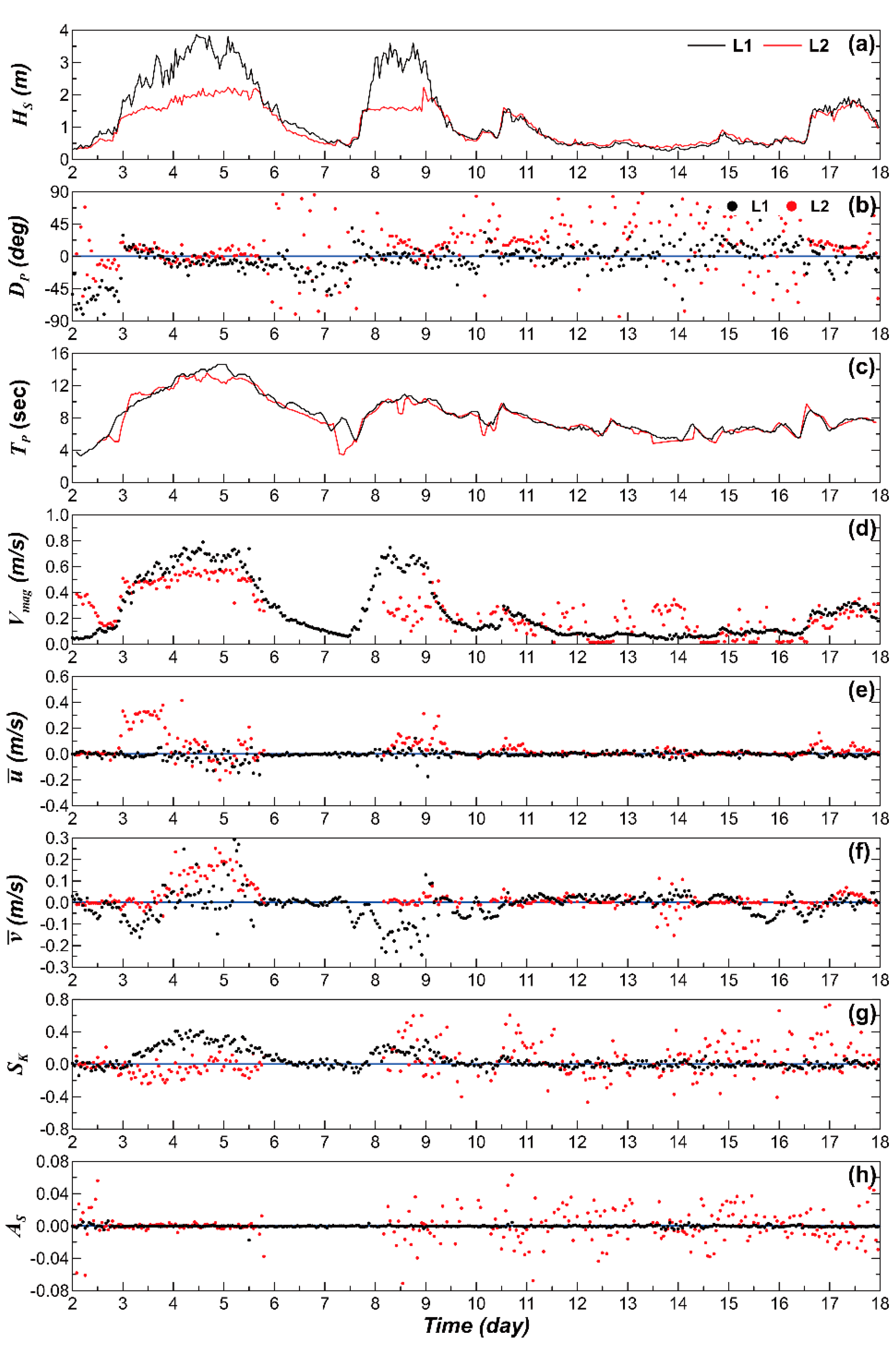
In panels a–c of Figure 4, Figure 5 and Figure 6, three wave parameters—significant wave height ($H_s$), Peak wave period ($T_p$), and peak wave direction ($D_p$)—are plotted for selected periods (T1, T2 and T3) of Exp#1 and Exp#2. The wave parameters were estimated based on the wave spectra calculated from the burst data, which gave averaged value per burst. The time is set zero at December 20, 2016 for Exp#1 and Figure 4 shows the time variation of the wave data for T1. In this period, the data in L1 are characterized with the distinctive periods of storm waves (Figure 4). Three extreme events (t = 3–6, 8–10) with $H_s$ > 3 m in L1 were clearly identified. The wave period also varied similarly with the wave height as it increased with increasing height. Specifically, $T_p$ became maximum reaching to 15 s at t = 5–6, corresponding to the high $H_s$ in this time. The wave propagation direction shows different pattern as the waves generally approached the shore in the normal direction ($D_p$ = 0) during the storm periods except for the sharp changes in t = 2–3. In Figure 5, the same wave data are plotted for T2 during which another storm wave attacked the beach with $H_s$ > 3 for longer time (t = 26–30) with wave periods of ~10 s and with nearly normal wave direction. For Exp#2, the initial time was set at 21 December 2018, and Figure 6 shows the three wave parameters for T3. In L3, the wave condition was less distinctive compared to that in L1 of Exp#1 as $H_s$ was significantly lower than those in L1, indicating that the wave condition was milder during Exp#2, and storm wave events in which $H_s$ exceeded 2 m over a period longer than 1 day did not occur (Figure 6a).

In Figure 4, the temporal variations of the five parameters during T1 of Exp#1 are compared between L1 and L2. As shown in Figure 4d, $V_{mag}$ sharply increased during the two storm periods in t = 3–6 and 8–9 in both locations, but $V_{mag}$ in L2 was lower than that in L1 likely because the wave orbital velocity magnitude decreased with decreasing water depth. It might be also because the wave energy in L3 decreased due to the wave breaking in L2, though there was no clear indication of the breaking during these storms. It should be noted that $\overline{u}$ in L2 sharply increased at t = 3–4 in the early stage of the first storm when $\overline{u}$ remained close to zero in L2 (Figure 4e), which indicates that strong onshore current developed in L2 when the storm developed. In L1, the onshore current was not observed. Instead, longshore current developed to the right of the beach at t = 3 (Figure 4f). Once the storm was fully developed at t = 4–5, the direction of the current in L1 rapidly changed as it $\overline{u}$ became negative and $\overline{v}$ changed to positive, showing that the current flowed offshore to the left of the beach. It should be also noted that $S_k$ of cross-shore velocity shows opposite pattern between L1 and L2 as it became positive in L1 but negative in L2 (Figure 4g). As analyzed in the previous study [19], the high positive $S_k$ in L1 likely increased the bed stress to cause the seabed erosion in this time. The negative $S_k$ in L2 could be understood that the wave steepness increased at L1 due to shoaling of storm waves decreased by wave breaking when they reached to L2. Contrary to the significant changes in $S_k$, $A_s$ remained close to zero in both L1 and L2. This low magnitude in $A_s$ during extreme wave condition was not clearly understood as the wave asymmetry usually increases under breaking wave condition (Figure 4h).

Once the storm period ended at t = ~6, the statistics of data in L2 was not available due to contamination until t = ~8 when the second storm waves occurred for shorter time period until t = ~9. The flow pattern was different from that in the first storm as $V_{mag}$ in L2 was lower during this second storm period while $V_{mag}$ in L1 was similar between them (Figure 4d). The direction of the cross-shore current was also different as $\overline{u}$ in L2 directed onshore. The most significant difference can be found in $S_k$ as it remained positive not only in L2 but also in L1, which indicates that the wave shoaling might be dominant instead of breaking in both locations (Figure 4g). In addition, $A_s$ shows clear difference between L1 and L2 at t = 8–9 as the magnitude of $A_s$ increased in L2 as it was dispersed in wider range, compared to that in L2 where $A_s$ remained close to zero similarly to that observed in t = 3–5 (Figure 4h). Since the positive/negative sign of $A_s$ means that the waves were tilted backward/forward [27], the higher $A_s$ during the second storm indicates that the waves were deformed when they approached from L1 to L2. Another period examined in Figure 4d is t = 12–18 when the wave energy became low after the storms. $V_{mag}$ in L2 shows more severe fluctuations compared to that in L1. It should be also noted that both $S_k$ and $A_s$ in L2 show higher dispersion around zero that led to their higher magnitude compared to those in L1 (Figure 4g,h). Specifically, $S_k$ in L2 tended to be positive, indicating that the waves became steeper as they approached the shore from L1. For $A_s$, this tendency was not found as negative values were also observed, showing that the waves were tilted but not necessarily forward.

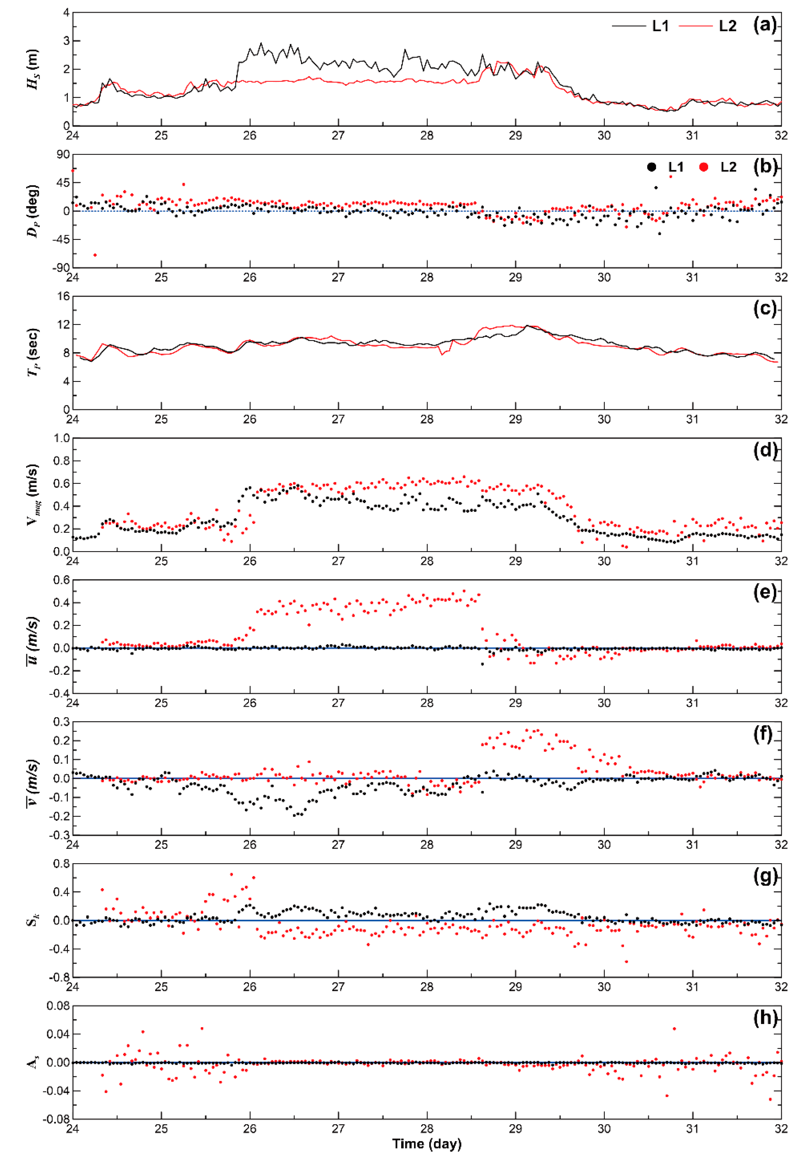
In Figure 5, the same five parameters are plotted but for t = 24–32 (T2) during which the third storm had lower $H_s$ compared to the previous two storms developed for longer period (t = 26–29). In this storm period, $V_{mag}$ increased to ~0.5 m/s in both L1 and L2. Interestingly, a strong onshore current was observed in L2 while no cross-shore currents were detected in L1 as $\overline{u}$ ~ 0 during the storm period. Difference between L1 and L2 was also observed in the longshore current as $\overline{v}$ = −0.2 m/s in L1 at t = 26 but $\overline{v}$ ~ 0 m/s in L2 at the same time. On the contrary, $\overline{v}$ ~ 0 m/s in L1 at t = 29 while it increased to ~0.2 m/s in L2. Except for the storm period, $\overline{u}$ and $\overline{v}$ were close to zero in both L1 and L2. As for the skewness, $S_k$ slightly increased in L1 during the storm as its maximum value reached to ~0.25 at t = 26 while $S_k$~0 before and after the storm period. In L2, $S_k$ sharply increased to ~0.5 just before the storm at t = 25–26. During the storm period, however, it became negative as it ranged between −0.1 and −0.2 at t = 26–29. Therefore, the pattern of positive skewness in L1 and negative skewness in L2 observed in the first storm (t = 3–5) repeated in the third storm even though its magnitude was lower. Except for the storm period, $S_k$ was remained close to zero in L1 but it was dispersed around zero in L2, increasing its magnitude, as also shown in Figure 4. The dispersion in L1 outside the storm period was more clearly observed in the wave asymmetry. During the storm period, $A_s$ was close to zero in both L1 and L2, which was similarly observed during the first storm (t = 3–6 in Figure 4). Except for the storm, however, $A_s$ was strongly dispersed and its magnitude increased in L2 while it remained close to zero in L1.

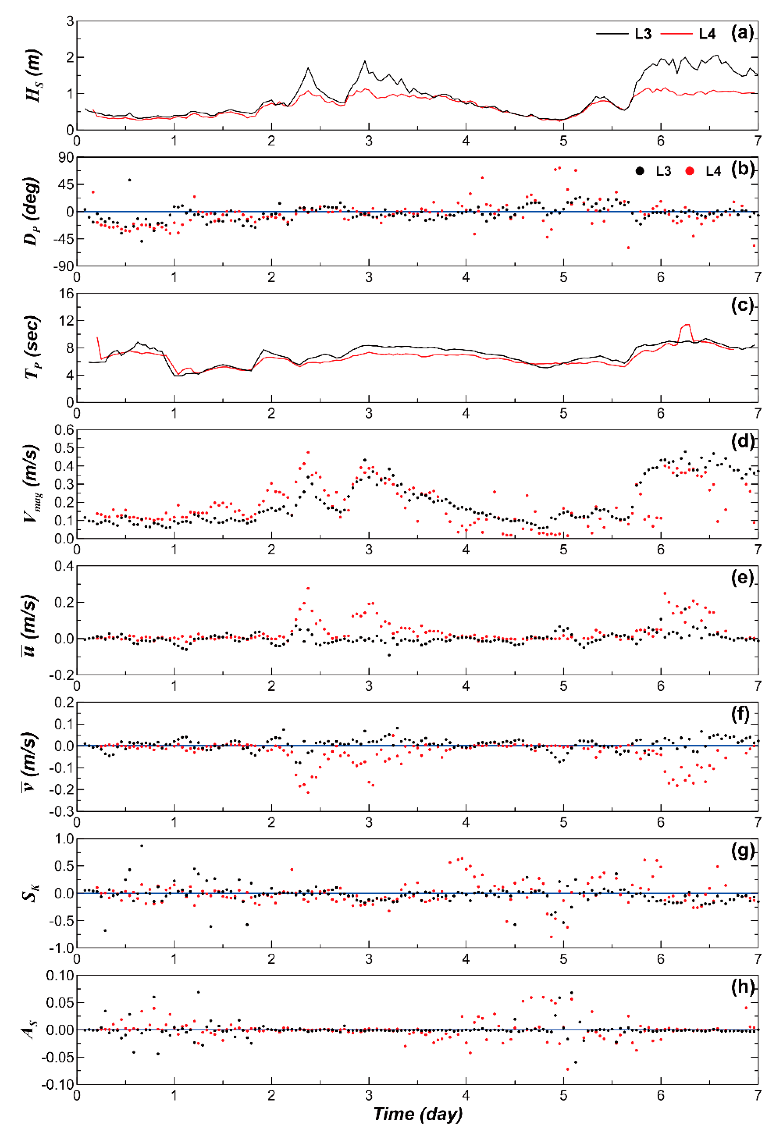
The characteristic pattern of $A_s$ is also clearly observed in Exp#2 as shown in Figure 6 in which the five hydrodynamic parameters are compared for T3 (December 21–28, 2018). In this time, a period of high waves when $H_s$ reached ~2 m was observed at t = 2–3 (Figure 6a). Correspondingly, $V_{mag}$ increased to reach ~0.5 m/s in both L3 and L4. In case of currents, however, difference was found between L3 and L4 as strong cross-shore and longshore currents were observed at t = 2–3 in L4 while their magnitude was significantly smaller in L3. During the high wave period, the positive/negative $S_k$ in the outer/inner measurement location that was observed in Exp#1 was not detected, but the stronger scattering of $S_k$ in L4, the shallower location closer to the shore, was repeated. As for wave asymmetry, $A_s$ was significantly reduced during the high wave period in both L3 and L4 as $A_s$ ~ 0. However, it increased with strong dispersion around zero at other times, as also observed in Exp#1.

3.2. Shoreline Positions Measured by VMS

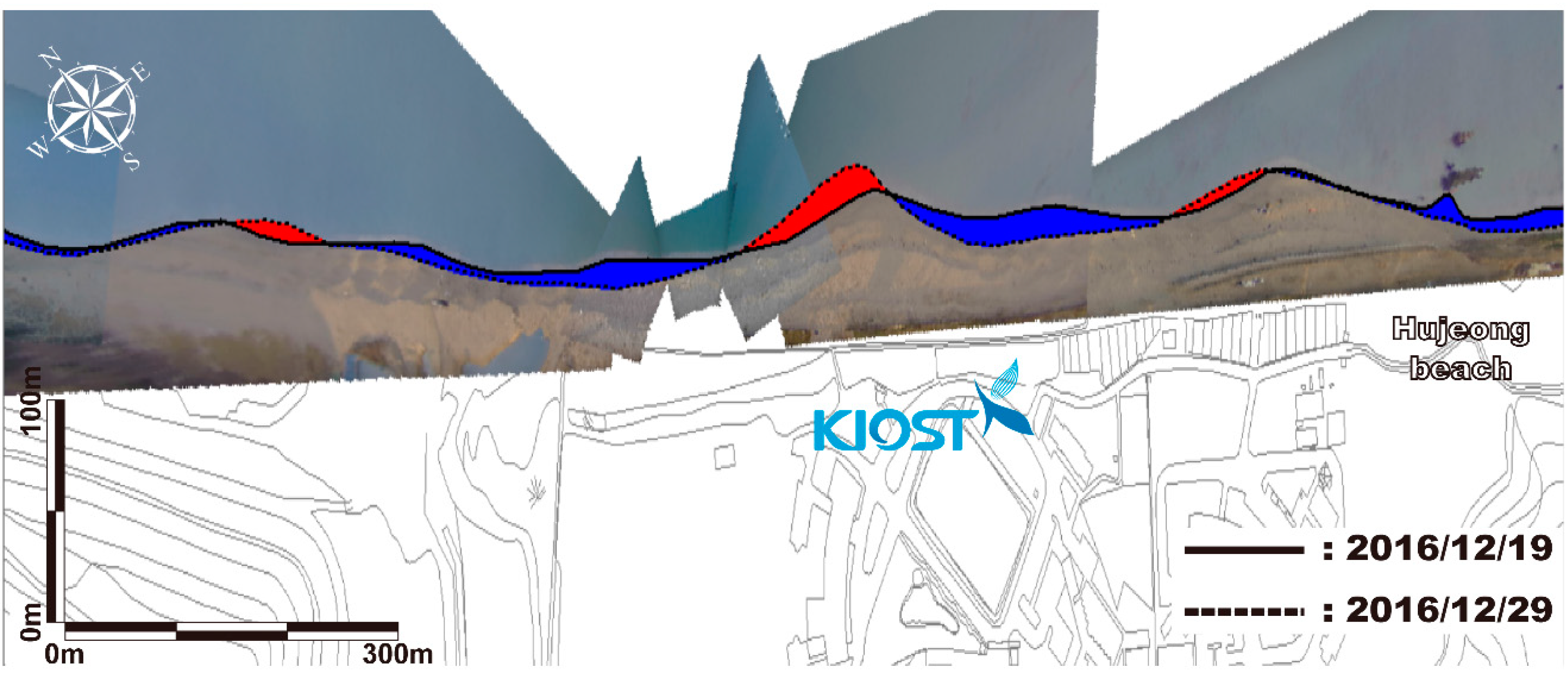
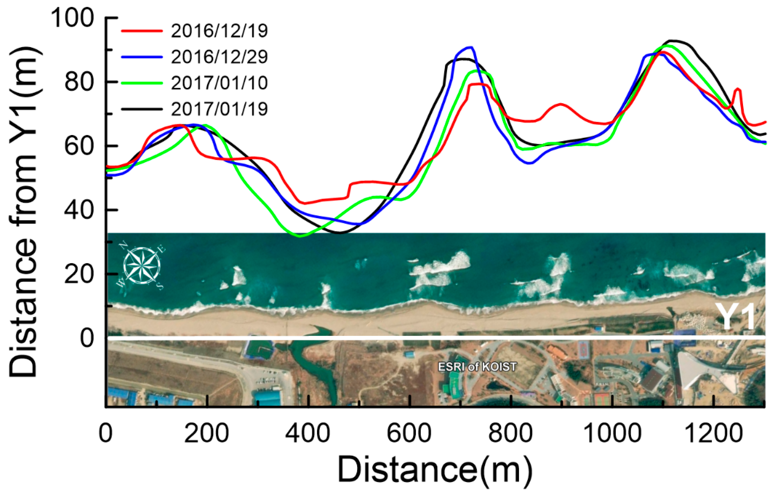
The shoreline changes measured by VMS are analyzed based on the hydrodynamic measurements. Figure 7 shows the shorelines measured on four different times around Exp#1, namely 19 December 2016; 29 December 2016; 10 January 2017; 19 January 2017. The shore was retreated between 19 December 2016 and 29 December 2016 in the majority of the sectors along the beach. This data can be compared with the hydrodynamic data in Figure 4 (t = – 1–9) in which two severe storms attacked the beach with strong nearshore currents and high wave nonlinearity, indicating that destructive forces might be dominant. However, there were locations where the shoreline was advanced. Specifically, the shoreline in the middle of the beach was significantly advanced during the storm. 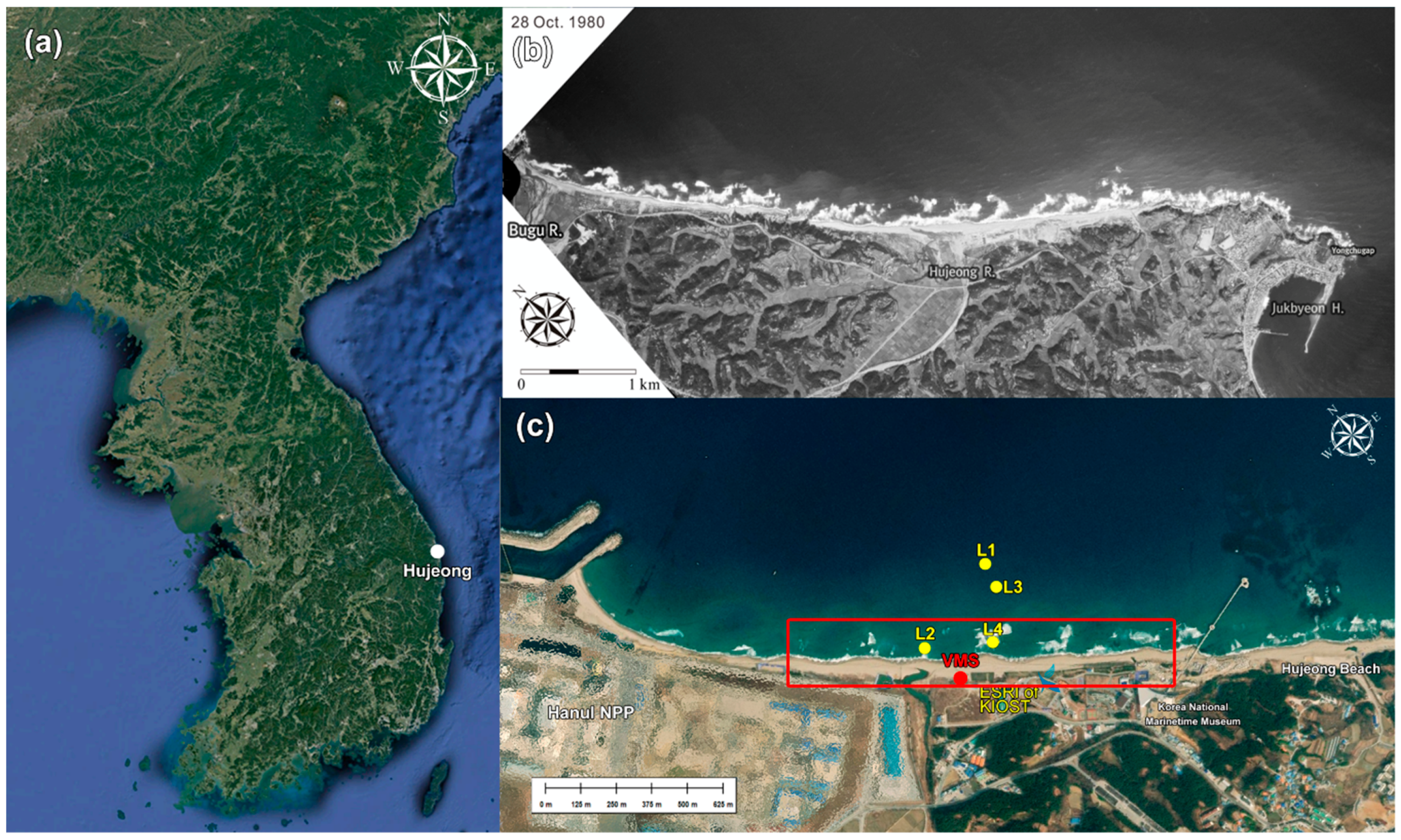Comparing the satellite image in Figure 3, this location corresponded to the protruded area connected to the horn of the crescentic sandbar. Therefore, the shoreline accretion can be interpreted as the wave energy was reduced over the shallow horn area due to enhanced wave breaking while the wave energy at other areas was relatively higher and the sediments were transported to be cumulated in the horn area.

Figure 7 also shows the shorelines measured by VMS at 29 December 2016 and 10 January 2017. This period corresponds to the time at t = 9–18 in Figure 4 when the wave energy became much lower without storm event. The shoreline change also shows no clear pattern of retreat or accretion. However, the northern part of the protruded area (left side in the figure) was eroded while the other side of it was advanced, which was likely related to the oblique wave incidence during t = 12–17 as shown in Figure 4b. The shorelines measured at January 10 and 19, 2017 shows the shoreline change pattern corresponding to the period of T2 of Exp#1. Interestingly, the shoreline was generally advanced in most of the sectors along the shore. The accretion of the shoreline in this period could not be understood considering the high wave conditions at t = 26–29 was considered (Figure 5). It may be related to the abnormally strong onshore currents observed in L2 at t = 26–29 (Figure 5b). However, the hydrodynamic condition in this period was similar to that observed at t = 3–6 when the storm waves attacked the shore, but the response of shoreline was opposite as it was advanced at t = 26–29 while it was retreated at t = 3–6, which may require further investigation.

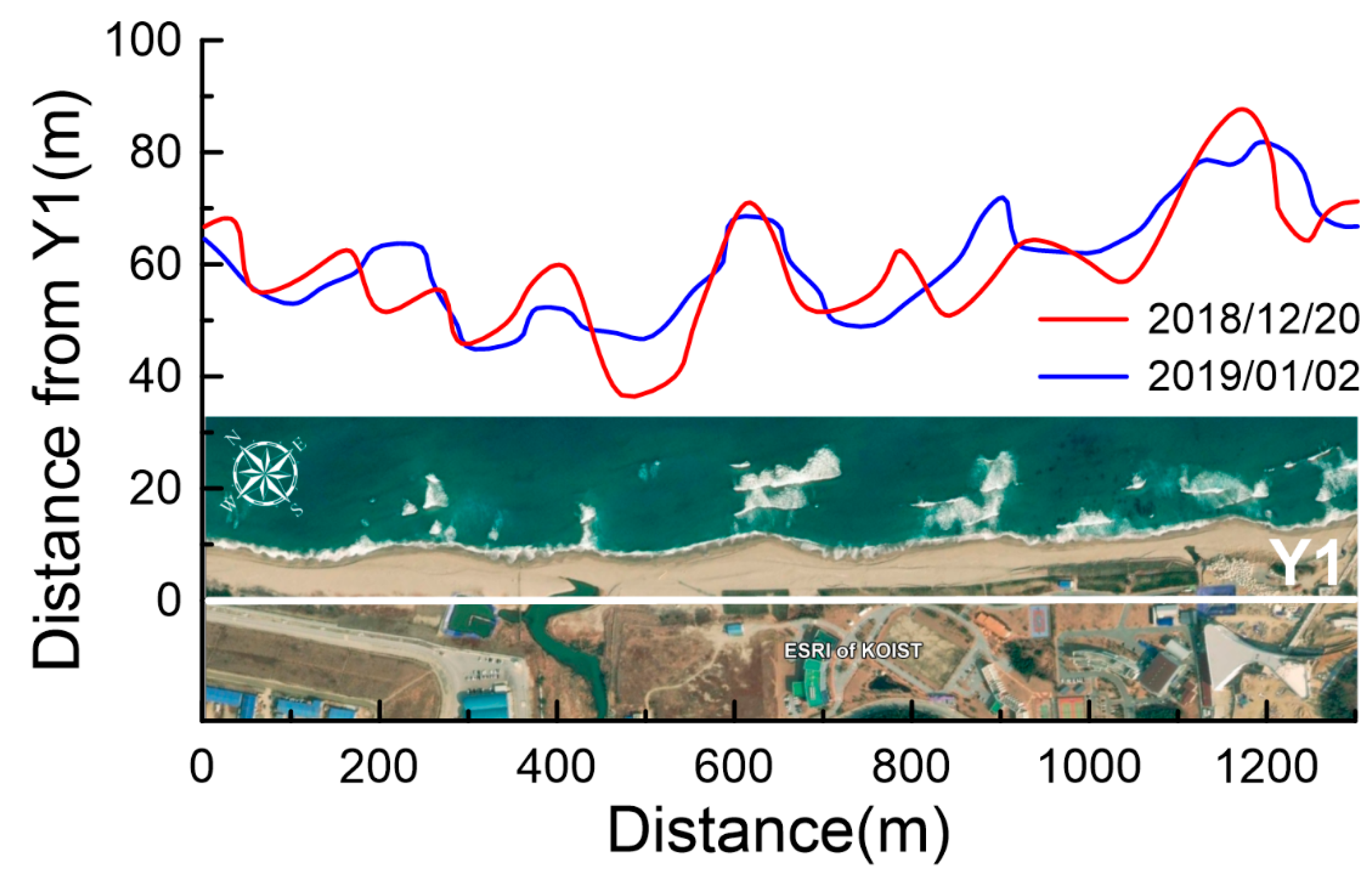
The shoreline change observed by VMS in Exp#2 is shown in Figure 8 where the shoreline positions are compared between 20 December 2018 and 02 January 2019 as it corresponds to the period in Figure 6. It should be noted that the shoreline feature was clearly different from those observed in Exp#1, which indicates that the shoreline had been actively changed during the ~1-year period between the two field experiments. It is also interesting to find out that the curved shoreline at 20 December 2018 became flattened at 2 January 2019 as the protruded areas were eroded while the caved areas were filled with the eroded sediments. Specifically, the eroded sediments moved south to fill the caved areas, which was likely due to the obliquity of the incident waves as it can be presumed from the wave direction in the corresponding period (Figure 6b).

3.3. Seabed Movement Detected by Satellite Images

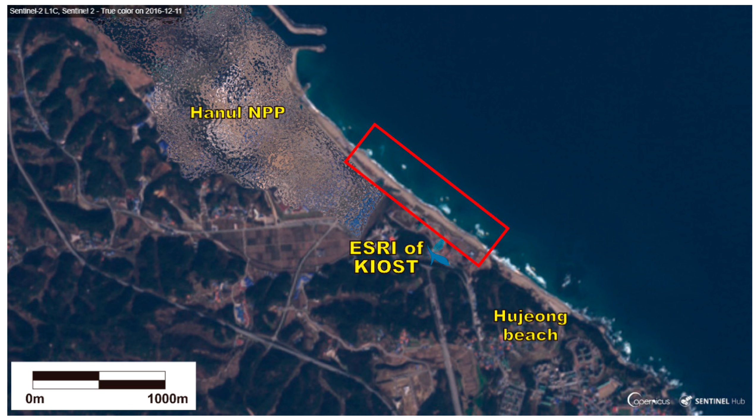
The Sentinel-II data in Figure 3 were plotted in RGB colors. In order to enhance the visibility of the underwater crescentic sandbars, the image was processed by applying the algorithm developed in [21] by which the position of nearshore sandbar crests was extracted from Sentinel-II images. In this study, the same algorithm was applied for the detection of sandbar positions. In this approach, calibrations based on in-situ measurements were not necessary to detect the positions of underwater sandbars. In addition, corrections of absolute values between different satellite images that might have different reflectance were not necessary either because the purpose was to extract the shape of response over underwater profiles perpendicular to the shoreline.

The readers are referred to [21] for the details of the sandbar extraction algorithm from Sentinel-II images, and it is only briefly summarized here. The first step was to extract the shoreline using a simple threshold applied to the short-wave infrared (SWIR) band because the spectral response of the water in the SWIR domain is almost equal to zero in low to moderate turbid waters from the resampling domain of 10 m spatial resolution. Then, a new raster, $r_a$, was defined by multiplying all visible bands in order to augment the increases in the spectral response over sandbars, such that $r_a=b_r*b_g*b_b$ where $b_r$, $b_g$, and $b_b$ represent the bands of red, green and blue respectively. Once $r_a$ distribution was calculated, a network of profiles perpendicular to the shoreline is created. The profiles started from the estimated shoreline, and the distance between two adjacent profiles was set to 10 m, which used total 210 profiles in this study. Along each profile, an exponential model, $\mathrm{y}=A*e^{\left(B*x\right)}+C$, was fit to the profile where coefficients $A$, $B,$ and $C$ were computed for each profile. After that, normalization of the profile was performed by subtracting the exponential model from the original profile. The shape of sandbar was then extracted along the profile using moving window.

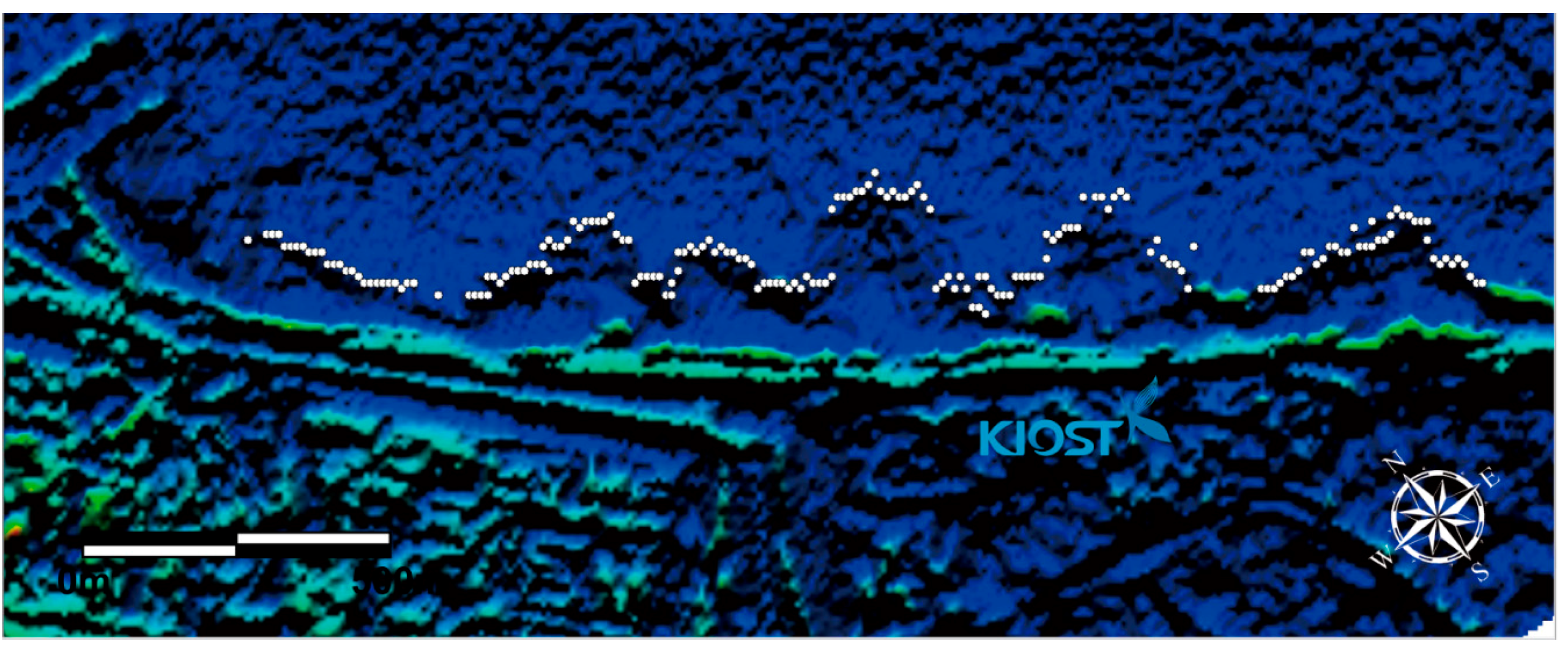
Figure 9 shows the converted Sentinel-II image of $r_a$ on 11 December 2016. In the water, the white dots denote the locations of the crest of sandbars as they were selected along each profile, and they generally correspond to the positions of sandbars expressed by the $r_a$ distribution. It shows that five crescentic sandbars of similar size were developed along the shore in the shallow nearshore area of the beach at depth of 3–5 m (the depths of bars were observed from the field measurements, not from satellite images). In the southeast part of the beach, sandbars could be hardly formed due to the existence underwater rocks. The horns of the bars (area where the bar is peaked toward the land) extended to the land as they were connected to the shore, on which the waves were breaking.

The image in Figure 9 was taken on 11 December 2016, nine days before the field experiment started on 20 December 2016. Although the Sentinel-II images are available for interval of 5–10 days, the sandbar data in Hujeong Beach were available on clear days only when the visible light could go through the water column to detect the seabed topography. For this reason, the next Sentinel-II image available in this site was measured on 31 December 2016, after the attacks of the two previous storms. The third Sentinel-II image available in the site was on 31 January 2017. Applying the same algorithm, the sandbar crest positions were extracted from the latter two images.

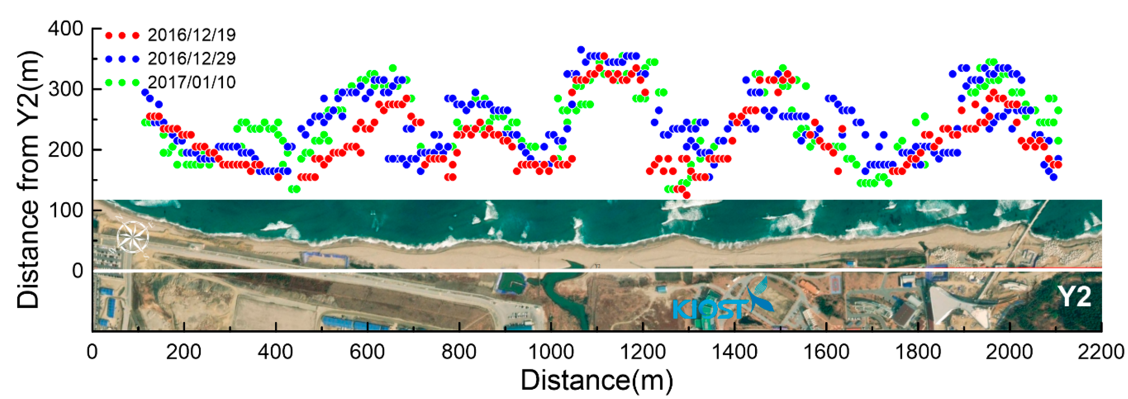
Figure 10 compares the locations of sandbar crest extracted following the algorithm by [21] between the three Sentinel-II images taken on 11 December (red dots), 31 December 2016 (blue dots), and 31 January 2017 (green dots). The bar crest locations of December 11 and 31 show that some parts of sandbars had moved offshore for maximum 70 m, which indicates the offshore sediment transport as it might be caused by the high storm waves that attacked the area on 23–25 December and 28–29 December 2016. The offshore movement of the sandbars corresponds to the results in the previous study [19] that reported a severe seabed erosion in L1 during the storm period on 23–25 December. It is also closely related to the hydrodynamic conditions in Figure 4 as it shows that the magnitude of wave skewness and asymmetry increased during the two storm periods. This indicates that the waves were likely breaking in L2 during the storms and the destructive forces such as undertow currents could become stronger to migrate the sandbars offshore. Once the wave condition became milder after the severe storms, the movement of the seabed contours was reduced. The sandbar crests measured on 30 January 2017 shows no clear difference with that on 31 December 2016, indicating that the seabed became stable without severe deformation though high wave conditions were observed during the period.

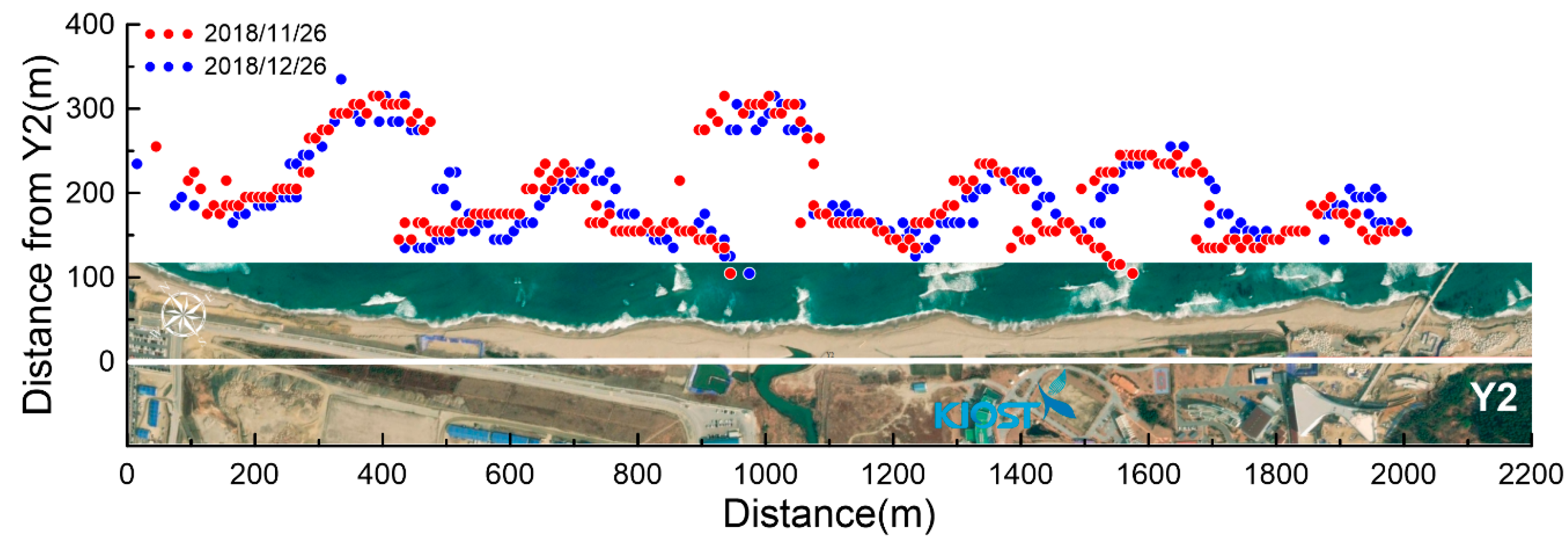
In Figure 11, the sandbar crest positions are compared between the Sentinel-II images taken on two days, 26 November 2018 (blue lines), 26 December 2018 (red lines) by applying the same algorithm. The two times were chosen at the dates when the Sentinel-II images were available around Exp#2. The figure shows that, though there was a one-month time gap between the two satellite images, the locations of seabed contours were similar indicating that the seabed morphology was stable during the period, regardless of the high wave conditions observed in Figure 6.

4. Discussion

One of the most significant findings in this study was that, under high wave conditions, the $S_k$ was reversed between the two stations located at different water depths. It was clearly observed during 24–26 December 2016 (t = 4–6 for Exp#1 in Figure 6) when the storm wave attacked the site with maximum $H_s$ of ~4 m. In this period, $S_k$ in L1 increased to become positive while it in L2 became negative. The positive/negative $S_k$ in L1/L2 was observed for longer period but with lower wave heights ($H_s$ = 2–3 m) during 15–19 January 2017 (t = 26–30 for Exp#1 in Figure 7). One possible explanation for this reversed sign in $S_k$ between the two depths can be found in the variation of wave nonlinearity of propagating waves. As the wave shoals in especially high wave energy conditions, $S_k$ would increase as the shape of surface waves become sharper. As the waves further propagate into the surf zone, the high storm waves would break and $S_k$ might change to be negative because the shape of surface waves is dispersed. The changes in $S_k$ along the wave propagation may also be closely related to the sediment motions in the seabed. When $S_k$ increased to become sharply positive in L1, the bed shear stress could be also increased to cause seabed erosion, which was observed in the previous study [18].

However, the seabed erosion implied from the high waves and the reversed $S_k$ measured at the two different water depths during the storm did not provide any clue to determine the direction of cross-shore sediment transport. As compared in Figure 6 and Figure 7, the hydrodynamic conditions during the two high wave conditions (t = 4–6 and t = 26–30 of Exp#1) were similar in the pattern of wave skewness as $S_k$ was positive in L1 but negative in L2. In addition, the cross-shore velocity in $\overline{u}$ showed that strong onshore currents were observed during both of the storm periods. However, the shoreline positions measured by VMS showed opposite pattern as it was generally retreated at t = 4–6 while it was advanced to the sea at t = 26–30. The reason for this discrepancy cannot be clearly understood based on the data available in this study. In fact, the seabed features detected by the satellite images confirmed the shoreline retreat at t = 4–6 because the crescentic sandbars moved offshore in the corresponding period. However, the shoreline accretion at t = 26–30 was not supported by the seabed data from satellite images, and thus the shoreline accretion at this time might not be directly contributed by the cross-shore sediment motions and further investigation may be required to analyze the direction of transport.

Although the wave skewness showed a pattern of significant changes in the waves that propagated into the surf zone under the two storm wave conditions, it was not observed at other high waves, which indicates that there might be other controlling factors that were not clarified in the present study. In addition, the wave asymmetry, another parameter for wave nonlinearity, did not show expected pattern by which, under storm wave conditions, $A_s$ would increase as the waves propagated into the surf zone. However, its magnitude was reduced close to zero under high wave conditions in both deep and shallow locations. Instead, $A_s$ was scattered with higher magnitude under mild wave conditions, especially when measured in shallower depths. The discrepancy in the wave nonlinearity between $A_s$ and $S_k$ could not be clearly understood in the present study, and it is suggested to inspect their relationship closely with additional data sets not only not only from this site but also from other sites with similar environment. However, there is a possibility that the high dispersion of $A_s$ could be contributed by the wider wave spectra in shallow water depths. When wave height became low under mild wave conditions, the wave measurement in shallow depths could be contaminated by the low flow velocities. As described in Table 1 and Table 2, the wave parameters were measured by ADCP and Signature in the deeper locations (L1 and L3) by shooting the soundwaves upward from the bottom, and the data were measured near the water surface. In the shallower locations (L2 and L4), the waves were measured by Acoustic Doppler Velocimeter (ADV) and the flow velocities were measured near the seabed so that their magnitude might be too small to accurately calculate the wave parameters. For example, the wave directions measured by same instruments show higher dispersion as well in the case of L2 and L4, which could be induced from the low flow velocities that might contaminate the accuracy of wave data.

Another discussion on the hydrodynamic measurement is the short period of data acquisition in Exp#2 due to burial of instruments at L4. It was unfortunate because the majority of data in Exp#2 could not be used in this study. Instead, it could be useful if the reason for the burial was analyzed based on the data available from the experiment. As shown in Figure 5, the instruments were buried in the beginning stage of storm wave period that had maximum wave height of ~2m, which was not extraordinary compared to the storm waves in Exp#1. However, one clue for the burial can be found from the shoreline changes measured by VMS in Figure 8 in which the shoreline positions compared for a period that contained the moment of instrument burial. As previously analyzed, the shoreline was flattened during the period mainly due to longshore sediment transport from NW, which was also confirmed from the hydrodynamic measurement in Figure 6c where strong longshore current was observed just before the time of burial. Therefore, it was likely that the instruments in L4 was buried by the sediments that were carried alongshore, not by the sediments carried from the shore.

One of the advantages of the present study is highlighted by the application of different sets of data available in the site. In addition to the hydrodynamic measurements at different water depths and at different times, the VMS data were useful to support the analysis. The hydrodynamic data alone could not understand the coastal process in general especially during the storm periods. The shoreline changes in the corresponding period could confirm the analysis of hydrodynamic data and thus prevent possible misinterpretation. Recently, the VMS techniques have been developed to various application in coastal areas. For example, it could be used to estimate breaking wave heights [28,29], to distinguish wave transformation domains [30], and to monitor shoreline response to nourishment [31]. These methods could be applied for the analysis of the VMS in the present experiment to extend the understanding of coastal processes in Hujeong Beach, and are thus suggested for future studies.

The satellite images were also effective to detect the significant changes of the bathymetry in shallow nearshore areas. Specifically, the Sentinel-II images applied in this study were useful for this type of analysis because of their relatively high spatial resolution and frequent orbital cycle. By applying the algorithm developed by [21] to extract the sandbar crest positions, it showed that the sandbars generally moved offshore for about 20–30 m with maximum 70 m during the period between December 11 and 31, 2016. This corresponds to the results by VMS data that shows the shoreline positions was also generally retreated for ~20 m during the corresponding period. The successful analysis of satellite data in the present study provides insights for the future application of the freely available remote sensing data for various purposes in coastal studies. The satellite images used in this study were taken in times when the wave condition was mild and the wave breaking heights were similar in all dates.

5. Conclusions

The hydrodynamics and wave nonlinearity of a field site were examined using the data sets measured at two different water depths and at two different times. Two experiments were performed to observe the changes of wave properties during the course of propagation into the surf zone, especially in storm periods, by mooring acoustic instrument for a couple of months. In addition to the hydrodynamic measurements, the video monitoring data that had recorded shoreline change information and satellite images were employed to support the analyses. The video monitoring data were measured by cameras on top of a 30-m high tower to extract the shoreline positions in the swash zone. The Sentinel-II satellite images, freely available, were useful to detect the changes in nearshore bathymetry on clear days because the satellite has high spatial resolution (~10 m) and frequent revisit cycle (~5 days).

The results showed that there were two storm periods (23–30 December 2016 and 15–19 January 2017) in which the maximum wave heights were higher than 2 m. The two cases had similar hydrodynamic conditions as strong onshore currents were observed at only shallower observational location during the storm periods. Specifically, in both storms, the wave skewness was reversed as the waves propagated because the skewness in deeper locations increased to become positive, but it decreased to become negative in the shallower locations, which indicates that the shoaling waves were broken as they propagated into the surf zone. In spite of the similarity in hydrodynamic conditions, the response of shoreline to these storm waves was different. In the period of the first storm, the shoreline was generally retreated. The erosional process was confirmed by the satellite data showing that the seabed was also moved offshore in the corresponding period. In the second storm period, however, the shoreline position was advanced to the sea. The similarity of hydrodynamic conditions but opposing pattern of shoreline responses in the two storms are not clearly understood based on the observational data available in the present study. One possible explanation can be found in the higher wave height in the first storm as its maximum wave height reached ~4 m, while it was less than 3 m for the second storm. In addition, the duration with high waves was longer for the first storm (~7 days), which likely enhanced the role destructive force supporting the erosion. Meanwhile, the wave skewness was significantly changed in time and space. The wave asymmetry, another parameter for wave nonlinearity, did not show any special pattern, even during the storm, which requires further investigation in future studies.