The Importance of the Coordinate Transformation Process in Using Heterogeneous Data in Coastal and Marine Geographic Information System

Abstract

Coastal and Marine Geographic Information Systems (CMGISs) permit to collect, manage, and analyze a great amount of heterogeneous data concerning coastal, sea, and ocean environments, e.g., nautical charts, topographic maps, remotely sensed images. To integrate those heterogeneous layers in CMGIS, particular attention is necessary to ensure the perfect geo-localization of data, which is a basic requirement for the correct spatial analysis. In fact, the above-mentioned types of information sources are usually available in different cartographic projections, geodetic datum, and scale of representation. Therefore, automatic conversions supplied by Geographic Information System (GIS) software for layer overlay do not produce results with adequate positional accuracy. This paper aims to describe methodological aspects concerning different data integration in CMGIS in order to enhance its capability to handle topics of coastal and marine applications. Experiments are carried out to build a CMGIS of the Campania Region (Italy) harmonizing different data (maps and satellite images), which are heterogeneous for datum (World Geodetic System 1984 and European Datum 1950), projection (Mercator and Universal Transverse of Mercator), and scale of representation (large and medium scale). Results demonstrate that automatic conversion carried out by GIS software are insufficient to ensure levels of positional accuracy adequate for large scale representation. Therefore, additional operations such as those proposed in this work are necessary.

1. Introduction

A Geographic Information System (GIS) is a computer system that allows the capture, storage, query, analysis, and display of geospatial data [1]. It provides functionality for computerized mapping and spatial analysis that permits a better understanding and modelling of real-world phenomena [2]. By the use of spatial location, GIS integrates many different kinds of data layers including imagery, features, and base maps [3].

In recent years, GISs have increased their presence as tools to better understand and manage coastal and marine environments [4]. As a consequence, the term “Coastal and Marine Geographic Information System” (CMGIS) has been introduced to indicate the GIS application was finalized to integrate heterogeneous data concerning coastal, sea, and ocean environments. The applications cover several aspects, e.g., ecological studies [5], water quality [6,7], coastal erosion [8,9], aquaculture [10], oil pipeline route optimization [11], etc. The primary source of information for many applications are nautical charts [12] that provide the shape and position of the shoreline, conformation of the seafloor, water depths, locations of dangers for navigation, positions and characteristics of aids to navigation, anchorages, and other features. Nautical charts in digital form are the base for an Electronical Chart Display Information System (ECDIS) that is a GIS system designed for marine navigation, according to the relevant standards of IMO (International Maritime Organization) [13]. Furthermore, it is one of the most useful equipment on the bridge because of its ability to warn the user of approaching shallow water [14]. The nautical chart information is useful not only for navigation, but also for other applications concerning, for example, marine and ocean currents, environmental changes, fishing resources, etc. However, a better description of sea bottom morphology can be achieved by the hydrographic survey [15]. GIS interpolation tools permit us to process single beam data for 3D models [16,17] that integrate nautical chart information. In order to provide detailed information about coastal zones, nautical charts are limited. Therefore, topographic maps [18] are necessary to show both natural and man-made features at a large scale of representation. Remotely-sensed images can supply other precious information for CMGIS [19] covering many aspects of the sea and ocean waters (e.g., temperature, pollutions, ice) as well as land configuration and use.

When using such heterogeneous layers, the problem is to ensure the perfect geo-localization of data [20]. In many cases, automatic conversions supplied by GIS software for layer overlay do not produce results with adequate positional accuracy because of different geodetic datum, cartographic projections, and scale of representation. A geodetic datum is a tool used to define the shape and size of the earth as well as a set of reference points used for locating places on the Earth. Throughout time, hundreds of different datums have been used with each one changing with the historical period and/or the geographic area [21]. A cartographic projection is a way to flatten the earth model’s surface into a plane in order to produce a map by transforming latitudes and longitudes of localities from the globe into locations on a plane [22]. The number of possible map projections is unlimited [23]. However, apart from the literal significance, projection is not limited to map points in three-dimensions onto a two-dimensional plane using geometrical construction based on the use of lines of sight from the object to the projection plane. In fact, any mathematical function transforming spherical or ellipsoidal coordinates from the earth model’s surface to the plane is a projection [24,25]. The map projections that are of a real perspective are few. The scale of a map, resulting from the ratio of a distance on the map to the corresponding distance on the ground [26], assumes different values for CMGIS usually ranging from 1:10,000,000 or minus (geographic maps) to 1:500 (technical maps).

It is strictly necessary to know the accuracy of the input data in order to be able to evaluate the reliability of the processed data. Furthermore, GIS data processing generates the persistence of an error into new datasets calculated or created using datasets that originally contained errors. The study of error propagation is extremely important because it permits us to estimate the effects of combined and accumulated errors throughout a series of data processing operations [27]. Errors can be injected at many points in a GIS analysis, and one of the largest sources of error is the data collected. Each time a new dataset is used in a GIS analysis, new error possibilities are also introduced because GIS permits us to use information from many sources. It is necessary to have an understanding of the quality of the data [28]. For consequence, spatial metadata, used to provide information about the identification, the extent, the quality, the spatial and temporal aspects, the content, the spatial reference, the portrayal, distribution, and other properties of digital geographic data and services [29,30], is a fundamental part of any spatial data set, which enables us to organize, share, and use spatial data [31].

Any measurement-based spatial data sets are susceptible to uncertainty. If this uncertainty was not taken into account, the search would produce inaccurate results. If the information system in which one operates ignores the uncertainty of the data, it is up to the operator to take it into consideration [32]. Many studies are available in literature on the impact of quality data on GIS uncertainty. In relation to weather-related disasters, researchers in Reference [33] focused their study on assessing the state of spatial information quality for hydrodynamic modeling needs. Particularly, they carried out an assessment of the qualitative analysis on three levels, i.e., main channel and surrounding topography data from geodetic measurements, digital relief model, and hydrodynamic/hydraulic modeling, and demonstrated that the qualitative aspect of the input data shows the sensitivity of a given model to changes in the input data quality condition.

Even if the quality of the input data is high, the overlapping and interaction operations between layers, in the absence of particular attention to the procedures performed, can give rise to high levels of uncertainty. Sources of error become the transformations of cartographic projection, coordinate type, and datum. The error propagation typical of GIS can take on even more serious connotations in the case of CMGIS due to their very nature and characterization. The CMGIS deal with both land and sea at the same time. Two areas are usually characterized by different cartographic projections [34]. In addition, the need to compare time sequences of data makes it mandatory to use recent and non-recent data with different datum and type of coordinates, e.g., for coastline [35,36] and bathymetry change analysis [37].

The main goal of this paper is to demonstrate that the results achievable with automatic coordinate transformation carried out by GIS tools can be incompatible with the reference scale of the source data. In other words, they significantly worsen the accuracy of the results and do not ensure levels of positional accuracy adequate to large scale representation. For consequence, additional operations as those proposed in this work are necessary. The novelty of this article is to define technical solutions in order to achieve accurate overlap between heterogeneous layers in CMGIS, which is a fundamental requirement for conducting reliable spatial analysis on them. Spatial analysis is a type of geographical analysis that seeks to explain patterns of human behavior as well as natural phenomena and their spatial expression in terms of mathematics and geometry [38]. It represents the very crux of GIS, which adds value to geographic data that converts data into useful information and knowledge [39]. When the characteristics of the study area are reported in different layers, the perfect overlay of them is fundamental to detect a link between the phenomena in order to obtain high quality results.

The article is organized as follows. Section 2 describes the experimental framework used to evaluate the performance of the proposed approaches for CMGIS by outlining the main characteristics of the geographical area considered, the Campania coasts, and the stretch of sea in front of them. Section 3 introduces data used throughout this paper. Six different datasets are considered in order to analyze some recurrent problems of the coordinate, projection, and datum transformations. Section 4 reviews the traditional methods for georeferencing, ortho-rectifying, re-projecting, and datum transforming, and gives the details of their implementation and optimization. Section 5 outlines and discusses the results of this study. Section 6 presents our conclusions.

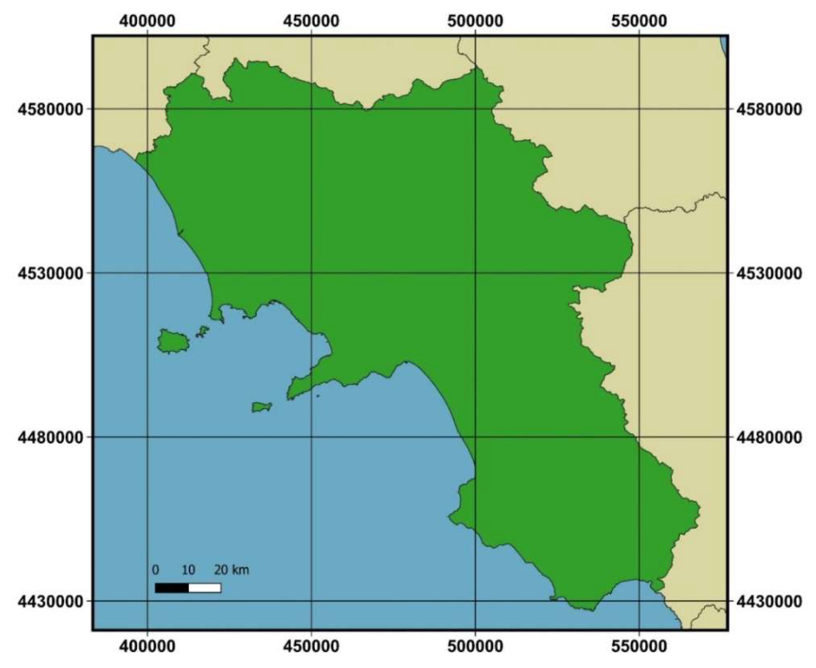
2. Study Area

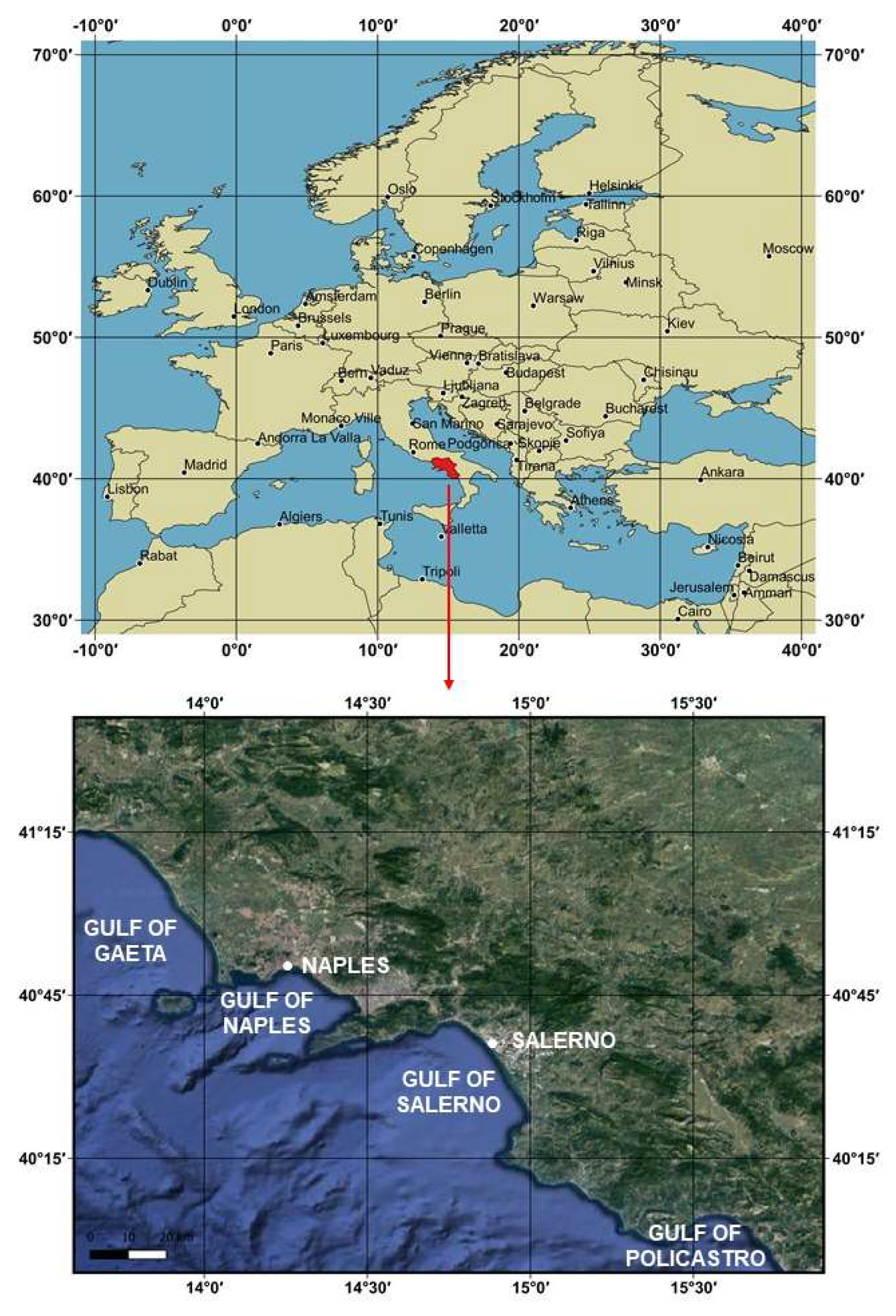
The study area chosen for this work concerns the Campania region (Figure 1).

This region, located in the south of Italy, is characterized by a coast that extends mainly in the north-west, south-east direction. The coastline has a length of about 450 km [40]. Four main Gulfs (Gaeta, Naples, Salerno, and Policastro) and three isles (Capri, Ischia, and Procida) can be identified. The central coast of the region is mostly high and rocky with volcanic ridges. The Gulf of Gaeta, located between the Lazio Region and Campania Region, presents the coast as characterized by flat and accessible beaches, covering many kilometers before getting steeper (the coasts of the Gulf of Gaeta are low and bordered by dunes). The Gulf of Naples has many bays and coves. The Gulf of Salerno is separated from the Gulf of Naples (on the north) by the Sorrentine Peninsula, while, from the south, it is bounded by the Cilento coast. The northern part of this coast is the touristic Costiera Amalfitana, including towns like Amalfi, Maiori, Positano, and the city of Salerno itself. The coasts of the Gulf of Salerno are flat in correspondence of the river Sele, but higher elsewhere and rich in small coves. The Cilento peninsula, which is south of the Gulf of Salerno, has rather inhospitable coasts with shaken banks.

The study area is particularly interesting in many respects. The geophysical [41], climatological [42], and ecological [43] characterizations of this area justify the need to create a CMGIS. Coastal hazards are identified in this region, especially in northern Campania, which was defined during an International Workshop on the Integrated Coastal Zone Management in 1999 as “a broad urbanized coastal zone with a variety of conflicting land uses” [44]. Northern Campania also presents very intense phenomena of coastal erosion and many studies starting from 1980 have analyzed the coastline variation in this area [45,46] by identifying the alteration of the sedimentary cycles and the littoral dynamics as well as the modification of the coastal dunes as the main causes of the morphological variation [47]. Particularly interesting for continuous changes is the coastal evolution in the Volturno delta system and domitian area. In References [36,48,49], researchers used wide databases comprising historical maps, aerial photographs, topographic sheets, bathymetric data, and satellite images to extract the spatial and temporal information of the coastlines at several time points, and the comparison of different layers required accurate overlapping [36,48,49].

The use of heterogeneous data characterizes study and research activities focused on the coastal erosion as well as other phenomena that can be investigated using spatial analysis tools. The search for solutions capable of achieving the perfect overlapping of the layers certainly constitutes a necessary exercise that systematically involves the scholar who is preparing to create a CMGIS. The proposed area, due to the presence of phenomena of geophysical, environmental, and ecological interest, as well as the wide availability of data, is particularly emblematic of some recurrent problems that require accurate solutions.

3. Data

To treat the problem of harmonizing heterogeneous data, the following data sources are considered.

• Topographic Map of Naples n° 447-II, produced in 1997 by Istituto Geografico Militare Italiano (IGMI), in scale 1:25.000, referred to European Datum (ED50),
• Nautical Chart n° 130, produced in 1996 by Istituto Idrografico della Marina Militare (IIMM), on the scale 1:30.000, referred to ED50,
• GeoEye-1 satellite imagery, acquired on 07/04/2012, resolution 2 m for multispectral bands, 0.5 m for panchromatic band, referred to as World Geodetic Datum (WGS84),
• Vector layer of administrative bounders of Italian Regions, updated in 2020, n scale 1:50,000, referred to as WGS84,
• Electronic Navigational Chart (ENC) n° 84 of the Port of Naples, produced in 2019 by IIMM, on the scale 1:10.000, referred to WGS84.

The point cloud dataset concerning single beam echo-sounder bathymetric survey of the Baia of Pozzuoli carried out in 1970 by IIMM on a scale of 1:10.000, which is referred to as ED50.

The different production dates reflect the particularity of the CMGIS that are often applied to themes and geographical areas that require the use of layers dating back to different time locations.

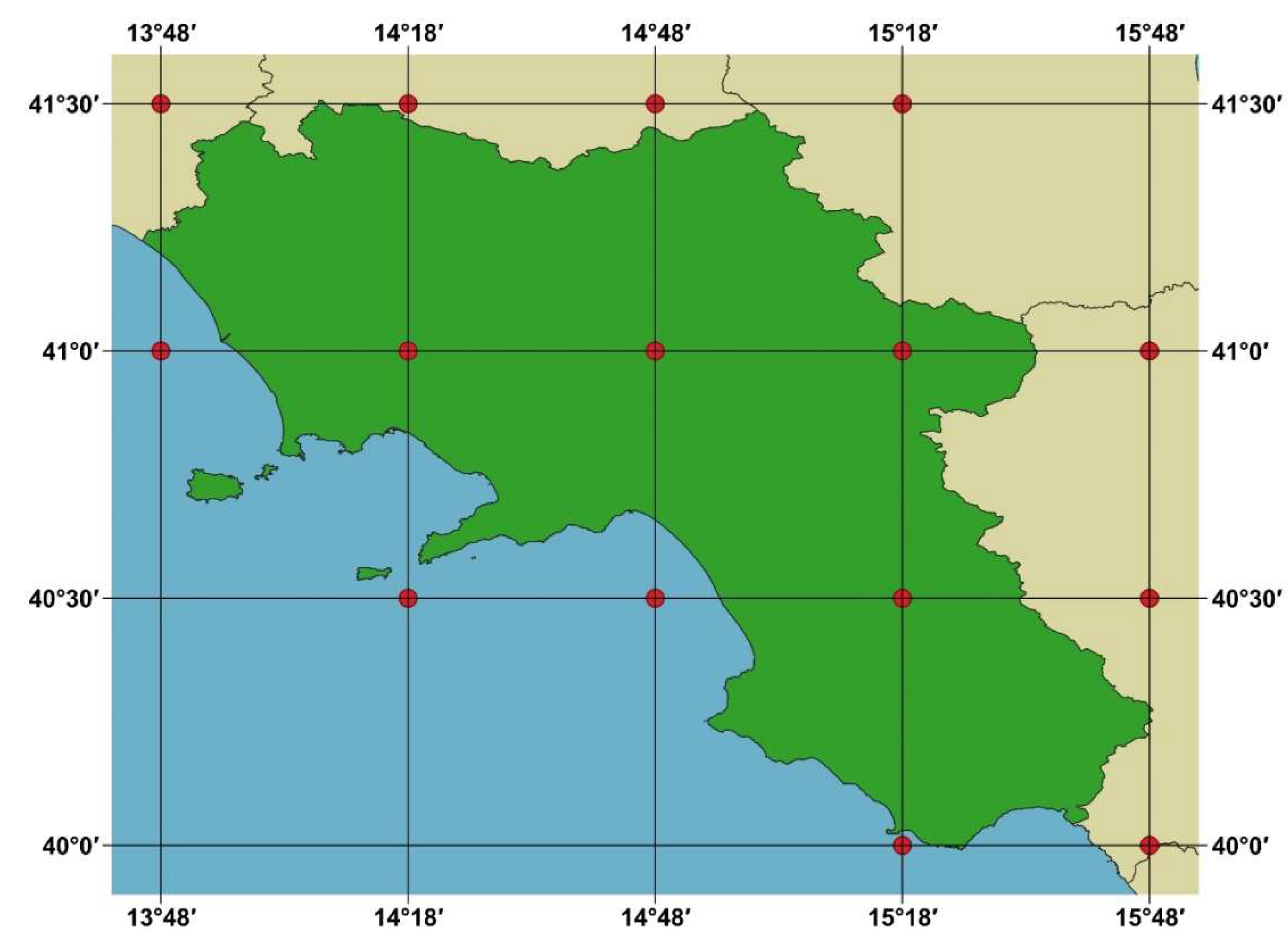
The geolocations of the data sources are shown in Figure 2.

The Dataset (1) results from the scan of a topographic map in a paper form produced by the Italian Mapping Agency (Istituto Geografico Militare Italiano, IGMI). The map projection is the Universal Transverse of Mercator (UTM) characterized by a function, F, which takes a latitude and longitude, along with specific parameters, and returns the northing and easting. F is specified as:

F: (ϕ, λ, ϕ₀, λ₀, k₀, a, e², FE, FN) → (N, E)

(1)

The parameters for F are:

• ϕ = the latitude
• λ = the longitude
• ϕ₀ = the projection center latitude
• λ₀ = the projection center longitude
• k₀ = the scale factor of the projection
• a = the semi-major axis of the ellipsoid
• e² = the square of the eccentricity of the ellipsoid
• FE = the false easting of the projection
• FN = the false northing of the projection
• N = the northing
• E = the easting

To compute easting and northing values, the function F makes use of two equations that can be easily found in literature [50,51,52].

The UTM system divides the Earth into 60 zones, each 6° of longitude in width. Zone 1 covers longitude 180° W to 174° W. Zone numbering increases eastward to zone 60, which covers longitude 174° E to 180° E. The polar regions south of 80° S and north of 84° N are excluded. In each zone, the scale factor varies from 0.9996 to 1.0004. FN is 10.000 km in the Southern hemisphere, 0 km in the Northern one. FE is 500 km in both hemispheres. UTM can be applied to a specific geodetic datum.

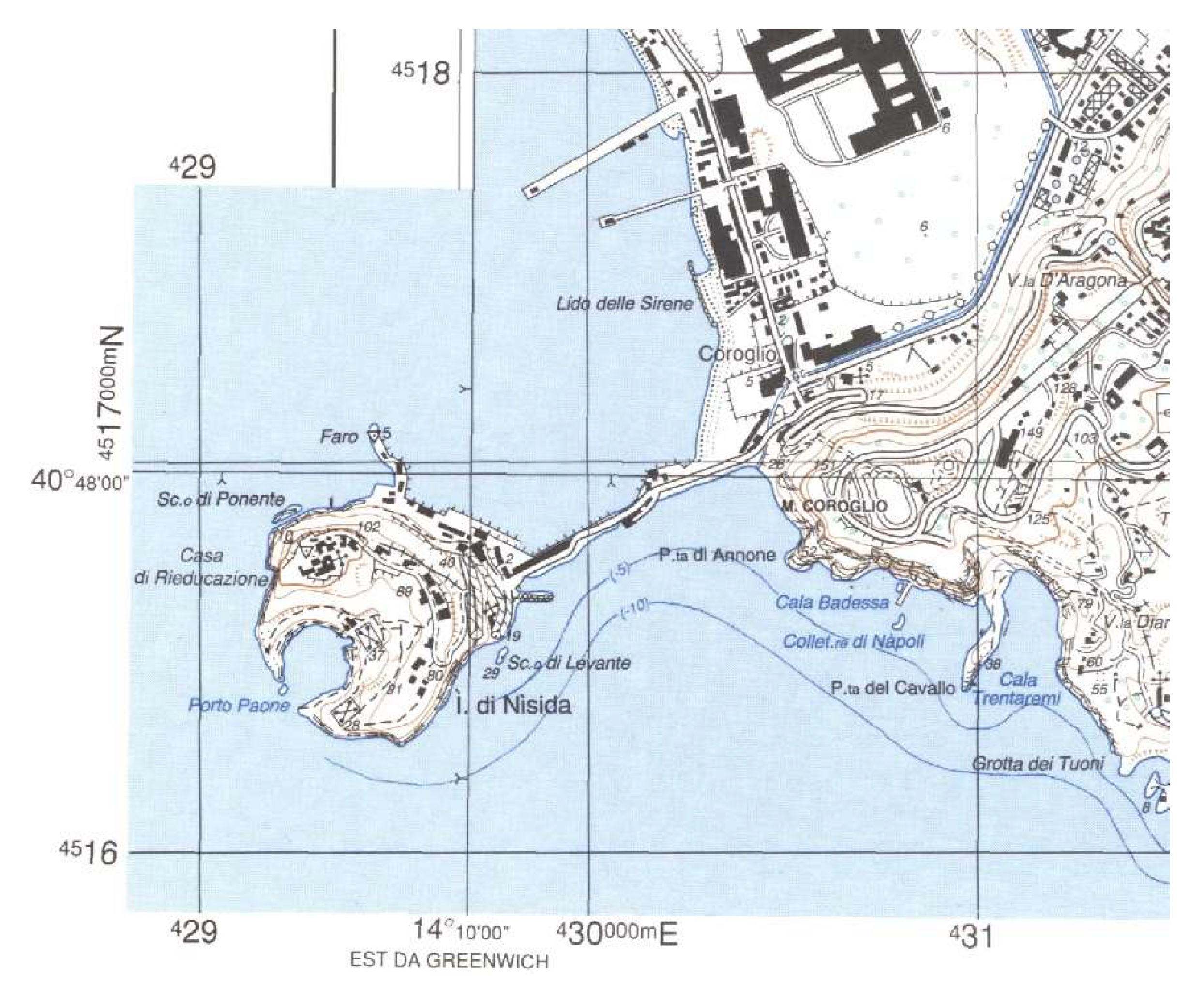
In this case, the map is referred to as the European Datum (ED50) and corresponds to the zone 33 N. It covers an area of about 193.639525 km², including the Municipality of Naples, within the following UTM/ED50 zone 33 N plane coordinates: E₁ = 428,840 m, E₂ = 443,845 m, N₁ = 4,515,165 m, and N₂ = 4,528,070 m. A detail of this map concerning the isle of Nisida (between Naples and Pozzuoli) is reported in Figure 3.

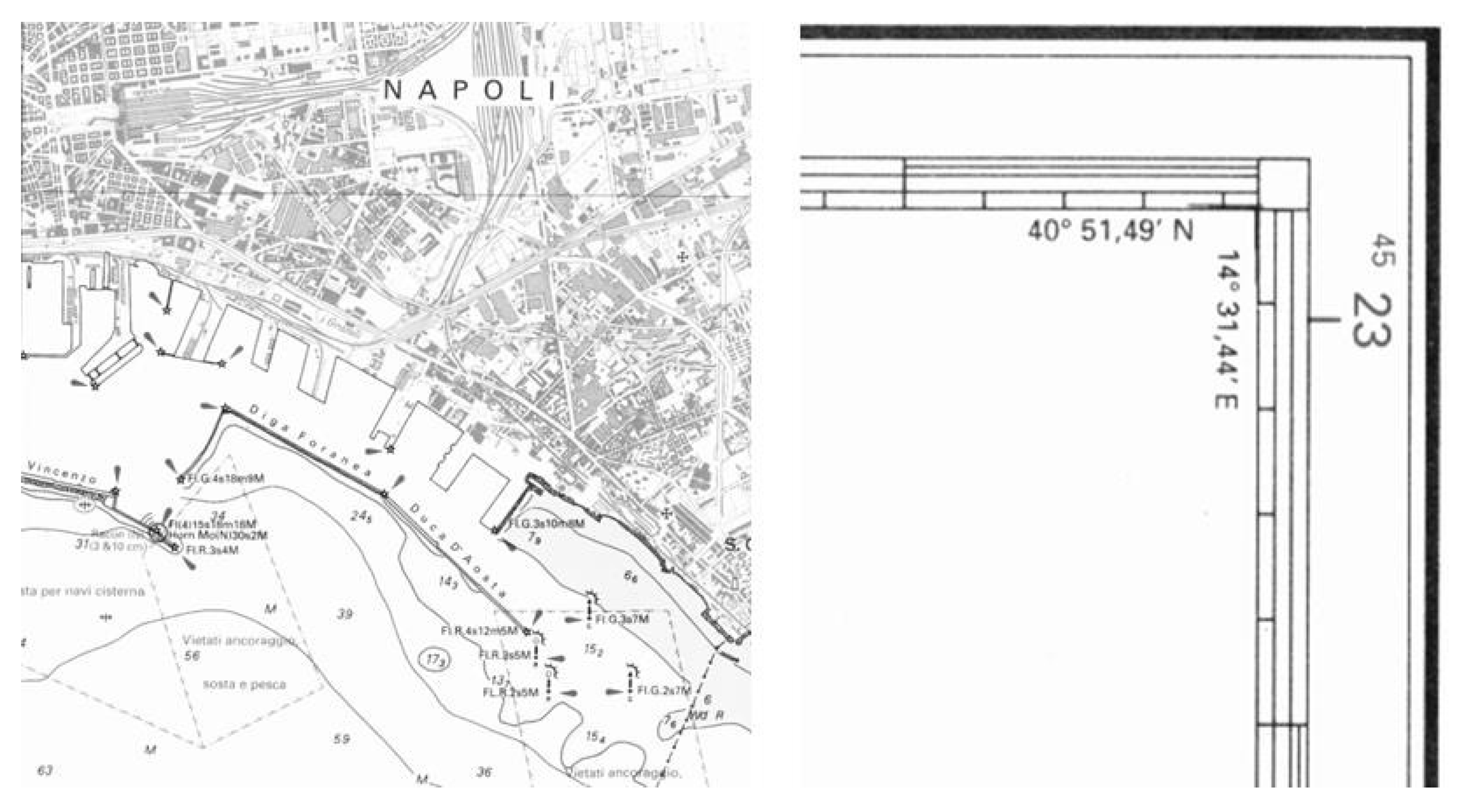
The Dataset (2) results from the scan of a nautical chart in paper form produced by the Italian Hydrographic Office (Istituto Idrografico della Marina Militare, IIMM) in scale 1:30.000. It covers a large area of the gulf of Naples with its extension comprised between 14°08.00′ E and 14°31.44′ E of longitude and 40°39.33′ N and 40°51.49′ N of latitude (including an area of about 746.26 km²). Referred to as ED50, it is designed in Mercator cartographic representation using the parallel at 40° 45′ N as a standard to reduce deformations in the represented area. The map equations are:

$$\begin{array}{c}\mathrm{x}=\mathrm{a}\left({\lambda -\lambda }_0\right)·\frac{{\cos \mathsf{\phi }}_1}{\left(1-{\mathrm{e}}^2{\sin }^2{\mathsf{\phi }}_1\right)}\\ \mathrm{y}=\mathrm{aln}\left[\tan (\frac{\mathsf{\pi }}{4}+\frac{\mathsf{\phi }}{2})·{\left(\frac{1-\mathrm{esin}\mathsf{\phi }}{1+\mathrm{esin}\mathsf{\phi }}\right)}^{\frac{\mathrm{e}}{2}}\right]\frac{{\cos \mathsf{\phi }}_1}{\sqrt{\left(1-{\mathrm{e}}^2{\sin }^2{\mathsf{\phi }}_1\right)}}\end{array}$$

(2)

where:

• ln is the neperian logarithm,
• a is the equatorial radius,
• e is the eccentricity of the ellipsoid,
• $\mathsf{\lambda }$₀ is the longitude of the y—Axis,
• $\mathsf{\phi }$₁ is the latitude of the standard parallel.

The map is reported in Figure 4.

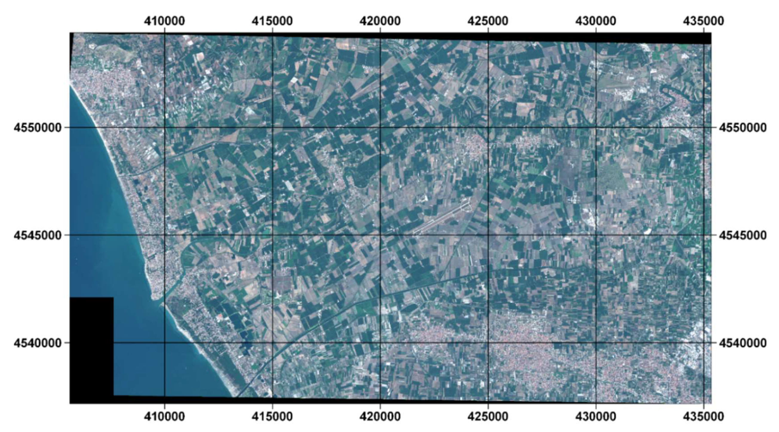
The Dataset (3) is a GeoEye-1 imagery, acquired on 07/04/2012, including one panchromatic image (Pan: 0.450 μm–0.800 μm) with a cell size of 0.50 m × 0.50 m and four multispectral images (Blue: 0.450 μm–0.510 μm; Green: 0.510 μm–0.580 μm; Red: 0.655 μm–0.690 μm; Near-Infrared: 0.780 μm–0.920 μm) with pixel dimensions of 2.0 m × 2.0 m [53]. GeoEye-1 imagery as well as Very High Resolution (VHR) images are useful for many GIS applications, e.g., identification of flooded areas [54], Digital Terrain Model (DTM) production [55], forest monitoring [56], etc. However, those images have gradually spread more in the CMGIS applications because of the presence of multispectral data that, opportunely processed, provide information about many aspects, such as sea-bottom morphology [57] and types [58], coastline shape, and position [59]. The dataset supplied by the provider as standard geometrically correct, geo-referred to as WGS84 and in UTM projection, covers an area of about 514.22 km², located around Volturno river, from Capua to the Tyrrhenian sea. Particularly, it extends within the following UTM/WGS84 plane coordinates—33T zone: E₁ = 405,540, E₂ = 435,350 m, N₁ = 4,537,164 m, N₂ = 4,554,414 m. The Red-Green-Blue (RGB) true color composition obtained with bands 3, 2, 1 concerning the whole considered scene is reported in Figure 5.

The Dataset (4) is a clipped vector layer of Italian Region administrative boundaries reporting Campania and neighboring areas. The dataset is geo-referred in UTM/WGS84 Zone 33 N and covers an area of about 35,891.44 km², within the following plane coordinates: E₁ = 383,331 m, E₂ = 576,936m, N₁ = 4,417,046 m, N₂ = 4,602,291 m. The clipped vector layer is reported in Figure 6.

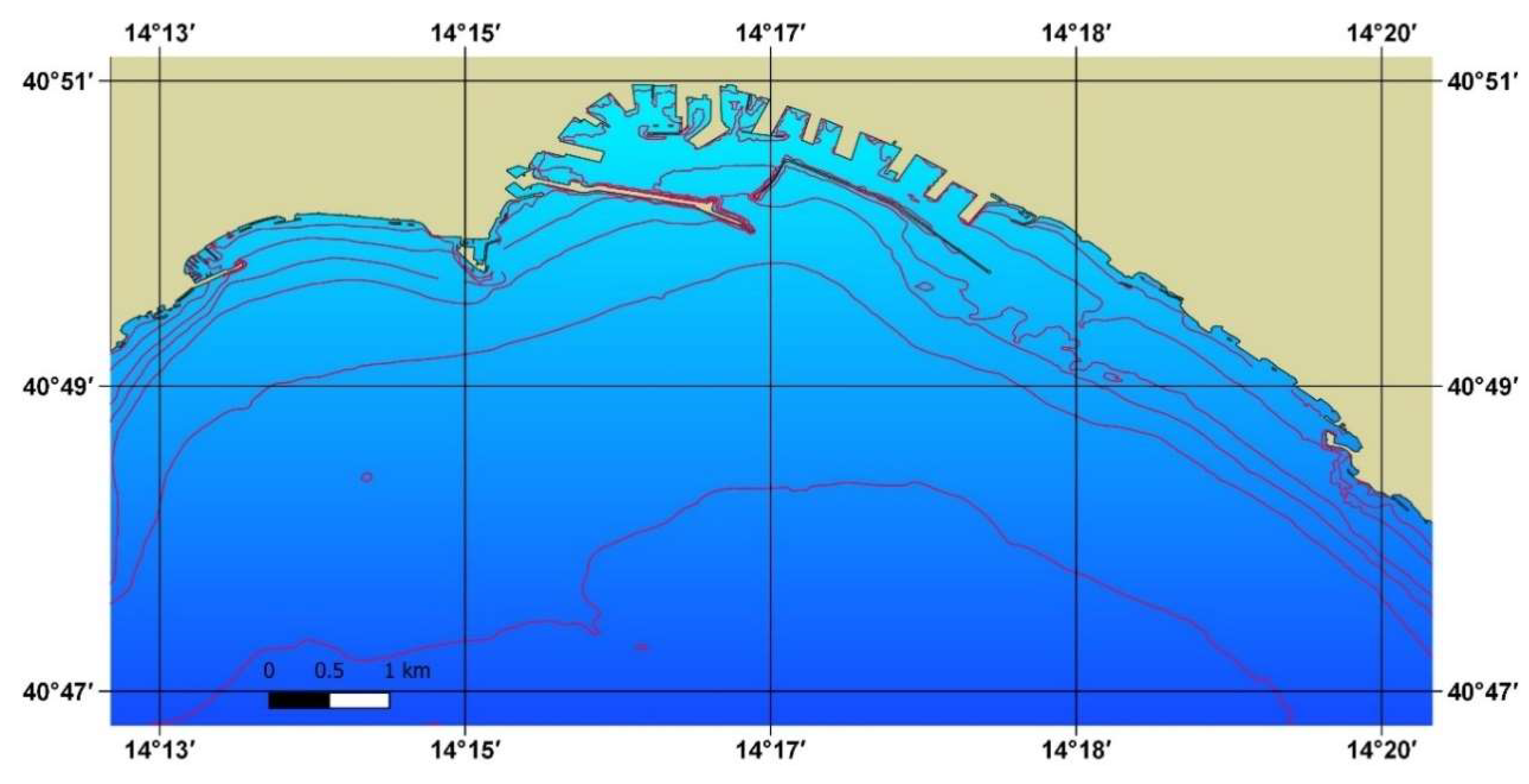
The Dataset (5) is the ENC of the Port of Naples, produced in 2019 by IIMM, on a scale of 1:10.000. This layer is formed in accordance to the official standards established by the International Hydrographic Organization (IHO). Particularly, it is conformed to S-57 IHO Transfer Standard for Digital Hydrographic Data, which is the primary standard used for ENC production that includes a description of objects, attributes, data encoding format, and a product specification and updating profile [60]. ENC is geo-referred to WGS84. The projection is not defined and the system that read the information visualizes it in the system default projection, i.e., equi-rectangular projection for QGIS. The equirectangular projection is also called the equidistant cylindrical projection or geographic projection. It plots meridians to vertical straight lines of constant spacing and parallels to horizontal straight lines of the constant. The projection is neither conformal nor of an equal area [23]. The layer visualization in QGIS (limited to depth contours and coastline) is reported in Figure 7.

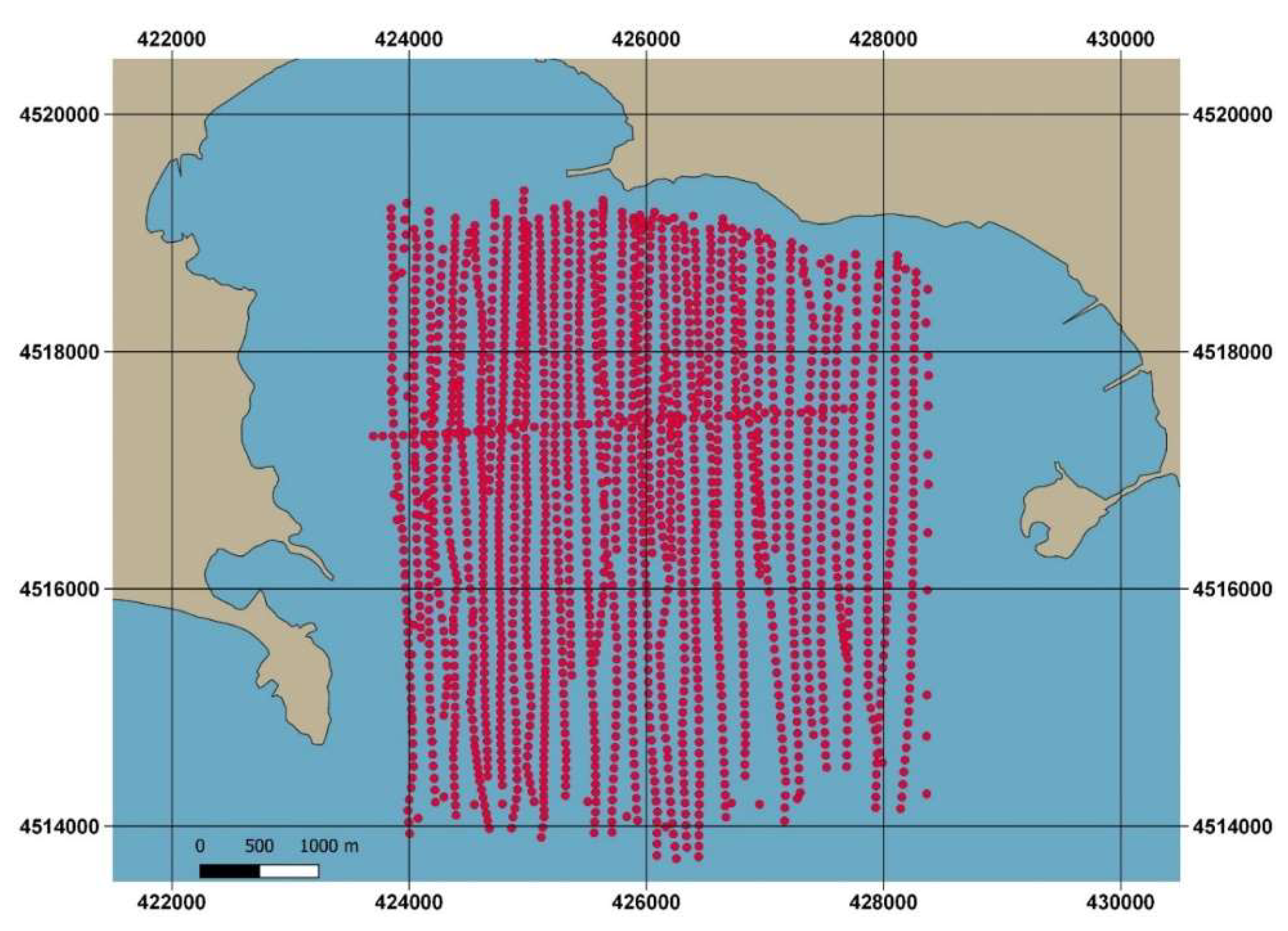
The Dataset (6) is a point cloud dataset concerning seabed morphology of the Baia of Pozzuoli. Acquired in 1970 by IIMM, using a single-beam echo-sounder, the dataset is a 3D shapefile in scale 1:10.000, geo-referred to UTM/ED50 and corresponds to the zone 33 N. It covers an area of about 26.3675 km², within the following UTM/ED50 zone 33 N plane coordinates: E₁ = 423,697.89 m, E₂ = 428,377.39 m, N₁ = 4,513,725.80 m. N₂ = 4,519,357.15 m. The layer visualization in QGIS (2D representation) is reported in Figure 8.

4. Methods

4.1. Georeferencing

The raster and vector files relative to the digitizing of a map gain real cartographic meaning only through the process of georeferencing [61]. Georeferencing requires the use of software that can assign new coordinates to the starting file by applying a geometric transformation. The user must indicate the initial and final coordinates for some points. The software automatically determines the final coordinates of all points and places the image (or vector layer) in the new position [62].

To place the raster image or the vector layer in the chosen cartographic space, a geometric transformation is carried out. In the simplest case, it is limited to a roto-translation with variation of the scale factor (conformal transformation) [63].

Said x, y are the coordinates of a generic point P of the starting layer and said x’, y’ are the corresponding coordinates of the same point in the cartographic representation of arrival. The conformal transformation has equations:

$$\begin{gathered} x^{\prime }=ax+by+c \\ {y}^{\prime }=-bx+ay+d \end{gathered}$$

(3)

Once the four parameters a, b, c, and d have been determined, it becomes possible to calculate x’, y’ as a starting point from x, y. To achieve this goal, it is necessary to know the x, y coordinates of at least two known points in the starting layer and the x’, y’ coordinates of the corresponding points in the final one in order to solve the system of four equations in four unknowns whose solutions provide the unknown parameters [64].

The conformal transformation is a particularization of the affine transformation that is characterized by the equations:

$$\begin{gathered} x^{\prime }=ax+by+c \\ {y}^{\prime }=dx+ey+f \end{gathered}$$

(4)

The affine transformation permits a rotation, a translation in x and y, scaling along both axes, and an obliquitous transformation. To determine the parameters a, b, c, d, e, and f, it is necessary to know the x, y coordinates of at least three points in the starting layer and the coordinates x’, y’ of the corresponding points in the final one [65].

The affine transformation is included into the category of the two-dimensional (2D) polynomial functions (PFs) used for image georeferencing and are characterized by the following equations.

$$\begin{array}{c}{x}^{\prime }={\displaystyle {\displaystyle \sum }_{i=0}^{m_1}}{\displaystyle {\displaystyle \sum }_{j=0}^{m_2}}{a}_{ij}{x}^i{y}^j\\ y^{\prime }={\displaystyle {\displaystyle \sum }_{i=0}^{m_1}}{\displaystyle {\displaystyle \sum }_{j=0}^{m_2}}{b}_{ij}{x}^i{y}^j\end{array}$$

(5)

If n is the order of the equation, the following relations are valid.

$$0\le m_1\le n;\hspace{1em}\hspace{1em}0\le m_2\le n;\hspace{1em}\hspace{1em}{m}_1+m_2\le n$$

(6)

The 2D PFs of second order (12 parameters) add to the affine transformation (1st order) correction of the torsion and convexity along both axes. The 2D PFs of the third order (20 parameters) further enhance the correction flexibility [66]. While the affine transformation is good enough for georeferencing scanned maps, PFs of higher order are useful for satellite images presenting low/medium resolution.

The points chosen for calculating the parameters are called Ground Control Points (GCPs) and are “double” points because they are known both in the initial and final coordinates. Instead of a number of double points equal to what was strictly necessary to solve the system of equations to find the parameters (four in the conformal transformation, six in the affine one, and so on), a greater number of points can be chosen [67]. In this case, there will be more equations than unknown and, therefore, the system will be solved with the least squares method. By choosing a greater number of points, the raster, or the vector, will be placed more precisely in the assigned cartographic space. However, each point used for georeferencing will not end exactly in the assigned position, but in a position close to it. In this case, it is said that there are residues on the georeferencing points [68].

In order to assess the accuracy of georeferencing, other auxiliary points are used. Therefore, the Check Points (CPs) are considered including distinct points and distances from the GCPs. CPs are also double points chosen with the same considerations as GCPs. Residuals in the CPs are taken into account to evaluate georeferencing accuracy [69]. The Root Mean Square Error (RMSE) of the CP residuals must be compatible with the accuracy of the map being georeferenced. In particular, it must be less than or, at most, equal to twice the ground graphic error [70] that result from the product between the graphic error (conventionally equal to 0.2 mm for a map produced with the analogue mode) and the scale factor of the map.

4.2. Orthorectification

In order to geometrically correct the input layers, in this case, the GeoEye-1 image set, it is possible to use the 3D polynomial functions (RPF) [71]. The image coordinates (x’, y’) and the coordinates of the 3D object (X, Y, Z) are correlated by using the following formulas [72].

$$x^{\prime }=\frac{P_1^n\left(X,Y,Z\right)}{P_2^n\left(X,Y,Z\right)}\hspace{1em}\hspace{1em}\hspace{1em}{y}^{\prime }=\frac{P_3^n\left(X,Y,Z\right)}{P_4^n\left(X,Y,Z\right)}$$

(7)

where $P_1^n,P_2^n,P_3^n,\mathrm{and}{P}_4^n$ are cubic polynomials.

Each of the four polynomials is characterized by 20 coefficients and can be expressed as:

$$P_l^n={{\displaystyle {\displaystyle \sum }_{i=0}^{m_1}}{\displaystyle {\displaystyle \sum }_{j=0}^{m_2}}{\displaystyle {\displaystyle \sum }_{k=0}^{m_3}}{a_l}_{ijk}}_{i,j}{X}^i{Y}^j{Z}^{jk}$$

(8)

where:

$$n=3$$

(9)

$$l=1,2,3,4$$

(10)

$$0\le m_1\le 3$$

(11)

$$0\le m_2\le 3$$

(12)

$$0\le m_3\le 3$$

(13)

$$m_1+m_2+m_3\le 3$$

(14)

The first coefficients of the polynomials $P_2^n\mathrm{and}{P}_4^n$ are considered equal to 1. Since there are four polynomials, the number of coefficients to be determined is 78. In order to determine the coefficients, a minimum number of 39 GCPs is, therefore, necessary. Generally, the coefficients are already known because they are calculated by the provider. The image dataset is, therefore, already geo-located, but at low precision [73]. In order to increase the degree of positional accuracy of the image, it is useful to ortho-rectify the image dataset using both the RPC provided by the provider and additional GCPs.

4.3. Datum Transformation

Geodetic datum is defined as a reference system that allows us to express, in mathematical terms, the position of points on or near the physical surface of the Earth [74]. A specific ellipsoid (e.g., Hayford’s) is conventionally adopted of which the size and shape parameters are known (e.g., semi-major axis and flattening). The ellipsoid can be oriented at a given point (called the emanation point) by imposing that, at that point, the following geometric conditions occur [75].

-

the normal ellipsoidal coincides with the vertical,

-

the direction of the ellipsoidal meridian coincides with that of the astronomical meridian,

-

the ellipsoidal height coincides with the orthometric one.

Two datums are treated in this work.

Datum ED 50 (European Datum): It is defined by the international ellipsoid (Hayford) with medium European orientation, which is obtained from the average of the azimuths measured in one series of points, based on astronomical measurements and calculations from 1950 [76].

Datum WGS84 (World Geodetic System): it is the best-known global datum, defined by the homonym ellipsoid WGS84, based on astronomical measurements and calculations from 1984 [77]. The geocentric system adopted by Europe, European Terrestrial Reference System 89 (ETRS 89), was made to coincide with the WGS84 in its construction in 1989 [78].

Datum transformations are based on the use of parameters determined statistically on the basis of knowledge of the coordinates in both datums for a certain number of points [79]. Consequently, most of the time, this type of transformation involves uncertainties of one or more orders of quantities greater than those derived from a reprojection [80].

In order to optimize the datum transformation process, the National Geoportal (NG) is used for this work [81]. It provides a coordinate conversion service, which allows users to convert between the most common geodetic reference systems, geographic, and projected, used in Italy, such as Roma 40, ED50, WGS84.

In this case, it is necessary to carry out a transformation from the ED50 datum to the WGS84 datum. A reference grid valid for the whole Campania region is then created, as shown in Figure 9.

The NG is supplied with a list of 15 points in ED50 ellipsoidal coordinates, which are returned in UTM ED50/zone 33 N as well as in WGS84 ellipsoidal coordinates. Still using the NG, the UTM ED50/zone 33 N plane coordinates are then transformed into UTM WGS84/zone 33N plane coordinates.

4.4. Reprojections

In this study, two different projection are considered: UTM and One Standard Parallel Mercator (OSPM). To overlap all layers, reprojection is required. Using OSPM as a reference projection, UTM layers are adapted to it.

Since re-projections are generally solvable in a closed analytical form, in most cases, they do not, in practice, involve any loss of accuracy of the original data if not for calculating rounding [34]. In fact, reprojection requires two fundamental steps: transforming plane coordinate into ellipsoidal (or spherical) coordinates (if not yet available) and projecting those into the new map projection [82]. The formulas that regulate the process are usually well implemented in GIS and mapping software. In this application, reprojection algorithms available in QGIS are used without any change, but only after the introduction of OSPM with location of Standard Parallel at 40° 45′ N, as defined in Section 3. Nevertheless, the performance of reprojection is tested using CPs as described in Section 5.4.

5. Results and Discussion

5.1. Georeferencing of Datasets 1 and 2

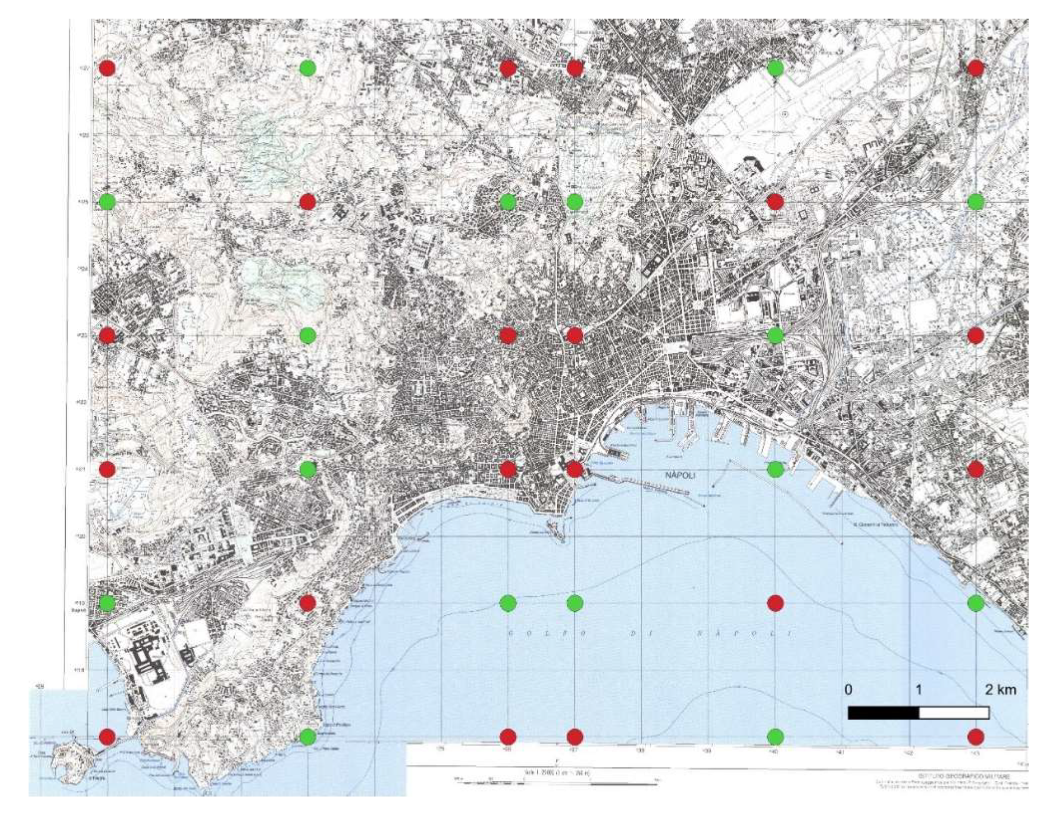
The topographic map is georeferenced by using the software Quantum GIS (QGIS), version 3.10.3. For georeferencing, a coordinate system needs to be set. In this case, the coordinate system is UTM/ED 50 zone 33 N.

In order to georeference this map, affine transformation is applied, using 20 GCPs and 16 CPs, which are both identified as the kilometric grid nodes, as shown in Figure 10.

Statistical values of CP residuals are shown in

Table 1. Statistical values of CP residuals for the topographic map.

Min (m)	Max (m)	Mean (m)	Standard Deviation (m)	RMSE (m)
0.720	10.393	4.414	3.217	5.462

. In consideration of the map scale (1:25,000), the results satisfy the positional accuracy requirement (10 m) while remarking the efficiency of affine transformation that is enough for georeferencing scanned maps.

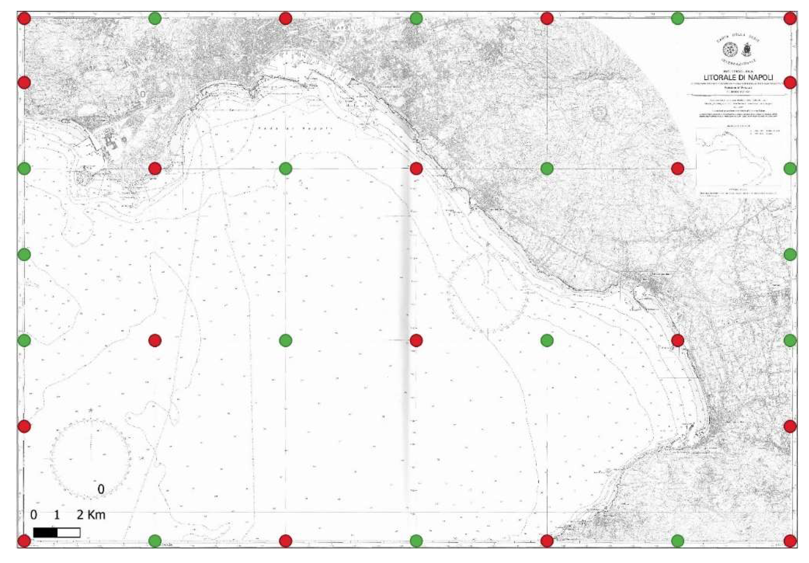
Another georeferencing process occurs for the nautical chart. The coordinate system is now OSPM ED50. A total of 18 GCPs and 16 CPs are used for georeferencing. The points are taken on the geographic grid nodes, as shown in Figure 11.

As for the topographic map, affine transformation is applied. Comparing the resulting OSPM ED50 plane coordinates of CPs with the exact values, the residuals reported in

Table 2. Statistical values of CP residuals for the nautical chart.

Min (m)	Max (m)	Mean (m)	Standard Deviation (m)	RMSE (m)
1.326	9.928	4.917	2.133	5.360

are achieved.

In consideration of the map scale (1:30,000), the results satisfy the positional accuracy requirement (12 m) by remarking on the efficiency of affine transformation.

5.2. Orthorectification of Dataset 3

As far as it concerns the satellite dataset, GeoEye-1 imagery is supplied with a low level correction. Therefore, it is already referred to as a coordinate system, UTM/WGS84 zone 33 N, but the positional accuracy is inadequate to the geometric resolution. However, the low-level correction does not take into account the variability caused by elevation. The dataset is not already orthorectified in the photogrammetric sense, so it presents errors in its geo-localization.

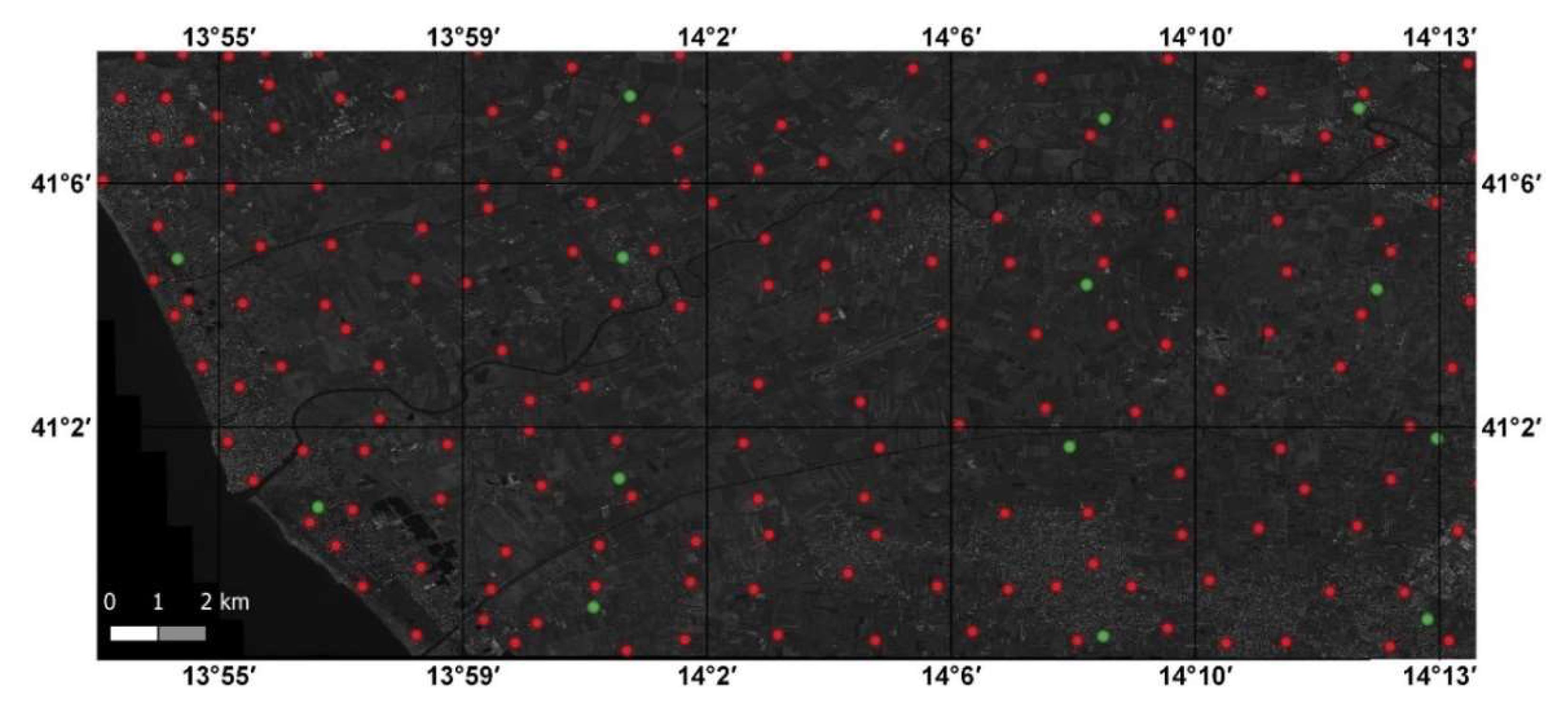
The orthorectification of 181 GCPs with a regular planimetric and altimetric distribution on the GeoEye-1 image set are identified. In order to preserve the original radiometric values, the nearest-neighbor algorithm is used as a resampling method. The planimetric coordinates of GCPs are obtained by orthophotos of the Campania region with 0.20-m resolution instead of the elevations obtained by Digital Elevation Model (DEM) with a cell size of 20 m supplied by IGM (Istituto Geografico Militare). The positional accuracy is tested using 15 CPs identified on the study area in the same way as that for GCPs, as shown in Figure 12.

The orthorectification process is carried out by using the software OrthoEngine—PCI Geomatics. The results are shown in

Table 3. Statistical values of the CP residuals for GeoEye-1 orthorectification.

Min (m)	Max (m)	Mean (m)	Standard Deviation (m)	RMSE (m)
0.241	1.952	0.800	0.429	0.908

.

As reported in literature, good results of orthorectification are achieved for positional accuracy when residuals are minor than compared to 1.5–2 times the pixel size. Considering that the geometric resolution of GeoEye-1 is 0.50 m for the panchromatic image, the results satisfy the positional accuracy requirement (1 m). Therefore, the layer is useful for the CMGIS application at a scale of 1:2,500.

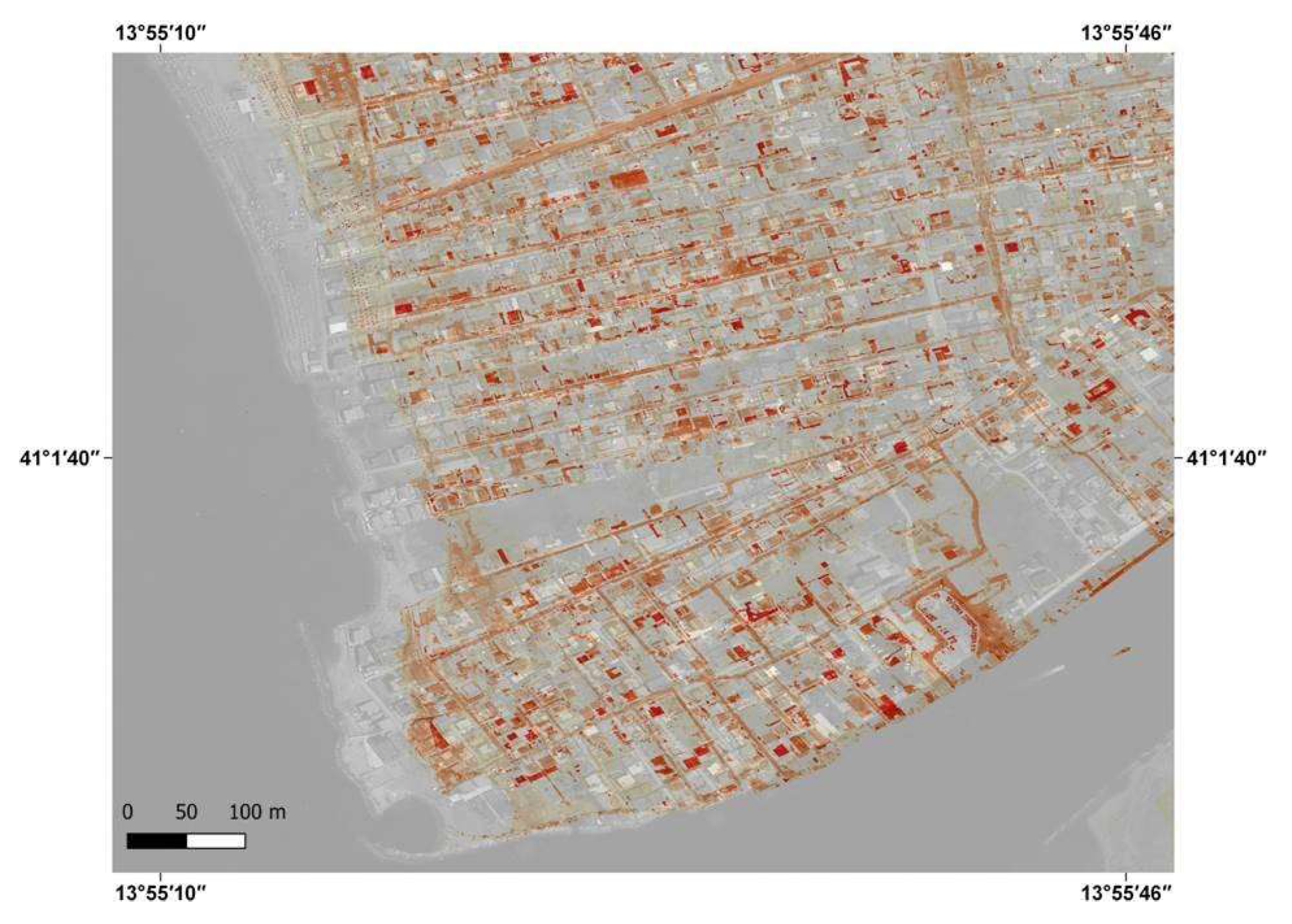
If the orthorectification is not performed, the image results shifted in the South-West direction, as shown in Figure 13.

Actually, the differences in position can be estimated by taking the coordinates of the same object in the two different layers. We use the CPs adopted for orthorectification to evaluate those differences. The statistical values of CP residuals are shown in

Table 4. Statistical values of CP residuals resulting from the ortho-rectified imagery and original imagery comparison.

Min (m)	Max (m)	Mean (m)	Standard Deviation (m)	RMSE (m)
49.142	61.734	57.478	3.912	57.611

.

The results remark the inappropriateness of satellite images presenting low level correction. The use of RPFs permits us to easily enhance the positional accuracy of the dataset by adapting it to the appropriate scale usage in consideration of the pixel size.

5.3. Datum Transformation of Datasets 1, 2, and 6

Datum transformation is necessary for the topographic map (dataset 1), nautical chart (dataset 2), and bathymetric points (dataset 6) because they are all referred to ED50 datum and need to be translated to WGS84.

With regard to the topographic map and the bathymetric points, a datum transformation from UTM ED50/zone 33 N to UTM WGS84/zone 33N is carried out by using the NG. To reduce the transformation datum to a simplified approach based only on the translation in x and y directions, the differences between the corresponding x coordinates as well as the corresponding y coordinates are calculated. Then the average of those differences are considered in order to obtain a unique translation value in each direction (one in the x direction and one in the y direction). For the east coordinates, the translation value is 67.857 m and, for the North coordinates, the value is 193.130 m.

In order to check the effectiveness of this simplified approach to datum transformation, the resulting values of the translation are compared with the exact values of the corresponding points in UTM WGS 84/zone 33 N supplied by NG.

The statistical values of the residuals related to this simplified approach (translation) are shown in

Table 5. Statistical values of the residuals for the East coordinates resulting from datum transformation UTM/ED50 to UTM/WGS84 based on a simplified approach (translation).

Min (m)	Max (m)	Mean (m)	Standard Deviation (m)	RMSE (m)
−3.503	1.696	0	1.736	1.736

and

Table 6. Statistical values of the residuals for the North coordinates resulting from datum transformation UTM/ED50 to UTM/WGS84 based on a simplified approach (translation).

Min (m)	Max (m)	Mean (m)	Standard Deviation (m)	RMSE (m)
−1.384	1.077	0	0.705	0.705

.

To achieve greater precision, roto-translation with a conformal transformation must be applied. The statistical values of the residuals related to roto-translation are shown in

Table 7. Statistical values of the residuals for the East coordinates resulting from datum transformation UTM/ED50 to UTM/WGS84 based on a conformal approach.

Min (m)	Max (m)	Mean (m)	Standard Deviation (m)	RMSE (m)
−0.637	1.158	0	0.553	0.553

and

Table 8. Statistical values of the residuals for the North coordinates resulting from datum transformation UTM/ED50 to UTM/WGS84 based on a conformal approach.

Min (m)	Max (m)	Mean (m)	Standard Deviation (m)	RMSE (m)
−0.748	0.879	0	0.529	0.529

.

The same procedure is carried out for the nautical chart. The average translation values are 0.048504′ for longitude coordinates and 0.061904′ for latitude coordinates. Statistical values of the residuals can be found in

Table 9. Statistical values of the residuals for the longitude coordinates resulting from datum transformation OSPM/ED50 to OSPM/WGS84 based on a simplified approach (translation).

Min (Minutes)	Max (Minutes)	Mean (Minutes)	Standard Deviation (Minutes)	RMSE (Minutes)
−0.00357600	0.00470400	0	0.00255796	0.00255796

and

Table 10. Statistical values of the residuals for the latitude coordinates resulting from datum transformation OSPM/ED50 to OSPM/WGS84 based on a simplified approach (translation).

Min (Minutes)	Max (Minutes)	Mean (Minutes)	Standard Deviation (Minutes)	RMSE (Minutes)
−0.00181600	0.00166400	0	0.00104256	0.00104256

.

The statistical values of the residuals related to roto-translation are shown in

Table 11. Statistical values of the residuals for the longitude coordinates resulting from datum transformation OSPM/ED50 to OSPM/WGS84 based on a conformal approach.

Min (Minutes)	Max (Minutes)	Mean (Minutes)	Standard Deviation (Minutes)	RMSE (Minutes)
−0.00068816	0.00121336	0	0.00054967	0.00054967

and

Table 12. Statistical values of the residuals for the latitude coordinates resulting from datum transformation OSPM/ED50 to OSPM/WGS84 based on a conformal approach.

Min (Minutes)	Max (Minutes)	Mean (Minutes)	Standard Deviation (Minutes)	RMSE (Minutes)
−0.00066310	0.00076868	0	0.00043348	0.00043348

.

As far as the nautical chart is concerned, there are reported values for the transformation of datum provided by the Hydrographic Institute of the Italian Navy (IIMM). In particular, the following values are reported.

• Longitude differences ED50 − WGS84 = 0.05 min.
• Latitude differences ED50 − WGS84 = 0.06 min

The conversion values proposed by IIMM are close to those determined when using NG.

Positional accuracy can, therefore, be compromised if an adequate data transformation is not carried out. The shift between the two datum would be evident, as shown in Figure 14.

The use of the NG assumes great importance in relation to the fact that the GIS software, in this case QGIS, is not very accurate in relation to the transformation of datum. To test the accuracy of the GIS automatic procedure, an analysis is performed on the UTM WGS84/zone 33N coordinates transformed from the same UTM ED50/zone 33N coordinate dataset. Furthermore, in this case, the QGIS results are compared with the NG results. The statistical values of these residuals are reported in

Table 13. Statistical values of the residuals for the East coordinates resulting from datum transformation UTM/ED50 to UTM/WGS84 based on automatic QGIS application.

Min (m)	Max (m)	Mean (m)	Standard Deviation (m)	RMSE (m)
−8.314	−1.874	−4.197	2.084	4.686

and

Table 14. Statistical values of the residuals for the North coordinates resulting from datum transformation UTM/ED50 to UTM/WGS84 based on automatic QGIS application.

Min (m)	Max (m)	Mean (m)	Standard Deviation (m)	RMSE (m)
2.697	5.887	4.206	0.910	4.303

.

The same procedure is repeated for OSPM/ED50 coordinates transformed in OSPM/WGS84 coordinates by using QGIS. The statistical values of the resulting residuals are reported in

Table 15. Statistical values of the residuals for the longitude coordinates that result from datum transformation OSPM/ED50 to OSPM/WGS84 based on an automatic QGIS application.

Min (Minutes)	Max (Minutes)	Mean (Minutes)	Standard Deviation (Minutes)	RMSE (Minutes)
−0.00582000	−0.00138000	−0.00298000	0.00143654	0.00330818

and

Table 16. Statistical values of the residuals for the latitude coordinates resulting from datum transformation OSPM/ED50 to OSPM/WGS84 based on automatic QGIS application.

Min (Minutes)	Max (Minutes)	Mean (Minutes)	Standard Deviation (Minutes)	RMSE (Minutes)
0.00150000	0.00318000	0.00227200	0.00049366	0.00232501

.

Ultimately, the datum transformation can be carried out in alternative ways such as by using simple translation along the x and y axes, introducing roto-translation, and using the automatic mode of the software. The first two approaches require that the user has the appropriate transformation parameters. The third requires no a-priori knowledge. However, although it is easier to apply, the third way provides the worst results. Simple translation improves results compared to the automatic mode, but the best solution is provided by roto-translation. When the translation or roto-translation parameters are not available for a given area, they can be easily calculated with the use of double points. Provided the coordinates in a certain system, the corresponding ones in anther system can be determined by using reliable tools. In the Italian case, a similar tool is the NG.

5.4. Reprojections of Datasets 1, 3, 4, 5, and 6

The Datasets (1)–(6) need to be reprojected. Particularly, Dataset (5) is geo-referred in WGS84 ellipsoidal coordinates while all the others are in the UTM projection. The automatic procedure based on QGIS tools is applicable because OSPM WGS84 is now available. Tests are carried out to evaluate the positional accuracy of reprojection. For Datasets (1)–(5), grid nodes referred to as UTM-WGS84 are submitted to reprojection in OSPM WGS84 and the resulting coordinates are compared to the corresponding ones obtained by the rigorous application of the corresponding equations. In a similar way, for Dataset (5), grid nodes referred to WGS84 ellipsoidal coordinates are submitted to reprojection in OSPM WGS84 and tested.

The statistical values related to the reprojection from UTM WGS84/zone 33 N plane coordinates to OSPM WGS84 are shown in

Table 17. Statistical values of the residuals for the East coordinates after reprojection from UTM/WGS84 to OSPM/WGS84.

Min (m)	Max (m)	Mean (m)	Standard Deviation (m)	RMSE (m)
0	0.001	0.001	0	0.001

and

Table 18. Statistical values of the residuals for the North coordinates after reprojection from UTM/WGS84 to OSPM/WGS84.

Min (m)	Max (m)	Mean (m)	Standard Deviation (m)	RMSE (m)
0.013	0.014	0.014	0	0.014

. Analogous results for the reprojection from WGS84 ellipsoidal coordinates to OSPM WGS84 are shown in

Table 19. Statistical values of the residuals for the East coordinates after reprojection from WGS84 ellipsoidal coordinates to OSPM/WGS84.

Min (m)	Max (m)	Mean (m)	Standard Deviation (m)	RMSE (m)
−0.0002	−0.0002	−0.0002	0	0.0002

and

Table 20. Statistical values of the residuals for the North coordinates after reprojection from WGS84 ellipsoidal coordinates to OSPM/WGS84.

Min (m)	Max (m)	Mean (m)	Standard Deviation (m)	RMSE (m)
−0.0004	0.0005	0	0.0003	0.0003

.

The resulting errors are very small (practically traceable), so we can assert that, due to the correct definition and introduction of the OSPM projection in the software available options, the reprojection does not present any loss of positional accuracy.

6. Conclusions

In order to build a CMGIS, it is necessary to integrate heterogeneous data. In this study, different datasets are considered in order to deal with different and exemplary cases and choose the best solutions.

Dataset 1 needs to be geo-referenced in the UTM ED50/zone 33 N system to undergo datum transformation in WGS84 and to be re-projected into the OSPM WGS84. Dataset 2 is geo-referenced in geographic coordinates with datum ED50. It also undergoes a transformation of datum into WGS84 and is, therefore, reprojected into an OSPM WGS84. Dataset 3 is orthorectified. It must not undergo any transformation of datum because it is in the UTM WGS84/Zone 33 N system. Therefore, a reprojection in the OSPM WGS84 is necessary. Dataset 4 is georeferenced in UTM WGS84/Zone 33 N and requires only the OSPM WGS84 reprojection. Dataset 5 is georeferenced in WGS84 ellipsoidal coordinates and requires only the OSPM WGS84 reprojection. Dataset 6 is georeferenced in UTM ED50/Zone 33 N and requires datum transformation in WGS84 and the OSPM WGS84 reprojection.

Georeferencing a scanned map by assigning it a datum and a projection is a simple operation if performed in a GIS. The accuracy of the georeferencing process is adequate. You only need to know how to choose the GCPs in the right way by using the geographic grid or the kilometric grid nodes and their values in order to achieve a degree of accuracy at least equal to that of the chart. RMSE values for both the topographic map and nautical chart confirm that good results can be achieved by using the software georeferencing tool in the correct way.

Orthorectification is necessary for VHR satellite images because they should be acquired with a low level of positional accuracy. The necessary tools are generally not available in GIS, and, therefore, specific software needs to be used. By applying RPFs, good results are achieved, as testified by the RMSE value that is less than twice the image of the cell size.

On the fly datum transformations available in GIS software are usually imprecise because, based on unspecified parameters, a global but not regional order are required in a CMGIS. Datum transformations necessitate the estimation of local parameters. Therefore, double points are correctly estimated. In our case, the double points are defined starting from a grid in a specific datum (ED50) in which node coordinates in another datum (WGS84) are derived from a very reliable source, such as NG. Double points permit us to define the four parameters of datum transformation (one rotation, two translations, one scale factor) for the study area. A simplified approach based on a translation parameter application is less accurate but supplies better results for our area than the automatic transformation available in QGIS software.

While the use of global Mercator charts in GIS is recurrent, since this is the most used chart for navigation, the same cannot be said for the OSPM. In particular, for an area of limited extension such as that concerning the Campania coasts and the stretch of sea in front of them, it is useful to apply the Mercator chart with a standard parallel at 40.75° N. This projection may be not be present in the software. Therefore, it needs to be previously set in order to guarantee the feasibility of georeferencing and reprojection operations.

When the input and output projections are corrected, defined, and available, the reprojection operation has a good degree of accuracy. This is because the software takes the coordinates of the starting projection, returns to the ellipsoid by transforming them into geographical ones, and projects them in the new projection. It is clear that, if the output projection is not among the available ones, as for the OSPM, it is not possible to carry out the reprojection.

The aspects described in this article are recurrent in CMGIS and the adopted solutions are exportable in similar situations as well as easily adaptable to analogous cases. In the presence of a different projection (i.e., Gauss-Boaga) or datum (i.e., Roma40), the approach is similar and requires the correct parameters.