Study on the Influence of Temperature on the Temporal and Spatial Distribution Characteristics of Natural Cavitating Flow around a Vehicle

Abstract

Cavitation involves complex multiphase turbulence and has important research significance. In this study, the Schnerr–Sauer cavitation model was used to model cavitation, and the detached-eddy simulation (DES) method was used to calculate the unsteady natural cavitating flow. The predicted results are in good agreement with experimentally measured cavity evolution and pressure values, demonstrating the effectiveness of this numerical method. Low temperature causes changes in the properties of water. The density of water at 0° is 999.84 kg/m³ and the density of water at 25° is 997.04. Cavitation evolution and shedding are analyzed at temperatures of 0 °C and 25 °C. The results showed that lower temperature increased the frequency of cavitation and enhanced pressure pulsation. At the same time, low temperature also increases the frequency of cavity shedding and shortens the cycle. In addition, based on the Ω method, the difference between vortex dynamics at various temperatures was studied, and it was found that different cavity stages showed different vortex structure characteristics, and lower temperature would aggravate the change of wake vortex structure. At the same time, the analysis of the turbulence characteristics in the downstream of the cavity shows that the lower temperature reduces the velocity pulsation and reduces the turbulence integral scale. At the end of the model, large-scale pulsations are transformed into small-scale pulsations.

1. Introduction

Cavitation usually occurs when the pressure in a liquid stream drops below the local saturated vapor pressure, causing cavities to be generated at the internal or liquid–solid interface [1,2]. Cavitating flows are typically unsteady and exhibit phase changes, turbulence, and multi-scale vortices. Such flows occur in various fluidic machines, including liquid rocket engines, turbines, marine propellers, and hydrofoils. Cavitation can cause serious problems in fluid machinery, such as pressure fluctuations, noise, vibration, and corrosion. Therefore, cavitating flows continue to be widely studied [3,4,5,6].

To date, many experimental and numerical studies have investigated the flow characteristics of cavitation [7,8,9,10]. Knapp [11] observed and analyzed cloud cavitation flow and pointed out that the re-entrant flow from the closed cavity position is the cause of cloud cavitation ruptures. Reissman et al. [12] studied cloud-like cavitation around an oscillating hydrofoil using high-speed cameras and pressure sensors and investigated the mechanism of transient pressure pulses near the detached cavitation. Passandideh-Fard and Roohi [13] used an improved volume-of-fluid (VOF) method to capture the gas–liquid interface of a two-dimensional cavitating flow field. It was found that the improved VOF method offers higher calculation efficiency and accuracy. Ganesh et al. [14] studied how wedge-shaped cavitation evolved into cloud cavitation through wedge geometric model experiments. They found two types of cavity shedding mechanisms in the cavitating flow field: the re-entrant jet mechanism and the shock wave mechanism. The occurrence and collapse of cavitation are periodic. This periodic pressure shock will change the dynamic characteristics of the flow field, also causing strong vibration and noise. In addition, the re-entrant jets and shock waves formed during cavitation collapse can cause high-pressure pulsations on the surface of the material [15,16,17]. Wang et al. [18] performed numerical calculations of the transient characteristics of cloud cavitating flows and shock wave dynamics. They reported several valuable results regarding the influence of water/vapor compressibility in the cavitation instabilities and the relation between cavity development and pressure fluctuations. Ji et al. [19] conducted a numerical study of the cavitating flow structure around a twisting hydrofoil. Three flow characteristics on the suction side of the twisted hydrofoil were analyzed, and the vorticity transport equation in the variable density flow was used to illustrate the effect of cavitation on the vorticity distribution. De et al. [20] studied the structure of the unsteady cavitation flow on the hydrofoil through appropriate orthogonal decomposition (POD) and fast Fourier transform (FFT) techniques, focusing on analyzing the effects of DCM and PBE models on three different cavitation methods (bubble cavitation, cloud cavitation and supercavitation). Kadivar et al. [21] applied the passive flow control method to numerically and experimentally study the unsteady cavitation fluctuation around the semicircular front edge plate. The research found that the passive control method can better prevent the development of the attachment cavity’s spanwise instability and mitigate the large cavity structure. Timoshevskiy et al. [22] used PIV technology to analyze the cavitation state from the velocity field of the 2D symmetric hydrofoil cavitation under four velocity conditions. The data showed that the turbulence distribution and turbulence distribution of turbulence changed significantly with the development of cavitation. In particular, the behavior of the average speed and the most probable speed unexpectedly seems to be different.

The physical properties of fluids are related to temperature, and changes in fluid properties further affect the evolution of the cavity and the flow field [23,24]. Typical thermo-fluids include cryogenic fluids, refrigerants, fluoroketone, and high-temperature water. Hall et al. [25] conducted comprehensive experiments with four cavitation test models in water and Freon 113 at different inlet speeds and temperatures. Cervone et al. [26] conducted experiments in water around NACA0015 hydrofoils at different cavitation numbers and free flow temperatures (298–343 K) to study the characteristics of cavitation instabilities. Franc et al. [27] studied the cavitation instability of the refrigerant R-114 at three different temperatures and proved that a higher reference temperature delayed the occurrence of blade cavitation. Petkovšek and Dular [28] conducted experimental research on the temperature field of cavitation in hot water and measured the temperature dynamics under various operating conditions. Chen et al. [29] studied the fluoroketone phase transfer process by evaluating the temperature and speed of various free flows. These numerical studies have provided accurate predictions and insights into the characteristics of cavitating flow in thermosensitive fluids. Sun et al. [30] studied an unsteady cavitating flow on the NACA0015 hydrofoil in a fluoroketone thermosensitive fluid, with particular emphasis on the cavitation shedding dynamics. Studies have shown that the temperature of the hydrofoil increases and decreases under certain thermal conditions. Thermal effects suppress cavitation and have the potential to reduce pressure pulsation peaks. The current research on temperature mainly focuses on low-temperature fluids. In a low-temperature water environment, the mechanism of changes in the cavity evolution and vortex structure is still unclear. Wang et al. [31] used OpenFOAM to perform a 3-D numerical simulation of the transient sheet/cloud cavitation flow around a Clark-Y hydrofoil. The results show that the compressible method can predict the reentrant jet dynamics well. The velocity divergence comes from the compressibility and mass transfer of the cavitation two-phase fluid, and also depends on the fluid density. At the same time, the temperature and density changes in different cavitation structures are given.

In cavitating flow simulations, the selection of the turbulence model plays an important role, and the numerical prediction results produced by different turbulence models will typically vary [32,33,34,35]. At present, the Reynolds-averaged Navier–Stokes (RANS) method is very popular in practical engineering, and most numerical simulations use the RANS method for cavitating flow calculations. Combining the VOF model and the k-ω SST turbulence model, An et al. [36] performed a numerical simulation of the supercavitating flow field formed on the submerged body of ground vehicles during the artificial ventilation process and analyzed the influence factors of resistance. Despite its good stability, reasonable computational cost, and acceptable accuracy, RANS overpredicts the turbulent eddy viscosity. In recent years, with the development of computer technology, the large-eddy simulation (LES) framework has increasingly been used to simulate cavitating flows [37,38,39,40]. Huang et al. [41] used the LES method to numerically study the cavitating flow on the flexible NACA66 hydrofoil and analyzed the vibration and cavitation vortex structure caused by the flow. The results show that the change trend of the cavity is consistent with the evolution of the vortex, and the vortex gradually increases in the wake. LES can predict the unstable characteristics of the flow [42,43], but requires a very fine mesh and small time steps. Therefore, the computational cost of the numerical simulations is very high. As a compromise, separation vortices have been widely used in large-separation unsteady flows in recent years. Kunz et al. [44] simulated an unsteady cavitating flow on a hydrofoil using the RANS and detached-eddy simulation (DES) methods, comparing the evolution of the cavity and the changes in lift and drag. The separation vortex approach combines the advantages of RANS and LES: the RANS method is used for simulating the near-wall area to reduce the grid size and calculation time, with the LES method used to simulate the area away from the wall to capture large-scale separated flows [45,46,47].

Although a lot of encouraging work has been conducted on cavitation, further research is still needed. Therefore, this article introduces a numerical study of rotating bodies at two temperatures. What is different from the past is that we pay attention to the influence of low temperature water environment on the temporal and spatial characteristics of cavitation flow. The main purpose is to study the effect of changes in fluid physical properties on cavitation. Section 2 introduces the numerical simulation models, including the basic governing equations, cavitation models, turbulence models, and verification of the numerical methods. Section 3 discusses and analyzes the influence of temperature on the cavity evolution, period, pressure fluctuations, vortex structure, and turbulence scale. Finally, Section 4 summarizes the results of this study and states the main conclusions.

2. Mathematical Formulations and Numerical Methods

2.1. Governing Equations

In this study, the Euler multiphase flow model was used to simulate natural cavitating flow. By solving a set of momentum equations over the entire watershed and tracking the volume fraction of each phase in the finite volume of each fluid, the two-phase immiscible flow was simulated. The mixing density is expressed as:

$$\rho ={\alpha }_l{\rho }_l+\left(1-{\alpha }_l\right){\rho }_v$$

(1)

where $\rho$ is the mixture density and ${\alpha }_l$ represents the water volume fraction.

For the multiphase cavitating flow process, the mass and momentum of the movement of matter are conserved. This is expressed as follows:

$$\frac{\partial \left({\rho u}_i\right)}{\partial t}+\frac{\partial \left({\rho u}_i{u}_j\right)}{\partial x_j}=0$$

(2)

$$\frac{\partial \left(\rho u_i\right)}{\partial t}+\frac{\partial \left(\rho u_i{u}_j\right)}{\partial x_j}=-\frac{\partial p}{\partial x_i}+\frac{\partial }{\partial x_j}\left(\mu \frac{\partial u_i}{\partial x_j}\right)$$

(3)

where p is the pressure and u represents velocity; the subscripts i and j indicate the direction of the velocity component.

2.2. Detached-Eddy Simulation Model

The standard Spalart–Allmaras model defines the turbulence scale as the distance to the nearest wall, d. The original DES model proposed by Spalart et al. [48] was modified using the length scale:

$$\tilde{d}=\min \left(C_{DES}\Delta ,d\right)$$

(4)

where C_DES is a calibrated constant that functions similar to the Smagorinsky constant in the sub-grid stress model. ∆ is based on the largest dimension of the grid cell:

$$\Delta \equiv \max \left(\Delta x,\Delta y,\Delta z\right)$$

(5)

Based on the shear-stress transport (SST) model, Menter et al. [49] developed a two-equation SST–DES method and modified the dissipation term of the k equation. The model equation is:

$$\frac{\partial k}{\partial t}+\frac{\partial \left(u_{j}k\right)}{\partial x_j}=\tilde{G}-{\beta }^{*}k\omega F_{DES}+\frac{\partial }{\partial x_j}\left[\left(v+{\alpha }_k{v}_t\right)\frac{\partial k}{\partial x_j}\right]$$

(6)

where F_DES is the scale factor of the vortex separation method, given by:

$$F_{DES}=\max \left[\frac{L_t}{C_{DES}\Delta }\left(1-F_S\right),1\right]$$

(7)

and the calculated turbulence length scale L_t is:

$$L_t=\frac{\sqrt{k}}{{\beta }^{*}\omega }$$

(8)

$${\mathsf{\Delta }}_1=\sqrt[3]{\mathsf{\Delta }x\mathsf{\Delta }y\mathsf{\Delta }z}$$

(9)

2.3. Schnerr–Sauer Cavitation Model

The Schnerr–Sauer cavitation model is composed of transport equations. This model is obtained by simplifying and improving the Rayleigh–Plesset cavity dynamics equation (Rayleigh, [50]; Plesset, [51]). The self-simplified Rayleigh–Plesset equation can be expressed as:

$$\frac{P_V-P}{P_l}=R\frac{d^2{R}_B}{d{t}^2}+\frac{3}{2}{\left(\frac{d{R}_B}{dt}\right)}^2+\frac{2\xi }{{\rho }_{l}R}$$

(10)

where P_V is the saturation pressure at the local temperature, P is the pressure around the cavity, R_B denotes the bubble radius, and ξ is the surface tension between liquid and vapor.

Ignoring second-order terms and surface tension, this equation can be simplified to:

$$\frac{d{R}_B}{dt}=\sqrt{\frac{2}{3}\frac{P_V-P}{{\rho }_l}}$$

(11)

The processes of evaporation and condensation are expressed by inserting a source term into the transmission equation to describe the phase transition rate. The Schnerr–Sauer model is used as the cavitation model [52]. The transfer equation is:

$$\frac{\partial \left({\rho }_v{\alpha }_v\right)}{\partial t}+\frac{\partial \left({\rho }_v{\alpha }_v{u}_j\right)}{\partial x_j}={\dot{m}}^{+}-{\dot{m}}^{-}$$

(12)

where ${\alpha }_v$ is the vapor volume fraction. The source terms ${\dot{m}}^{+}$ and ${\dot{m}}^{-}$ denote evaporation and condensation, and can be written as:

$${\dot{m}}^{+}=\frac{{\rho }_v{\rho }_l}{\rho }{\alpha }_v\left(1-{\alpha }_v\right)\frac{3}{R_b}\sqrt{\frac{2}{3}\frac{\max \left(P_v-P,0\right)}{{\rho }_l}}$$

(13)

$${\dot{m}}^{-}=\frac{{\rho }_v{\rho }_l}{\rho }{\alpha }_v\left(1-{\alpha }_v\right)\frac{3}{R_b}\sqrt{\frac{2}{3}\frac{\max \left(P-P_v,0\right)}{{\rho }_l}}$$

(14)

where ${\dot{m}}^{+}$ is the evaporation term, ${\dot{m}}^{-}$ is the condensation term, and $P_v$ is the saturation vapor pressure at the local temperature. $R_b$ is the cavity radius, which is given by:

$$R_b={\left(\frac{{\alpha }_v}{1-{\alpha }_v}\frac{3}{4\pi }\frac{1}{N_b}\right)}^{\frac{1}{3}}$$

(15)

where N_b is the density of cavity number. According to Schnerr and Sauer [52], N_b = 10¹³.

2.4. Numerical Setup

Figure 1 shows a schematic diagram of the computational geometric model. It has a conical axisymmetric body with a diameter of D = 40 mm and a length of L = 335 mm. The length of the head is 19 mm, the length of the cylinder is 316 mm, and the angle between the cone section of the head and the cylinder is 45°. Four pressure monitoring points are set up to verify the numerical method and analyze the results. P1 is 100 mm from the model head, P2 is 12 mm from P1, P3 is 8 mm from P2, and P4 is 22 mm from P3. The P2 and P4 points correspond to the experimental monitoring points to verify the validity of the numerical simulation, and the P1 and P3 points, respectively, detect the pressure pulsation inside the cavity and the drop position.

Figure 2 shows the size of the calculation domain around the calculation model. The relative position of the calculation model in the calculation domain is also shown. The distance between the entrance to the calculation domain and the front end of the model is 15D, the distance between the exit and the rear edge of the model is 20D, and the distance between the upper wall and the lower wall is 10D. The entrance to the calculation domain is set as a velocity inlet, the surroundings are set as symmetry planes, and the outlet is assigned a pressure outlet boundary condition. The entry to the calculation domain is set to an inflow velocity of V_∞ = 30 m/s, giving a Reynolds number of Re = 8.9 × 10⁶. The cavitation number changes according to the temperature (Brennen, [53]), and is defined as:

$$\sigma =\frac{P-P_v}{0.5{\rho }_l{v}_{\infty }^2}$$

(16)

To study the characteristics of turbulence at different temperatures, detection surfaces were set up inside the cavity and downstream of the trailing edge of the model, as shown in Figure 3a. The detection surface is composed of 13 evenly spaced concentric circles, with 90 monitoring points distributed on each circle. Figure 3b shows the rear view of the monitoring surface.

Figure 4 shows the calculation grid. To capture the detailed features of unstable flow, the surface of the model has a prism layer and the front end of the model has a higher resolution to better capture the cavitation evolution. In each time step, performing too many iterations will increase the calculation time without noticeably improving the accuracy, whereas performing too few iterations may lead to poor convergence and inaccurate calculations. In the simulations, 10 iterations were performed in each time step to ensure a suitable balance between accuracy and efficiency. The grid contained approximately 8 × 10⁷ cells and the calculated y+ was less than 1.

2.5. Numerical Method Validation

The experiments mainly investigated a circulating high-speed ventilated cavitation in the water tunnel of the Harbin Institute of Technology. The experimental system has been described in detail in a previous article (Zhang et al. [54]). In the process of numerical simulation, a steady field is given to the flow field. After the flow field is stable, the cavitation model is turned on to simulate the evolution of the cavity. In the test conditions considered in this study, the working pressure was 68.4 kPa, the flow velocity of the water tunnel is 10.21 m/s, and the cavitation number was 0.62. Figure 5a,b compare the instantaneous cavity shape in the experiments and the numerical predictions. At the same time, Figure 5c illustrates the volume fraction distribution of the XOY plane. At t₀ + 6.7 ms, at the front end of the cavity, a gap appears at the shoulder of the model, as shown in Figure 6a,b. From t₀ + 6.7 ms to t₀ + 13.4 ms, large-scale shedding occurs over the entire cavity and moves downstream. This is the main shedding process and causes a large pressure pulsation downstream. At t₀ + 20.1 ms, the large-scale shedding ends, and the front-end cavitation develops again. At t₀ + 26.8 ms, the length of the cavity is the same as at t₀. As shown in Figure 5c, there is a gap at the shoulder of the cavity at t₀ + 6.7 ms. At t₀ + 13.4 ms, under the influence of the re-entrant flow, a large cavity detaches from the entire cavity on the main body. At t₀ + 20.1 ms, the shed cavity moves downstream and gradually collapses. The results of the experiment are in good agreement with those from the simulations.

Figure 6 compares the experimental and numerical pressure curves at monitoring points P2 and P4. The large-scale shedding of the cavitation bubbles moves downstream. The pressure fluctuations are obvious, first decreasing and then increasing as the cavitation bubbles pass. These results verify that the numerical method proposed in this paper can effectively predict the flow field evolution and pressure pulsation of cavitating flow.

In this study, we use STAR-CCM+ to conduct numerical simulation research; the time step was set to $\Delta t=2.5\times {10}^{-5}$ s so that the Courant number was less than 1 at every position in the computational domain, thus ensuring good convergence. The numerical simulations were based on the finite volume method, and the VOF model adopted a second-order implicit scheme. The governing equations were subjected to second-order discretization in space. The split solver based on the SIMPLE algorithm was used to handle the coupling between the velocity and the pressure.

3. Results and Discussion

3.1. Cavity Evolution and Pressure Pulsation

Figure 7 shows the typical cavity morphology with a water volume fraction of 0.8 at 16 points during the evolution process at 0 °C and 25 °C. The initial position of natural cavity is at the position of the dotted line a. From t₀ to t₀ + 6.0 ms, the volume of the cavitation bubble increases to its maximum size. With the generation of the re-entrant jet, the cavity downstream gradually shedding. The volume of the cavitation bubble gradually decreases until it collapses to the position where the initial cavitation bubble is generated. At t₀ + 6.0 ms, the cavitation length is greater in the 25 °C flow than in the 0 °C flow, and a vortex structure is generated at the tail. At t₀ + 7.5 ms, the shedding of the vortex structure reduces the cavitation size, and we can determine that the collapse rate of the 0 °C cavitation bubble is faster than in the 25 °C case by comparing dotted lines b and c. At t₀ + 21.0 ms, the 0 °C cavitation bubble has collapsed to its smallest volume, and the system has entered the next cycle. The 25 °C cavitation bubble reaches its minimum size at t₀ + 22.5 ms, which is about 1.5 ms slower than at the lower temperature. The density of water at 0 °C is 999.84 kg/m³ and the density of water at 25 °C is 997.04 kg/m³. The saturated vapor pressure at 0 °C is 611 Pa, whereas that at 25 °C is 3169 Pa. The cavitation number of the 25 °C flow is 0.328, and that in the 0 °C case is 0.333. Therefore, the void volume at 25 °C is greater than that at 0 °C. This indicates that a lower temperature increases the instability of cavitation bubbles, accelerates the internal phase transition rate of the cavity, and shortens the evolution period.

To analyze the evolution of cavitation bubbles, Figure 8 shows the changes in cavity volume at the two temperatures. The volume of the cavity changes periodically and oscillates within a certain interval. As the cavity collapses and sheds, the volume of the cavity reaches its minimum value, from which point it begins to grow to its maximum volume once again. Interestingly, the volume change of cavitation bubbles at 25 °C is smoother than at 0 °C, and the volume change in each cycle is also larger. In some periods, the maximum volume of the 0 °C case exceeds the void volume of the 25 °C case. The average volume of the cavity at 0 °C is 1.41 × 10⁻⁴ m³, compared with 1.43 × 10⁻⁴ m³ at 25 °C. The average hole volume at 25 °C is slightly larger than that at 0 °C and there are a greater number of holes. This shows that the lower temperature makes the cavity smaller and accelerates the collapse and shedding processes.

Figure 9a shows the pressure change at two positions at the two temperatures. The pressure change is also periodic. When the cavity reaches position P1, the minimum pressure at each temperature is the saturated vapor pressure. With the collapse and shedding of the cavity bubbles, the pressure fluctuates violently. When the shedding cavity moves to position P3, pressure pulsations can be detected, and the pulsation period is the same as the cavity collapse and shedding period. At the two points, the average pulsation pressure in the 0 °C case is higher than in the 25 °C case, indicating that the pressure pulsations caused by cavitation are more obvious at lower temperatures. This is because the saturated vapor pressure at 0 °C is 611 Pa and that at 25 °C is 3169 Pa. At the same flow rate, the 25 °C cavity is more stable, shedding and collapsing more smoothly, than in the 0 °C case, demonstrating the effect of the pressure pulsations on the shedding and collapse processes. Figure 10 shows the power spectral density (PSD) frequency distribution diagram at pressure detection points P1 and P3 (sampling frequency is 0–2.5 × 10⁴.). The main frequency of natural shedding at 0 °C is 50.0 Hz, compared with 45.8 Hz at 25 °C. It proves that low temperature increases the shedding frequency, that is, the cycle of cavitation evolution is shortened, and the cavitation evolution is intensified, which also corresponds to the result in Figure 8.

3.2. Vortex Structure Characteristics

Turbulence produces a large number of vortex structures with different scales and strengths. These vortex structures play a key role in the generation and maintenance of turbulence and are important in the analysis of cavitation problems. Therefore, it is of great significance to analyze the vortex structure. The third-generation Ω method (Liu [55]) for vortex identification offers enhanced vortex recognition without the need to adjust the threshold according to the flow. Here, the vorticity represents the curl of the velocity:

$$\mathit{\omega }=\nabla \times V$$

(17)

We can decompose the velocity gradient tensor as follows:

$$\nabla V=\mathit{A}+\mathit{B}=\frac{1}{2}\left(\nabla V+\nabla V^T\right)+\frac{1}{2}\left(\nabla V-\nabla V^T\right)$$

(18)

where A is the strain rate tensor, $\mathit{A}=\frac{1}{2}\left(\nabla V+\nabla V^T\right)$, B is the rotation tensor, $\mathit{B}=\frac{1}{2}\left(\nabla V-\nabla V^T\right)$, ${\Vert \mathit{A}\Vert }_F$ ${\Vert \mathit{B}\Vert }_F$ are the Frobenius norm of the matrix, and $\epsilon$ is the correction value:

$$\epsilon ={\epsilon }_c\ast {\left(b-a\right)}_{max}$$

(19)

$$b={\Vert \mathit{B}\Vert }_F^2$$

(20)

$$a={\Vert \mathit{A}\Vert }_F^2$$

(21)

where ${\epsilon }_c={10}^{-7}$ is an empirical constant (Liu et al. [55]). Ω represents the ratio of the vorticity of the rotating part to the total vorticity, which is expressed as

$$\Omega =\frac{{\Vert \mathit{B}\Vert }_F^2}{{\Vert \mathit{A}\Vert }_F^2+{\mathit{B}}_F^2+\epsilon }$$

(22)

Figure 11a shows the vortex structure at the two temperatures during the development stage of the cavity. A strong vortex structure can be found on the surfaces of the two cavities. As the cavity grows, some vortex structures become attached to the surface of the cavity. At both temperatures, the Ω value inside the cavity zone is smaller than that outside the cavity. Inside the cavity, the shearing effect is equivalent to the rotation, while the rotation effect on the surface of the cavity indicates that there is strong rotational movement in this area. As shown by the black dotted line, a strong vortex structure is concentrated at the tail of the model, and the vortex structure is the same at the two temperatures. In the wake area, a large number of linear vortex structures are produced, and these are stronger in the 0 °C case than in the 25 °C case. The change period of 0 °C cavity is faster than that of 25 °C cavity, so the frequency of 0 °C cavity generation and shedding is greater, and a large number of vortex structures move to the wake region. As a result, the 0 °C vortex structure in the wake region is stronger than the 25 °C vortex structure.

Figure 11b shows the vortex structure at the two temperatures at the stage of cavity stability. The vortex structure attached to the surface of the cavity has disappeared, and a strong vortex structure has appeared inside the cavity. The vortex structure at 0 °C is stronger than that at 25 °C. Due to the generation of the back jet, a large amount of vortex motion appears inside the cavity. The 0 °C cavity is more unstable, and its shedding frequency is faster, leading to the stronger vortex structure and the shedding of the next stage of a cavity. At the stage of cavity stability, no vortex shedding occurs and there is no disturbance in the wake region. Therefore, the linear vortex structures in the wake region are the same at both temperatures.

Figure 11c shows the stage of cavity shedding. Several vortex structures are attached to the surface of the cavity, but the vortex structure is weaker than during the cavity development stage. The vortex structure attached to the rear wall of the model is stronger than in the first two stages. This vortex structure is larger in the 0 °C case than at 25 °C. At low temperatures, the vortex structure on the model wall is enhanced. The cavity breaks and sheds, and a large number of vortices move along the wall surface wake. The cavity shedding is faster at 0 °C than at 25 °C, so the wall vortex structure in the back section of the model is stronger at 0 °C.

Comparing the wake field of the three stages, it is found that the vortex structure changes significantly at 0 °C, especially during the development of cavity, and the tail vorticity exhibits a divergent trend. At 25 °C, the overall wake field vortex structure changes more smoothly, although the scale of the vortex structure is larger than at 0 °C. This is because the cavity shedding frequency is lower at 25 °C than at 0 °C, so the vortex structure has a large scale and a small overall strength.

Figure 12 compares the vortex structures produced in three-dimensional natural cavitation evolution at 0 °C and 25 °C. Due to the growth and shedding of the cavity, the vortex structure is always attached to the non-cavitated area of the rear wall of the model, and the scale varies with time. At t₀ + 0 ms, there are many linear vortex structures in the wake field. The vortex structure is stronger at 0 °C than at 25 °C, which is the same conclusion as for Figure 11a. The volume of the cavity has increased at t₀ + 10 ms, resulting in a smooth Ω isosurface in the cavity head and a small velocity gradient, indicating laminar flow. The re-entrant jet causes the flow to undergo a rapid laminar-turbulent transition in the closed position of the cavity, forming a series of vortex structures. These vortex structures move with the direction of the incoming flow and develop into a series of ring-like vortices. At this moment, due to the closure and shedding of the cavity, an annular vortex structure appears in the latter part of the model at 0 °C and at the position of the cavity shedding at 25 °C. As the vortex structure moves downstream, at t₀ + 15 ms, the tail end presents an obvious annular vortex structure. According to the cavity evolution process, the cavity shedding frequency is faster at 0 °C than at 25 °C. Therefore, there is a time difference between the vortex structures at the two temperatures. In general, the vortex structure scale is smaller at 0 °C than at 25 °C. However, there are more vortex structures at the lower temperature, especially in the wake field area of the model.

3.3. Analysis of Turbulence Intensity and Integral Scale

Turbulence characteristics are important to the evolution of cavitation. To study the effect of temperature on the turbulence of natural cavitation and the turbulence integral scale, we established detection surfaces inside the cavity and downstream of the cavity shedding at the two temperatures. The turbulent flow characteristics considered in this paper are based on the assumption of random stationary flow. The time series of the x-axis velocity at time t is used to find the time average. The axial pulsation velocity of the corresponding point can be expressed as:

$$u_x^{\prime }\left(t_j\right)=u_x\left(t_j\right)-\overline{u_x}$$

(23)

The turbulence intensity is expressed as:

$${\epsilon }_x=\frac{{\left[\frac{1}{N-1}{{\displaystyle \sum }}_{j=1}^N\Delta u_x^2\left(t_j\right)\right]}^{\frac{1}{2}}}{U_{ref}}$$

(24)

where U_ref is the flow speed at infinity and ${\epsilon }_x$ is the turbulence intensity in the x-direction.

Figure 13a shows a schematic diagram of the two-dimensional turbulence intensity inside the cavity at the two temperatures. The inside of the cavity exhibits a high degree of turbulence, while the boundary layer area near the model wall has a lower level of turbulence. Due to the violent phase change process in the cavity, the water is transformed into vapor and the velocity changes, which is characterized by higher turbulence intensity and strong instability. Figure 13b shows the three-dimensional turbulence intensity inside the cavity at the two temperatures. The inside of the cavity again exhibits a high degree of turbulence, while the boundary layer area near the model wall shows a lower degree of turbulence. A violent phase transition process occurs inside the cavity. Due to the cavitation effect, the water transforms into vapor and the velocity changes. Therefore, it is characterized by high turbulence intensity and strong instability. It can be seen that the turbulence intensity at 25 °C is 0.3 and that at 0 °C is 0.28, a decrease of approximately 6%. Furthermore, under low-temperature conditions, the internal phase change in the cavity is violent and the cavity becomes unstable.

Figure 14a shows the two-dimensional turbulence intensity of the wake field at the two temperatures. The higher-turbulence area is mainly concentrated in the tail flow field, and its radius is the same as the model radius. This flow phenomenon occurs because the velocity of the flow field in the tail region of the model is small, whereas the velocity on both sides is large. When the two velocities meet in the wake field, a large velocity pulsation occurs. Figure 14b shows the three-dimensional turbulence intensity at the downstream cavity shedding position. The turbulence intensity at 25 °C is 0.175, whereas that at 0 °C is 0.15, a reduction of 14%. Compared with the inside of the cavity, the turbulence intensity is significantly reduced at both temperatures. This is because, as the cavity sheds, the vortex structure is gradually formed and the turbulent dissipation rate increases, causing the turbulent kinetic energy to be converted into heat energy. This is manifested as an overall decrease in turbulence intensity. The vortex structure sheds at both temperatures, and so the turbulence intensity decreases even more.

The turbulence integral scale is the size of the vortex scale in the turbulent pulsation. According to Taylor’s hypothesis (Piomelli et al. [56]), the axial turbulence integral scale can be expressed as:

$$R_S\left(\tau \right)=\underset{N\to \infty }{\lim }\frac{1}{N}{\displaystyle \sum }_{j=1}^N\Delta u_x\left(t_j\right)\Delta u_x\left(t_j+\tau \right)$$

(25)

$$\Lambda =\frac{u_x}{R_s\left(0\right)}{{\displaystyle \int }}_0^{\infty }{R}_s\left(\tau \right)d\tau$$

(26)

Figure 15a shows the two-dimensional turbulence integral scales inside the cavity. It can be seen that the larger turbulence integral scale is distributed around the model. The turbulence integral scale is smaller inside the 0 °C than inside the 25 °C cavity, and the overall trend is gentler at the lower temperature. There are mainly small-scale vortices inside the 0 °C cavity, whereas those inside the 25 °C cavity are significantly larger. Figure 15b shows the three-dimensional turbulence integral scale inside the cavity. The 0 °C turbulence integral scale is slightly less than 0.02 m, and the 25 °C turbulence integral scale ranges from 0.02 to 0.03 m overall. This shows that, in the cavity, the integral scale of turbulence decreases at lower temperatures.

Figure 16a shows the two- and three-dimensional turbulence integral scales downstream of the cavity shedding point at the two temperatures. The shedding process moves the vortex structure downstream, and the turbulence integral scale increases significantly compared with the case inside the cavity. At 25 °C, the turbulence integral scale is greater than at 0 °C. This is because the overall scale of the vortex shedding is greater at 25 °C than at 0 °C, but the shedding frequency decreases, and the period becomes longer. Figure 16b shows the three-dimensional turbulence integral scale downstream of the cavity shedding point. The maximum value of the 0 °C turbulence integral scale ranges from 0.02 to 0.04 m, and the maximum value of the 25 °C turbulence integral scale is around 0.05 m. Larger turbulence integral scales are concentrated on both sides of the model tail. The overall vortex shedding scale is larger at 25 °C than at 0 °C, but the shedding frequency decreases, and the period becomes longer.

4. Conclusions

This paper has described how the DES method has been combined with the Schnerr–Sauer cavitation model to numerically simulate the unsteady cavitating flow of an experimental model at different temperatures. The effects of temperature on the cavity evolution, pressure fluctuations, vortex structure, and turbulence characteristics have been evaluated in detail. The main conclusions of this study are as follows:

(1)

The temperature affects the evolution of the cavity. Lower temperatures make the cavity unstable and increase the pressure pulsations inside the cavity, and also enhance the pressure pulsations where the cavity collapses. The cavity shedding frequency increases at lower temperatures, and the shedding cycle shortens. The cavity shedding size decreases, and the average volume of the cavity decreases. Additionally, the peak volume fluctuation increases, and the volume vibration amplitude becomes larger. This study also found that temperature changes have little effect on resistance.

(2)

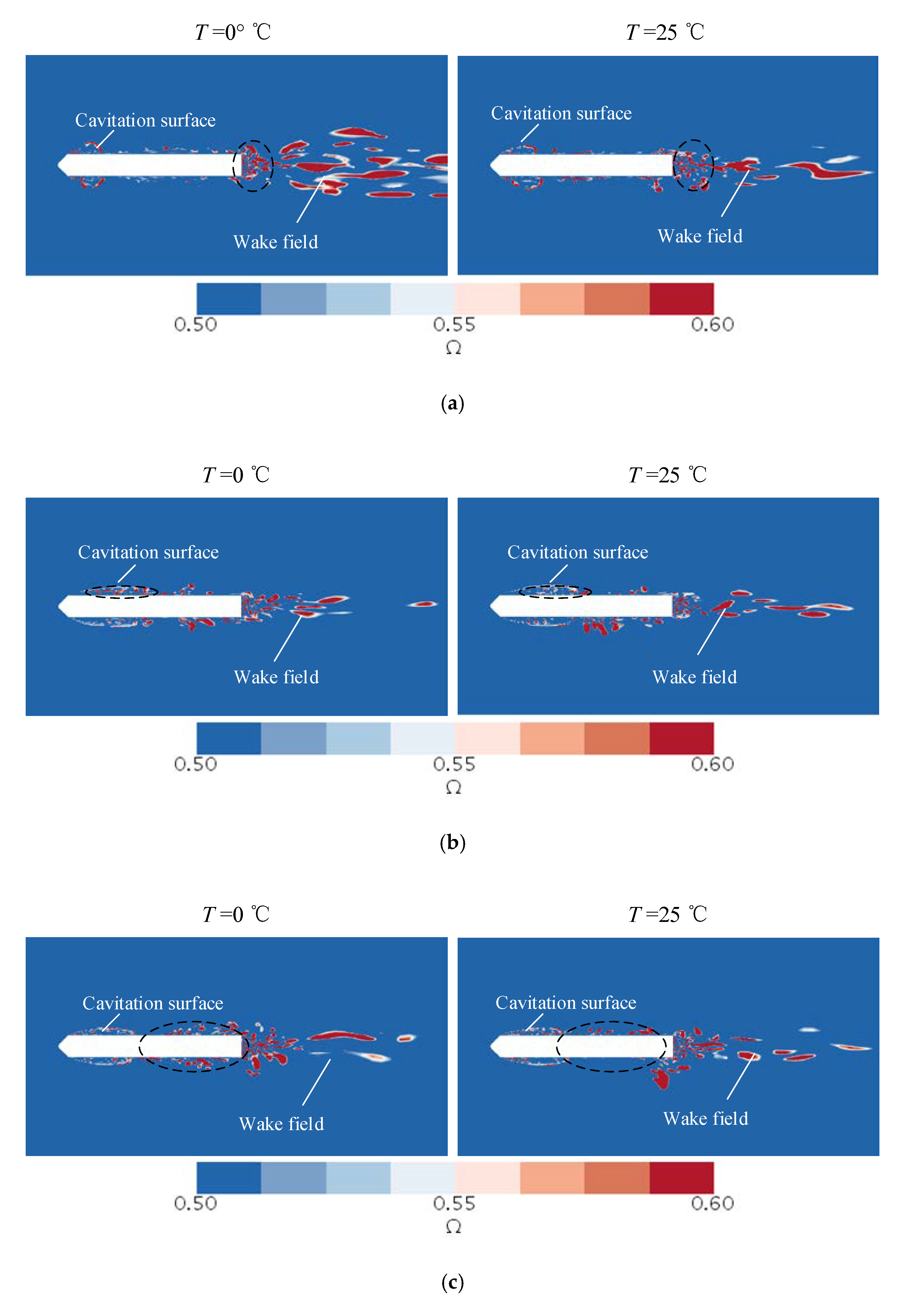
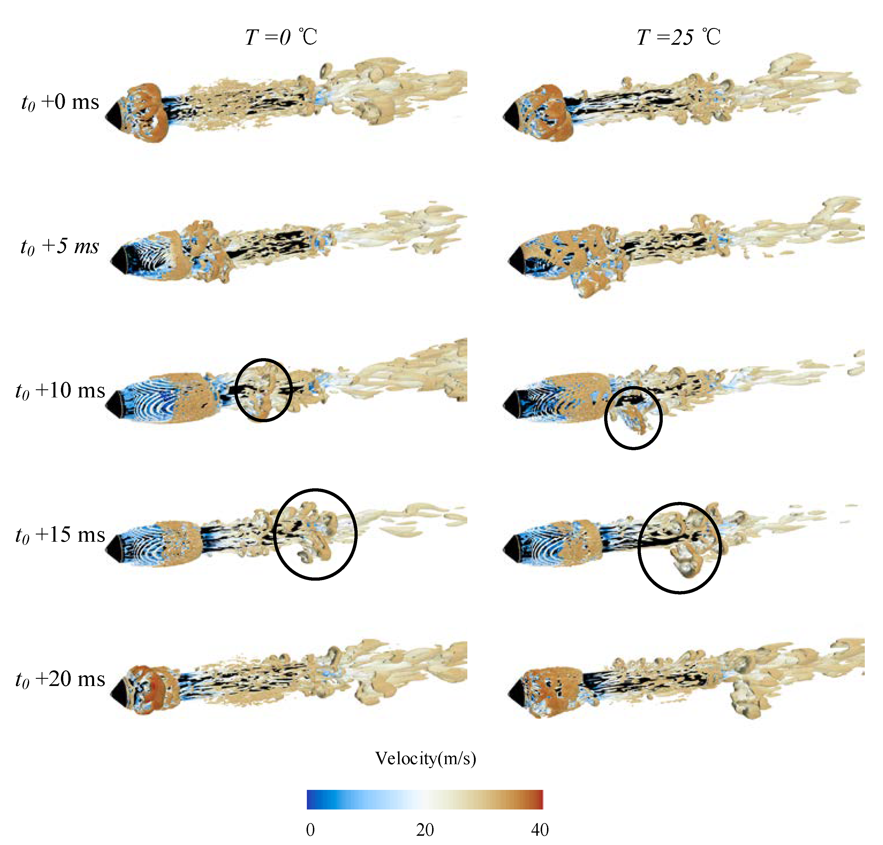
The temperature changes the vortex structure. At lower temperatures, during the cavity development stage, a larger number of linear vortex structures appear in the model wake area, and the vortex structure is significantly stronger than under higher-temperature conditions. In the cavity stabilization stage, a lower temperature enlarges the vortex structure inside the cavity, thus accelerating the shedding of the cavity and shortening the cavity shedding cycle. Finally, in the cavity shedding stage, lower temperatures enhance the model wall vortex structure. In general, we found that the wake field vortex structure changes more drastically at the lower temperature.

(3)

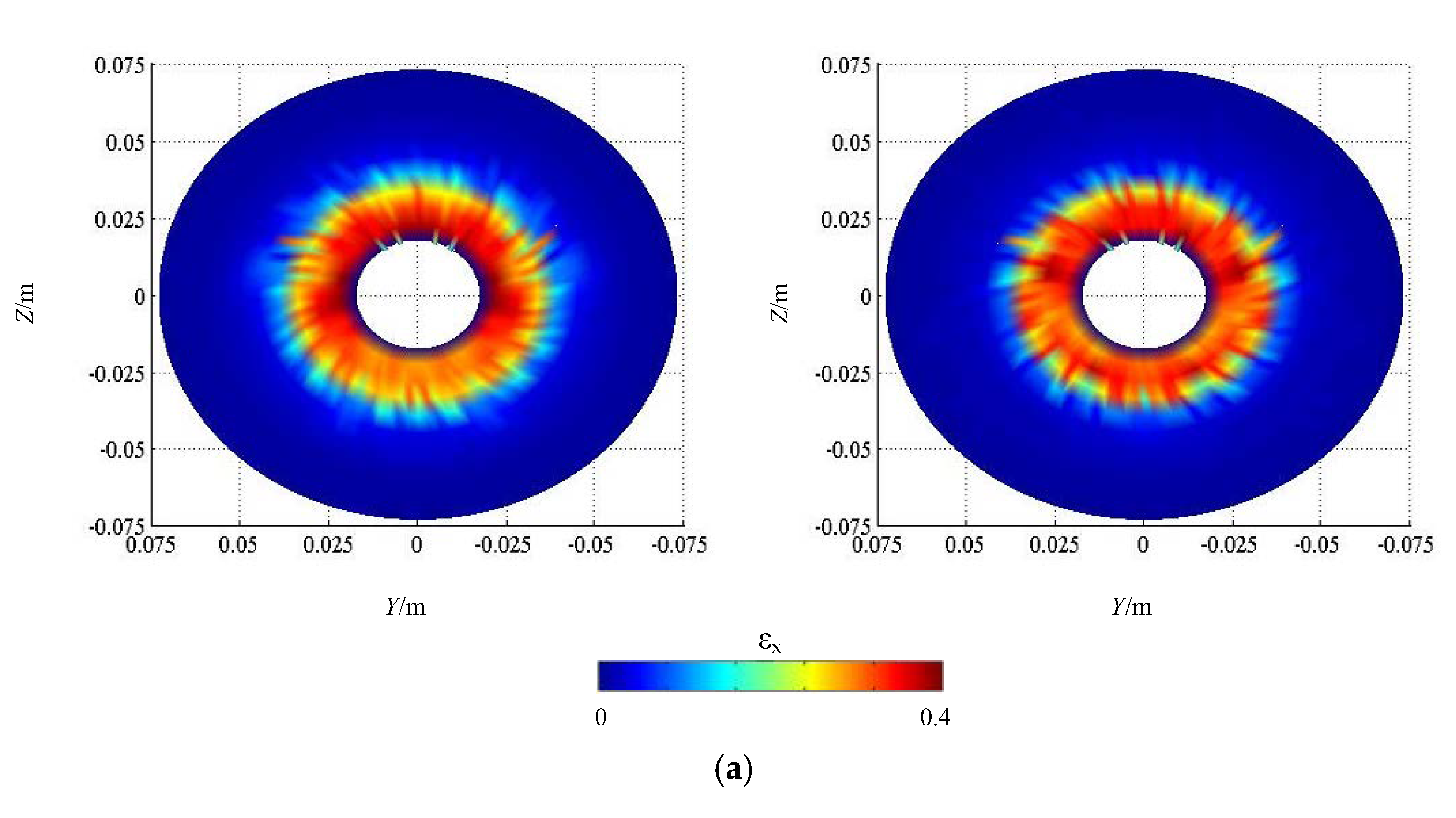
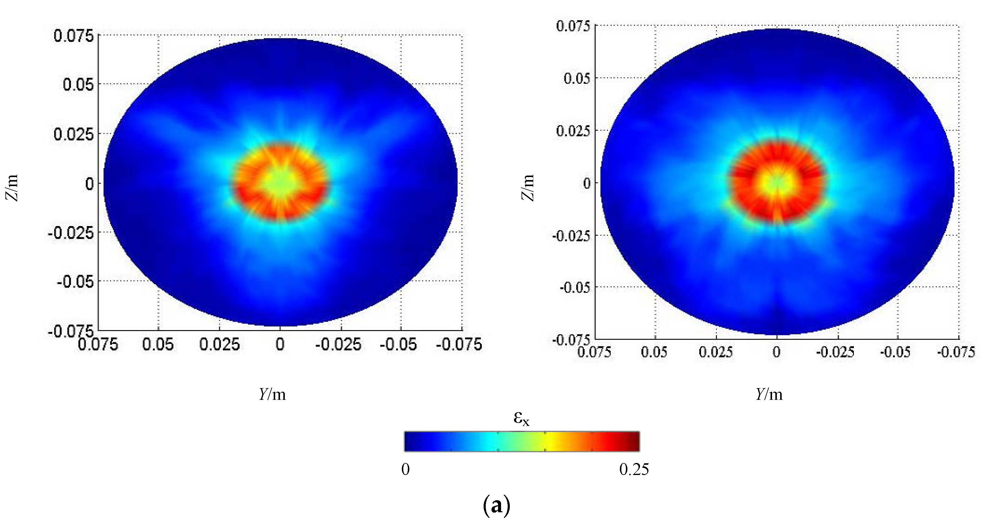
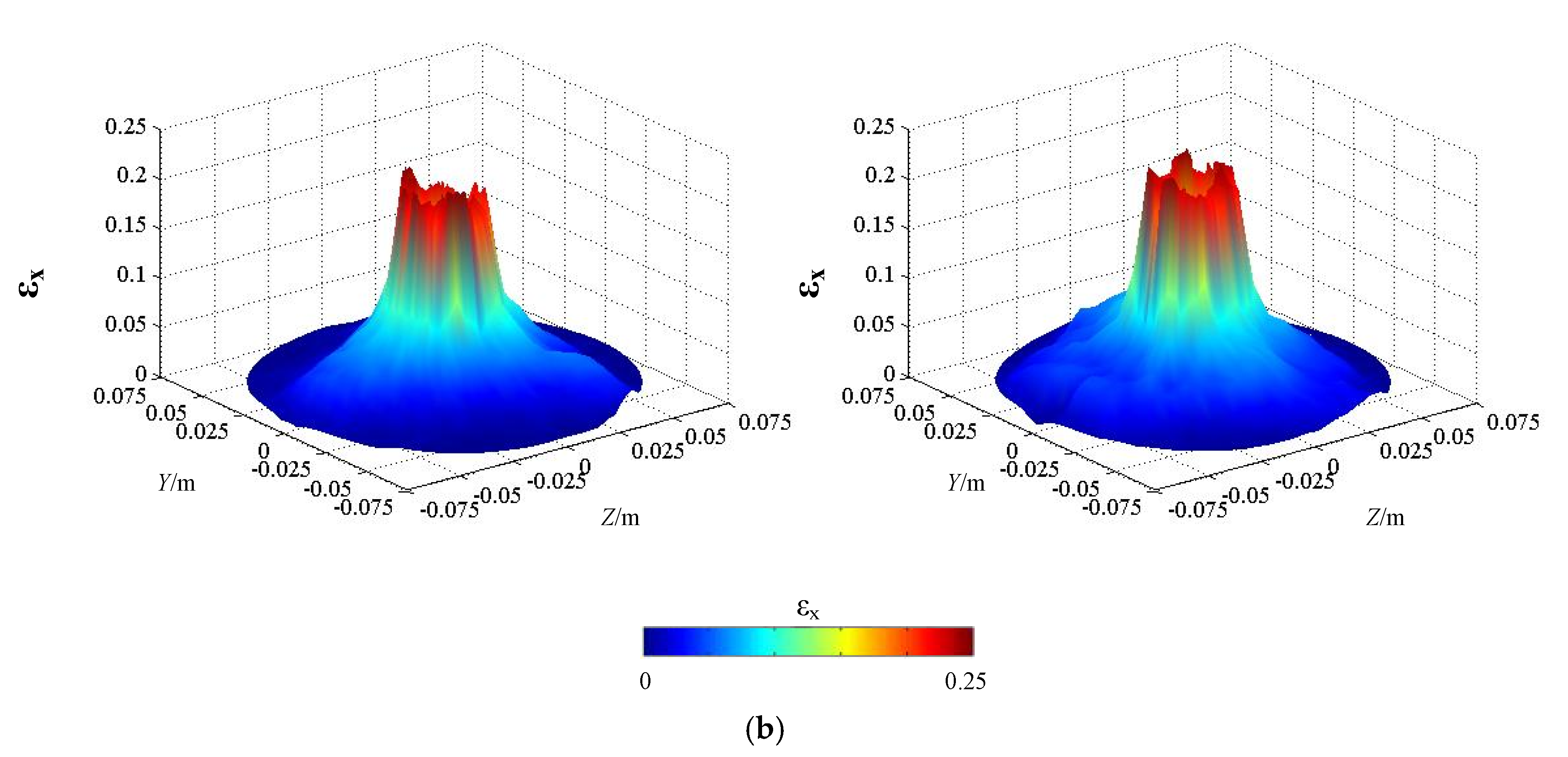
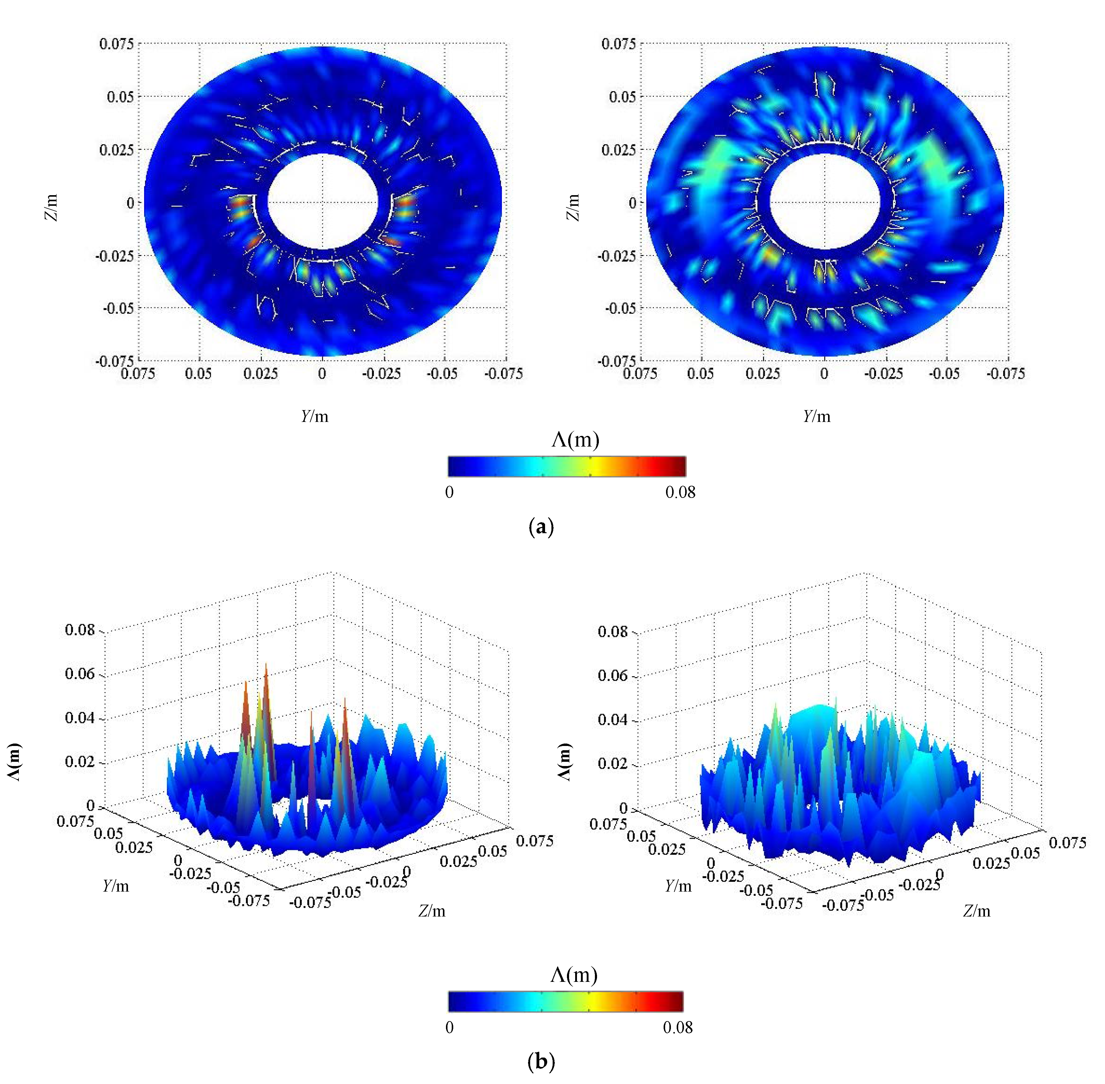
The temperature affects the velocity pulsations around the model. At lower temperatures, the velocity pulsations are reduced, and this has a more significant impact on the wake flow field than the flow field inside the cavity. The lower temperature increases the turbulence dissipation rate and reduces the overall turbulence. At the same time, lower temperatures reduce the turbulence integral scale both outside and inside the cavity. The influence on the tail flow field is mainly concentrated on the two sides of the model tail, that is, the cavity moves downstream, and large-scale shedding becomes small-scale shedding.

In this paper, through numerical simulation of the axisymmetric body, the flow structure characteristics of the cavitation flow field are obtained. The focus is on the influence of temperature on the temporal and spatial distribution of natural cavitation flow.

Based on the axisymmetric body that is simulated, obtaining structural characteristics of flow cavitation flow field focuses on the effect of temperature on the spatial and temporal distribution of the natural air stream.

Although some research progress has been made, the modeling process of cavitation multiphase flow is still slightly inadequate. The sensitivity of grid independence is not compared, and the dependence of the number of generations at different time steps is not considered enough. Although some research progress has been made, the modeling process of cavitation multiphase flow is still slightly inadequate. The sensitivity of grid independence is not compared, and the dependence of the number of generations at different time steps is not considered enough.

Although research has made some progress, there are still some shortcomings in the process of multiphase flow modeling, there is no comparison for grid-independent sensitivity, and research is still lacking on the number of different time steps in generation-dependent considerations.

In the follow-up research process, the grid sensitivity and the number of iterations will be analyzed more deeply.

References

1. Batchelor, C.K.; Batchelor, G.K. An Introduction to Fluid Dynamics; Cambridge University Press: Cambridge, UK, 2000. [Google Scholar]
2. Peng, C.; Tian, S.; Li, G.; Sukop, M.C. Simulation of multiple cavitation bubbles interaction with single-component multiphase Lattice Boltzmann method. Int. J. Heat Mass Transf. 2019, 137, 301–317. [Google Scholar] [CrossRef]
3. Sun, T.-Z.; Zong, Z.; Zou, L.; Wei, Y.; Jiang, Y. Numerical investigation of unsteady sheet/cloud cavitation over a hydrofoil in thermo-sensitive fluid. J. Hydrodyn. 2017, 29, 987–999. [Google Scholar] [CrossRef]
4. Wang, Y.; Xu, C.; Wu, X.; Huang, C.; Wu, X. Ventilated cloud cavitating flow around a blunt body close to the free surface. Phys. Rev. Fluids 2017, 2, 084303. [Google Scholar] [CrossRef]
5. Pendar, M.-R.; Roohi, E. Cavitation characteristics around a sphere: An LES investigation. Int. J. Multiph. Flow 2018, 98, 1–23. [Google Scholar] [CrossRef]
6. Liu, M.; Tan, L.; Cao, S. Cavitation–Vortex–Turbulence Interaction and One-Dimensional Model Prediction of Pressure for Hydrofoil ALE15 by Large Eddy Simulation. J. Fluids Eng. 2018, 141, 021103. [Google Scholar] [CrossRef]
7. Sun, T.; Xie, Q.; Zou, L.; Wang, H.; Xu, C. Numerical investigation of unsteady cavitation dynamics over a naca66 hydrofoil near a free surface. J. Mar. Sci. Eng. 2020, 8, 341. [Google Scholar] [CrossRef]
8. Yang, D.; Xiong, Y.; Guo, X. Drag reduction of a rapid vehicle in supercavitating flow. Int. J. Nav. Arch. Ocean Eng. 2017, 9, 35–44. [Google Scholar] [CrossRef] [Green Version]
9. Akbari, M.A.; Mohammadi, J.; Fereidooni, J. A dynamic study of the high-speed oblique water entry of a stepped cylindrical-cone projectile. J. Braz. Soc. Mech. Sci. Eng. 2021, 43, 1–15. [Google Scholar] [CrossRef]
10. Huang, B.; Qiu, S.-C.; Li, X.-B.; Wu, Q.; Wang, G.-Y. A review of transient flow structure and unsteady mechanism of cavitating flow. J. Hydrodyn. 2019, 31, 429–444. [Google Scholar] [CrossRef]
11. Knapp, R.T. Recent investigations of the mechanics of cavitation and cavitation damage. Wear 1958, 1, 455. [Google Scholar] [CrossRef]
12. Reisman, G.E.; Wang, Y.-C.; Brennen, C.E. Observations of shock waves in cloud cavitation. J. Fluid Mech. 1998, 355, 255–283. [Google Scholar] [CrossRef] [Green Version]
13. Passandideh-Fard, M.; Roohi, E. Transient simulations of cavitating flows using a modified volume-of-fluid (VOF) technique. Int. J. Comput. Fluid Dyn. 2008, 22, 97–114. [Google Scholar] [CrossRef]
14. Ganesh, H.; Mäkiharju, S.A.; Ceccio, S.L. Bubbly shock propagation as a mechanism for sheet-to-cloud transition of partial cavities. J. Fluid Mech. 2016, 802, 37–78. [Google Scholar] [CrossRef] [Green Version]
15. Philipp, A.; Lauterborn, W. Cavitation erosion by single laser-produced bubbles. J. Fluid Mech. 1998, 361, 75–116. [Google Scholar] [CrossRef]
16. Arndt, R.E. Cavitation in vortical flows. Annu. Rev. Fluid Mech. 2002, 34, 143–175. [Google Scholar] [CrossRef]
17. Yuan, C.; Song, J.; Zhu, L.; Liu, M. Numerical investigation on cavitating jet inside a poppet valve with special emphasis on cavitation-vortex interaction. Int. J. Heat Mass Transf. 2019, 141, 1009–1024. [Google Scholar] [CrossRef]
18. Wang, C.-C.; Huang, B.; Wang, G.-Y.; Duan, Z.-P.; Ji, B. Numerical simulation of transient turbulent cavitating flows with special emphasis on shock wave dynamics considering the water/vapor compressibility. J. Hydrodyn. 2018, 30, 573–591. [Google Scholar] [CrossRef]
19. Ji, B.; Ji, B.; Arndt, R.E.; Wu, Y. Numerical simulation of three dimensional cavitation shedding dynamics with special emphasis on cavitation–vortex interaction. Ocean Eng. 2014, 87, 64–77. [Google Scholar] [CrossRef]
20. De Giorgi, M.G.; Fontanarosa, D.; Ficarella, A. Characterization of unsteady cavitating flow regimes around a hydrofoil, based on an extended schnerr–sauer model coupled with a nucleation model—sciencedirect. Int. J. Multiph. Flow 2019, 115, 158–180. [Google Scholar] [CrossRef]
21. Kadivar, E.; Timoshevskiy, M.V.; Pervunin, K.S.; El Moctar, O. Experimental and numerical study of the cavitation surge passive control around a semi-circular leading-edge flat plate. J. Mar. Sci. Technol. 2020, 25, 1010–1023. [Google Scholar] [CrossRef]
22. Timoshevskiy, M.V.; Ilyushin, B.B.; Pervunin, K.S. Statistical structure of the velocity field in cavitating flow around a 2D hydrofoil. Int. J. Heat Fluid Flow 2020, 85, 108646. [Google Scholar] [CrossRef]
23. Sun, T.; Ma, X.; Wei, Y.; Wang, C. Computational modeling of cavitating flows in liquid nitrogen by an extended transport-based cavitation model. Sci. China Ser. E: Technol. Sci. 2016, 59, 337–346. [Google Scholar] [CrossRef]
24. Chen, T.; Huang, B.; Wang, G.-Y.; Zhao, X. Numerical study of cavitating flows in a wide range of water temperatures with special emphasis on two typical cavitation dynamics. Int. J. Heat Mass Transf. 2016, 101, 886–900. [Google Scholar] [CrossRef]
25. Holl, J.W.; Billet, M.L.; Weir, D.S. Thermodynamic effects on developed cavitation. J. Fluids Eng. 1975, 97, 507. [Google Scholar] [CrossRef]
26. Cervone, A.; Bramanti, C.; Rapposelli, E.; D’Agostino, L. Thermal Cavitation Experiments on a NACA 0015 Hydrofoil. J. Fluids Eng. 2005, 128, 326–331. [Google Scholar] [CrossRef]
27. Franc, J.-P.; Rebattet, C.; Coulon, A. An Experimental Investigation of Thermal Effects in a Cavitating Inducer. J. Fluids Eng. 2004, 126, 716–723. [Google Scholar] [CrossRef]
28. Petkovšek, M.; Dular, M. Experimental study of the thermodynamic effect in a cavitating flow on a simple Venturi geometry. J. Phys. Conf. Ser. 2015, 656, 012179. [Google Scholar] [CrossRef] [Green Version]
29. Chen, T.; Huang, B.; Wang, G.; Zhang, H.; Wang, Y. Numerical investigation of thermo-sensitive cavitating flows in a wide range of free-stream temperatures and velocities in fluoroketone. Int. J. Heat Mass Transf. 2017, 112, 125–136. [Google Scholar] [CrossRef]
30. Sun, T.; Wei, Y.; Zou, L.; Jiang, Y.; Xu, C.; Zong, Z. Numerical investigation on the unsteady cavitation shedding dynamics over a hydrofoil in thermo-sensitive fluid. Int. J. Multiph. Flow 2019, 111, 82–100. [Google Scholar] [CrossRef]
31. Wang, C.; Wang, G.; Huang, B. Characteristics and dynamics of compressible cavitating flows with special emphasis on com-pressibility effects. Int. J. Multiph. Flow 2020, 130, 103357. [Google Scholar] [CrossRef]
32. Coutier-Delgosha, O.; Reboud, J.L.; Delannoy, Y. Numerical simulation of the unsteady behaviour of cavitating flows. Int. J. Numer. Methods Fluids. 2003, 42, 527–548. [Google Scholar]
33. Wu, J.; Wang, G.; Shyy, W. Time-dependent turbulent cavitating flow computations with interfacial transport and filter-based models. Int. J. Numer. Methods Fluids 2005, 49, 739–761. [Google Scholar] [CrossRef]
34. Zahiri, A.P.; Roohi, E. Anisotropic minimum-dissipation (amd) subgrid-scale model implemented in openfoam: Verification and assessment in single-phase and multi-phase flows. Comput Fluids 2018, 180, 190–205. [Google Scholar] [CrossRef]
35. Chen, Y.; Li, J.; Gong, Z.; Chen, X.; Lu, C. Large eddy simulation and investigation on the laminar-turbulent transition and turbulence-cavitation interaction in the cavitating flow around hydrofoil. Int. J. Multiph. Flow 2019, 112, 300–322. [Google Scholar] [CrossRef]
36. An, H.; Sun, P.; Ren, H.; Hu, Z. CFD-based numerical study on the ventilated supercavitating flow of the surface vehicle. Ocean Eng. 2020, 214, 107726. [Google Scholar] [CrossRef]
37. Huang, B.; Young, Y.L.; Wang, G.; Shyy, W.; Huang, B. Combined Experimental and Computational Investigation of Unsteady Structure of Sheet/Cloud Cavitation. J. Fluids Eng. 2013, 135, 071301. [Google Scholar] [CrossRef]
38. Long, X.; Cheng, H.; Ji, B.; Arndt, R.E.; Peng, X. Large eddy simulation and Euler–Lagrangian coupling investigation of the transient cavitating turbulent flow around a twisted hydrofoil. Int. J. Multiph. Flow 2018, 100, 41–56. [Google Scholar] [CrossRef]
39. Sun, T.; Zhang, X.; Xu, C.; Zhang, G.; Wang, C.; Zong, Z. Experimental investigation on the cavity evolution and dynamics with special emphasis on the development stage of ventilated partial cavitating flow. Ocean Eng. 2019, 187, 106140. [Google Scholar] [CrossRef]
40. Sun, T.; Wang, Z.; Zou, L.; Wang, H. Numerical investigation of positive effects of ventilated cavitation around a NACA66 hydrofoil. Ocean Eng. 2020, 197, 106831. [Google Scholar] [CrossRef]
41. Huang, R.-F.; Du, T.-Z.; Wang, Y.-W.; Huang, C.-G. Numerical investigations of the transient cavitating vortical flow structures over a flexible NACA66 hydrofoil. J. Hydrodyn. 2020, 32, 865–878. [Google Scholar] [CrossRef]
42. Ji, B.; Luo, X.; Arndt, R.E.; Peng, X.; Wu, Y. Large Eddy Simulation and theoretical investigations of the transient cavitating vortical flow structure around a NACA66 hydrofoil. Int. J. Multiph. Flow 2015, 68, 121–134. [Google Scholar] [CrossRef] [Green Version]
43. Lidtke, A.K.; Humphrey, V.F.; Turnock, S.R. Feasibility study into a computational approach for marine propeller noise and cavitation modelling. Ocean Eng. 2016, 120, 152–159. [Google Scholar] [CrossRef] [Green Version]
44. Kunz, R.F.; Lindau, J.W.; Kaday, T.A. Unsteady RANS and detached eddy simulations of cavitating flow over a hydrofoil. In Proceedings of the Fifth International Symposium on Cavitation, Osaka, Japan, 1–4 November 2003. [Google Scholar]
45. Girimaji, S.S. Partially-Averaged Navier-Stokes Model for Turbulence: A Reynolds-Averaged Navier-Stokes to Direct Numerical Simulation Bridging Method. J. Appl. Mech. 2006, 73, 413–421. [Google Scholar] [CrossRef]
46. Gao, G.H.; Zhao, J.; Ma, F.; Luo, W.D. Hybrid RANS–LES Modeling for Unsteady Cavitating Flow Simulation. Appl. Mech. Mater. 2012, 152, 1187–1190. [Google Scholar] [CrossRef]
47. Usta, O.; Korkut, E.A. study for cavitating flow analysis using DES model. Ocean Eng. 2018, 160, 397–411. [Google Scholar] [CrossRef]
48. Spalart, P.R. Comments on the feasibility of LES for wings, and on a hybrid RANS/LES approach. In Proceedings of First AFOSR International Conference on DNS/LES; Greyden Press: Dayton, OH, USA, 1997. [Google Scholar]
49. Menter, F.R.; Kuntz, M.; Langtry, R. Ten years of industrial experience with the SST turbulence model. Turbulence Heat Mass Transf. 2003, 4, 625–632. [Google Scholar]
50. Rayleigh, L. VIII. On the pressure developed in a liquid during the collapse of a spherical cavity. Lond. Edinb. Dublin Philos. Mag. J. Sci. 1917, 34, 94–98. [Google Scholar] [CrossRef]
51. Plesset, M.S. The Dynamics of Cavitation Bubbles. J. Appl. Mech. 1949, 16, 277–282. [Google Scholar] [CrossRef]
52. Schnerr, G.H.; Sauer, J. Physical and numerical modeling of unsteady cavitation dynamics. In Proceedings of the Fourth International Conference on Multiphase Flow, New Orleans, LA, USA, 27 May–1 June 2001. [Google Scholar]
53. Brennen, C.E. Cavitation and Bubble Dynamics; Cambridge University Press (CUP): New York, NY, USA, 2014. [Google Scholar]
54. Zhang, X.; Wang, C.; Wei, Y.; Sun, T. Experimental investigation of unsteady characteristics of ventilated cavitation flow around an under-water vehicle. Adv. Mech. Eng. 2016, 8. [Google Scholar] [CrossRef] [Green Version]
55. Liu, C.; Wang, Y.; Yang, Y.; Duan, Z. New omega vortex identification method. Sci. China Ser. G: Physics, Mech. Astron. 2016, 59, 1–9. [Google Scholar] [CrossRef]
56. Piomelli, U.; Balint, J.-L.; Wallace, J.M. On the validity of Taylor’s hypothesis for wall-bounded flows. Phys. Fluids A: Fluid Dyn. 1989, 1, 609–611. [Google Scholar] [CrossRef]
Figure 1. Experimental setup and computational geometric model.
Jmse 09 00024 g001
Figure 2. Experimental setup and computational geometric model.
Jmse 09 00024 g002
Figure 3. (a) Position of the monitoring surface in the two-dimensional calculation domain; (b) rear view of the monitoring surface.
Jmse 09 00024 g003
Figure 4. Mesh generation around the model.
Jmse 09 00024 g004
Figure 5. Comparison of natural cavity evolution: (a) experimental observation; (b) numerical simulation; (c) prediction of XOY surface water volume fraction. (The value of water volume fraction is 0–1.)
Jmse 09 00024 g005
Figure 6. Comparison of pressure fluctuations on the surface of the model at P2 (a) and P4 (b).
Jmse 09 00024 g006
Figure 7. Comparison of natural cavity evolution between 0 °C and 25 °C cases.
Jmse 09 00024 g007
Figure 8. Comparison of the natural cavity volume change between 0 °C and 25 °C cases.
Jmse 09 00024 g008
Figure 9. Comparison of natural cavitation pressure pulsation at points P1 (a) and P3 (b) at two temperatures.
Jmse 09 00024 g009
Figure 10. Comparison of power spectral density (PSD) corresponding to natural cavitation pressure pulsation at points P1 (a) and P3 (b) at two temperatures.
Jmse 09 00024 g010
Figure 11. Comparison of two-dimensional natural cavitation vortex structure based on Ω method at 0 °C and 25 °C. (a) Comparison of two-dimensional vortex structures during cavity development. (b) Comparison of two-dimensional vortex structures during cavity stabilization. (c) Comparison of two-dimensional vortex structures during cavity shedding.
Jmse 09 00024 g011
Figure 12. Comparison of the vortex structure of natural cavitation at 0 °C and 25 °C (isosurface of Ω = 0.52 colored according to velocity magnitude).
Jmse 09 00024 g012
Figure 13. Comparison of turbulence intensity inside the cavity. (a) Two-dimensional turbulence intensity inside the cavity at 0 °C (left) and 25 °C (right). (b) Three-dimensional turbulence intensity inside the cavity at 0 °C (left) and 25 °C (right).
Jmse 09 00024 g013aJmse 09 00024 g013b
Figure 14. Comparison of turbulence intensity of wake field. (a) Two-dimensional turbulence in intensity of wake field at 0 °C (left) and 25 °C (right). (b) Three-dimensional turbulence intensity of wake field at 0 °C (left) and 25 °C (right).
Jmse 09 00024 g014aJmse 09 00024 g014b
Figure 15. Comparison of turbulence integral scales inside the cavity. (a) Two-dimensional turbulence integral scale inside the cavity at 0 °C (left) and 25 °C (right). (b) Three-dimensional turbulence integral scale inside the cavity at 0 °C (left) and 25 °C (right).
Jmse 09 00024 g015
Figure 16. Comparison of turbulence integral scales of the wake field. (a) Two-dimensional turbulence integral scale of the wake field at 0 °C (left) and 25 °C (right). (b) Three-dimensional turbulence integral scale of the wake field at 0 °C (left) and 25 °C (right).
Jmse 09 00024 g016
Publisher’s Note: MDPI stays neutral with regard to jurisdictional claims in published maps and institutional affiliations.