Abstract
Oil spill accidents have seriously harmed the marine environment. Effective oil spill monitoring can provide strong scientific and technological support for emergency response of law enforcement departments. Shipborne radar can be used to monitor oil spills immediately after the accident. In this paper, the original shipborne radar image collected by the teaching-practice ship Yukun of Dalian Maritime University during the oil spill accident of Dalian on 16 July 2010 was taken as the research data, and an oil spill detection method was proposed by using LBP texture feature and K-means algorithm. First, Laplacian operator, Otsu algorithm, and mean filter were used to suppress the co-frequency interference noises and high brightness pixels. Then the gray intensity correction matrix was used to reduce image nonuniformity. Next, using LBP texture feature and K-means clustering algorithm, the effective oil spill regions were extracted. Finally, the adaptive threshold was applied to identify the oil films. This method can automatically detect oil spills in shipborne radar image. It can provide a guarantee for real-time monitoring of oil spill accidents.
1. Introduction
With the rapid development of offshore industries of oil exploitation and transportation, oil spill accidents occurred frequently [1,2]. Oil spills are very harmful to the marine environment [3,4,5]. It is of great significance to carry out oil spill monitoring and early warning quickly and effectively. At present, there are five deployment modes of remote sensing sensors in oil spill monitoring and early warning, which are space-based, air-based, shore-based, ship-based, and platform-based [6,7]. Satellite sensors are widely used to detect oil films in large-area [8]. Due to the periodicity of satellite data acquisition, they are impossible to monitor oil spills in real-time. With the rapid development of unmanned aerial vehicle (UAV) technology, the oil spill monitoring technology of airborne sensors have boomed [9]. However, the UAV monitoring manners are still restricted by the weather and sea states, often unable to carry out the missions. Shipborne radar can be installed on shores, ships, and platforms. It can execute large-scale oil spill monitoring and early warning missions under severe weather. It is one of the most effective sensors that can arrive at the site at once after the oil spill accident for cooperation with the emergency command and the clean-up action, which has broad application value and promotion prospect.
In shipborne radar images with sea clutter information, oil films show relatively dark image features compared to the surroundings. These features can be used to extract the oil films. The development of oil spill monitoring and early warning technology of shipborne radar is still in its infancy. In 1988, Tennyson proved the possibility of the shipborne radar oil spill detection under the appropriate sea states [10]. After that, he attempted to extract the oil spill information from the shipborne radar image by selectively intercepting the sea clutter image [11]. In 1991, Atanassov et al. verified the feasibility of using shipborne radar to identify the size, shape, and dynamic information of oil spills based on statistical analysis [12]. Since then, there have been commercial products used for oil spill monitoring and early warning, such as Sigma of Rutter company [13,14,15]. However, due to the confidentiality policy of commercial companies, the core technologies have not yet been published. Since 2010, based on the shipboard radar images collected in the oil spill accident of Dalian on July 16, 2010, the researchers of Dalian Maritime University have successively published the achievements of oil spill monitoring by using adaptive threshold methods, active contour models, and machine learning methods [16,17,18,19,20,21,22,23].
Machine learning has been successfully applied in image pattern recognition, and it has also been well verified in oil film identification of spaceborne and airborne images. Cao et al. developed an oil spill automatic classification system through active learning (AL) based on a relatively small number of samples. They extracted oil spill points from 198 RadarSat images covering the east and west coasts of Canada from 2004 to 2013 [24]. In 2014, based on the adaptive Weibull multiplicative model and multi-layer perceptron (MLP) neural network, Alireza and Natascha carried out automatic oil spill detection and classification for the images of ENVISAT and the second European Space Agency satellite [25]. Liu et al. realized the automatic classification of oil films in airborne visible infrared imaging spectrometer (AVIRIS) hyperspectral images based on the classification model of spectral indexes-based band selection and convolution neural network [26]. Based on layered unsupervised training, Chen et al. used machine learning methods such as layered self-coding and deep belief network to classify the oil spills from RadarSat-2 SAR images acquired during the oil spill prevention and control exercise of Norwegian in 2011 [27]. Xu et al. classified oil spills based on artificial neural network (ANN), generalized additive model (GAM), penalty linear discriminant Analysis (PLDA), and other machine learning classifiers in the RadarSat-1 images of eastern and western coasts of Canada from 2004 to 2008 [28]. Chen and Lu identify the oil films from the images of the optical camera on a UAV using subcategory perceptual feature selection and SVM classifier [29].
Because of the relatively dark characteristics of the oil spills compared to sea waves in the shipborne radar images, the automatic segmentation of the oil films is difficult. Machine learning used in oil film identification of shipborne radar image is infrequent. An oil spill detection method was proposed by using machine learning method in this paper. After image preprocessing, LBP texture feature and K-means clustering algorithm were used to extract the oil spill effective monitoring regions. Then, the adaptive threshold was applied to recognize the oil films. This method can be completed automatically and has a certain promotional value.
2. Materials and Methods
2.1. Original Shipborne Radar Image
On 16 July 2010, an oil pipeline exploded in Dalian (Figure 1), China. At least 1500 tons of crude oil spilled into the sea, seriously harming the ecological environment, tourism, and fishery. Operations of emergency rescue and decontamination continued for a long time.
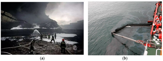
Figure 1.
The oil spill accident of Dalian on 16 July 2010; (a) emergency rescue; (b) physical recovery of oil spill.
The experimental image was collected by the teaching-practice ship Yukun (Figure 2) of Dalian Maritime University during the cruise mission on 21 July 2010, as shown in Figure 3. The size of the image is 1024 × 1024 pixels. The acquisition time is 23:19:58. The detection range is 0.75 nautical miles (NM). The parameters of radar hardware are shown in Table 1. The experimental software platform is Matlab.
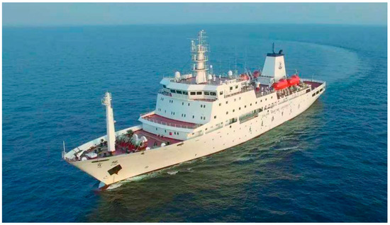
Figure 2.
The teaching-practice ship Yukun of Dalian Maritime University.
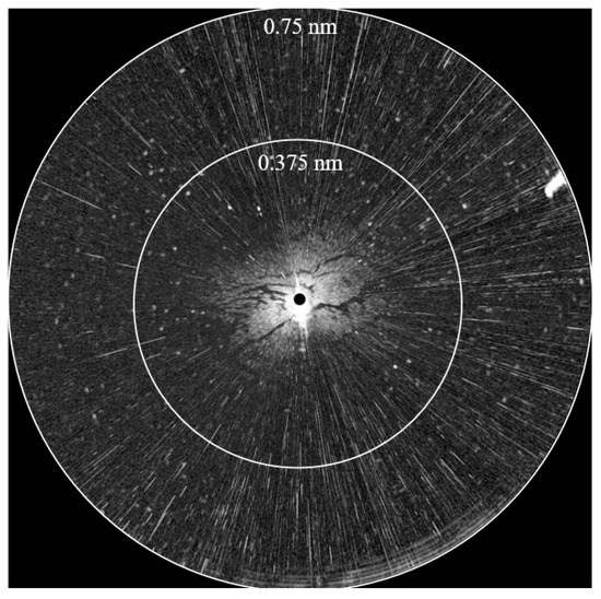
Figure 3.
Original shipborne radar image in the polar coordinate system.

Table 1.
Parameters of shipborne radar.
2.2. Experimental Procedures
The experimental flow is shown in Figure 4. The original shipborne radar image was converted from the polar coordinate system (the position is described with distance and azimuth) to the Cartesian coordinate system (the horizontal axis is in angle and the vertical axis is in meter). Then, Laplace operator and Otsu algorithm were used to extract the co-frequency interferences and highlight pixels. And mean filter was used to suppress them. Next, the gray intensity correction matrix (GICM) was used to reduce image nonuniformity. After that, the local contrast of the image was enhanced to obtain the preprocessed image. Then, LBP texture feature and K-means clustering algorithm were applied to extract the effective oil spill region. And the local adaptive threshold was used to segment the oil films. Finally, the result was converted to the polar coordinate system.
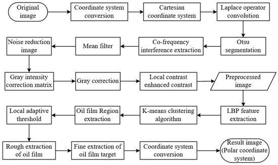
Figure 4.
Experimental procedures.
2.3. Methods of Data Preprocessing
2.3.1. Coordinate System Transformation
The original shipborne radar image was acquired in the Cartesian coordinate system, as shown in Figure 5. This image was difficult for non-professionals to understand. For real application, it was transformed into a polar coordinate system (Figure 3). However, there were many image features that were prominent in the Cartesian coordinate system. For example, in the Cartesian coordinate system, the co-frequency interferences were only the highlight rays in the vertical axis direction, as shown in Figure 6.
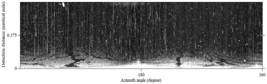
Figure 5.
Original shipborne radar image of the Cartesian coordinate system.
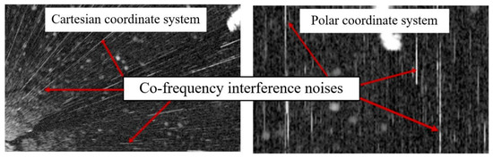
Figure 6.
Directional characteristics of co-frequency interference noises.
2.3.2. Laplace Operator
The Laplace operator was used to enhance the co-frequency interferences as follows:
where x and y are the abscissa and ordinate of the image, respectively.
2.3.3. Mean Filter
The mean filter was calculated to suppress the highlight pixel by two horizontal nearest non-noise pixels as:
where m is the number of horizontal noise pixels on the left side of the target pixel, n is the number of horizontal noise pixels on the right side.
2.3.4. GICM
Subtraction between the noise reduction image and its GICM can reduce image nonuniformity. The generation method of GICM used is as shown in Figure 7.
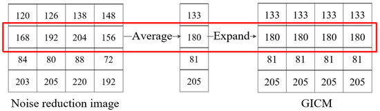
Figure 7.
Generation of gray intensity correction matrix (GICM) model.
2.3.5. CLAHE
The contrast limited adaptive histogram equalization (CLAHE) [30] model was used after the image gray level adjustment to increase the local contrast information of the oil film area. The implementation of CLAHE model is shown in Figure 8.
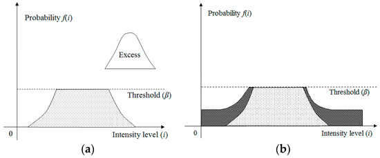
Figure 8.
The implementation of CLAHE model. (a) Values larger than threshold (β) are clipped off, and (b) excess is distributed to others.
2.4. Methods of Oil Film Segmentation
2.4.1. Local Binary Pattern
Texture is a kind of visual feature that reflects the same characteristics in the image. It is expressed by the gray distribution characteristics of the pixel and its s neighborhood, that is, local texture information. Therefore, the neighborhood window must be defined first. Ojala et al. proposed a local binary pattern (LBP) for texture feature extraction [31,32,33]. An LBP has the advantages of simple calculation and easy extraction. It is widely used for machine vision detection.
The gray image is divided into neighborhoods with the local window size (the size of the analysis region), such as 3 × 3 for LBP. The feature information of any pixel in the image is calculated from itself and its neighborhood. And the gray values of the center and its neighbors in each local window are compared. If the gray value of the neighbor is greater than the center pixel, it is marked as “1.” Otherwise, the neighbor is encoded by “0.” Then, the center value of this local window is replaced by the decimal LBP feature value for classification as Figure 9.
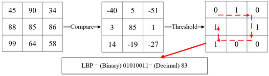
Figure 9.
Calculation method of LBP feature value.
LBP operator can be defined as:
where (x, y) denotes the center pixel of the neighborhood, i and ip denote the gray values of the center pixel and neighbors. n is the number of neighbors. s() denotes a symbolic function:
2.4.2. K-Means
MacQueen proposed the K-means unsupervised learning classification algorithm after summarizing the research of Cox, Fisher, and Sebestyen in 1967 [34,35,36,37]. K-means algorithm divides the data into K classes with minimum and maximum similarity within classes through iterations. The algorithm flow is as follows:
- K initial cluster centers ci (i = 1, 2, …, K) are selected randomly from the set S where S = {x1, x2, …, xn}.
- According to the similarity, the distance from each remaining instance to each cluster center is calculated and classified into the nearest cluster center category.
- The arithmetic mean of each cluster is recalculated as a new cluster center as:where |Si| is the total number of instances that are in cluster i.
- Judge the convergence of data clustering, if it tends to be stable, the clustering is over, otherwise continue to iterative calculation steps (b) and (c).
K-means algorithm is easy to implement and widely used in image segmentation [38,39,40], but it has some limitations. The final clustering will depend on the arbitrary selection of the cluster center and the size of K value. The random initial cluster center will lead to different clustering results and even lead to the clustering results falling into the local optimal value. In this paper, the K-means algorithm is used for image classification, the distance is the difference between their intensity levels.
2.4.3. Local Adaptive Threshold
Niblack proposed a local thresholding method for digital image segmentation [41] as:
where m is the local mean, s is the local standard deviation, and k is a user-defined parameter, which takes negative values. Sauvola modified the method to realize adaptive document image binarization [42] as:
where R is the dynamic range of standard deviation, and the parameter k gets positive values. Phansalskar [43] modified Sauvola method to deal with low contrast images as follows:
where p and q are constants. The value of q is above a particular value of the local mean, the exponential term becomes negligible. Phansalkar recommended k = 0.25, R = 0.5, p = 2, and q = 10. Because of the gray correction of the experimental data in the preprocessing stage, the image contrast is reduced. So, we use this method to segment the preprocessed image.
3. Results
3.1. Data Preprocessing
After Laplace operator convolution and Otsu segmentation of the shipborne radar image in Cartesian coordinate system, the highlighted pixels were extracted. The mean filter was used to suppress the highlighted pixels, as shown in Figure 10.
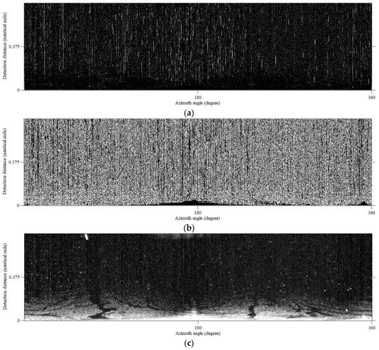
Figure 10.
Noise reduction image. (a) Convolution of Laplace operator, (b) Otsu method, and (c) mean filter.
Then, the GICM model of noise reduction image was used to adjust the gray distribution of the image as Figure 11a. The CLAHE algorithm was applied to enhance the local contrast of the oil film regions as Figure 11c. The oil films were more obvious in the color pattern image, as shown in Figure 11d.
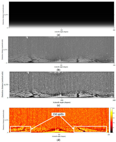
Figure 11.
Preprocessed result. (a) GICM of Figure 10d, (b) gray correction image, (c) enhancement the local contrast, and (d) oil spill regions in color pattern image.
3.2. Oil Spill Segmentation
Phansalskar’s local adaptive threshold was used to segment the preprocessed image (Figure 11c) as Figure 12. Because there were some false positive segmentation targets in the ship wake and regions with long distance. So, the effective oil spill regions were chosen at first.
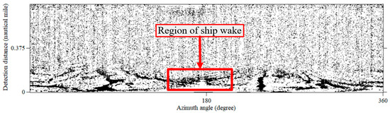
Figure 12.
Segmentation of local adaptive threshold.
LBP feature of preprocessed image (Figure 11c) was extracted as Figure 13a. The local window was 256 × 256 pixels. Then the image was divided into 3 classes (black, gray, and white) by K-means clustering method as Figure 13b. Keep the middle class as the oil spill regions and remove the regions far away and the ship’s wake in the image, as shown in Figure 13d.
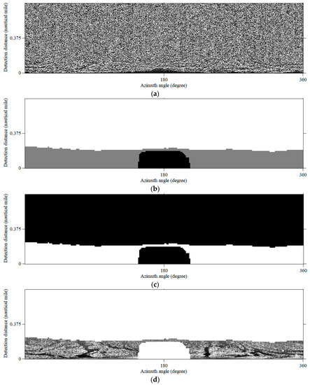
Figure 13.
Selection of oil spill region. (a) LBP feature extraction, (b) K-means clustering method, (c) middle class was remained as effective oil spill region, and (d) synthesis image.
Segmentation of local adaptive threshold was cropped by Figure 13c for rough extraction of oil films as Figure 14a. The image was reversed, and the speckles were removed to get precise oil film results as Figure 14b. Then oil film results and noise reduction image (Figure 10c) were synthesized as Figure 14c. Finally, the synthesis image was converted to a polar coordinate system.
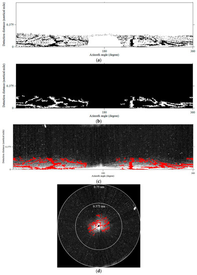
Figure 14.
Oil film detection results. (a) Rough extraction of oil films, (b) precise extraction of oil films, (c) oil film synthesis image, and (d) final result of polar coordinate system.
4. Discussion
4.1. Comparison of the Texture Features Applicability of LBP and GLCM
The gray level co-occurrence matrix (GLCM) and K-means clustering algorithm were also used to classify the texture features of the preprocessed image (Figure 11c), as shown in Figure 15. The computing time of our classification method was 11.6 s. It was extremely faster than the combination method of GLCM and K-means, which took 226.3 s. In addition, the pixels of middle-class extracted by GLCM and K-means method were not the effective regions for oil film identification, as shown in Figure 15b. If the top-class pixels were determined as the effective regions of oil films, the region of ship wake remained, and some oil spill regions might be lost, as shown in Figure 15c. Therefore, the LBP feature is more suitable for classifying the effective oil spill regions in the preprocessed image.
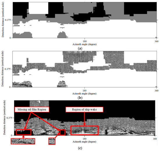
Figure 15.
Classification result of GLCM and K-means. (a) K-means clustering method of GLCM texture features, (b) middle-class information, and (c) top-class information.
4.2. Local Window Dimension Selection for Texture Feature Extraction
LBP window sizes of 64 × 64, 128 × 128, and 512 × 512 were used to extract the effective oil spill regions as Figure 16, and the compute time were shown in Table 2. Due to the computing process of the LBP texture feature, with the local window dimension enlarged, the running time increased. However, from the extraction of effective oil spill regions, the 256 × 256 window had the best effect between Figure 13d and Figure 16. Therefore, we recommend that the LBP window size here was 256 × 256. If the sea condition changes dramatically, such as abundant rain or high waves existed, the overall characteristics of the shipborne radar images will change greatly, and the size of the LBP window should be adjusted accordingly. It will increase the robustness of the proposed method that collecting adequate shipborne radar images with oil spill information in different sea conditions and establishing an adaptive parameter model. This is one of the priorities of future work.
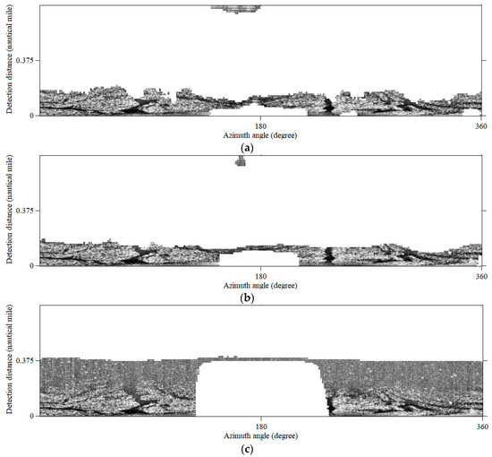
Figure 16.
The effective oil spill identification regions of different LBP window dimensions. (a) 64 × 64, (b) 128 × 128, and (c) 512 × 512.
Table 2.
Compute time of different LBP window dimensions.
4.3. Comparison between Local Adaptive Threshold and Single Threshold
Zhu et al. [16] proposed to extract oil films from the X-band shipborne radar image after gray-scale adjustment by Selecting a gray threshold manually (called Method 1 here). Method 1 was used to detect the oil spills of Figure 13d, and the gray threshold values were ”80,” “100,” and “120,” respectively, as shown in Figure 17. When the threshold setting was lower (‘80’), the entire oil films cannot be identified, as shown in Figure 17a. When the threshold setting was higher (120), a large number of error results appeared, as shown in Figure 17c. When the threshold was set to “100,” the result was fine and similar to our method, as shown in Figure 17b. However, false results were still obtained in areas without sea waves. Therefore, manual selection requires a lot of comparisons among results for the appropriate threshold. The local adaptive threshold can automatically extract the oil films from the shipborne radar image with better applicability.
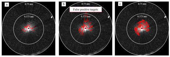
Figure 17.
Single threshold method. (a–c) are results of gray threshold of ‘80’, ‘100’ and ‘120’, respectively.
4.4. Comparison with Other Local Adaptive Thresholds
There are many methods of image adaptive threshold segmentation. For example, Bernsen proposes a threshold segmentation method for gray image [44]. The local Otsu (called Method 2 here) and Bernsen (called Method 3 here) methods are compared with the Phansalkar method here, and the segmentation results are shown in Figure 18a,b. Compared with Figure 12, Methods 2 and 3 used larger local thresholds, which results in more false-positive oil films Furthermore, the final results of both methods were also unideal as Figure 18c,d.
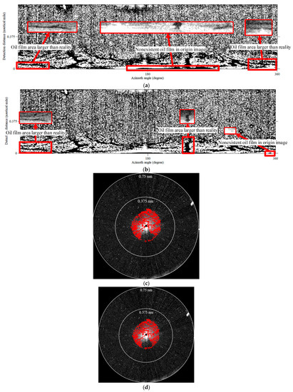
Figure 18.
Results of other local adaptive threshold methods. (a,b) are the rough segmentation of Methods 2 and 3, respectively. (c,d) are the final segmentation of Methods 2 and 3, respectively.
4.5. Comparison with Other Machine Learning Oil Spill Detection Method
Xu et al. [23] proposed an oil spill detection method of shipborne radar image based on SVM (called Method 4 here), as shown in Figure 19. Method 4 uses SVM method to classify ocean waves and then determines the effective monitoring range of oil spill according to gray gradient matrix. Due to the application of gray gradient matrix, the ship wake influence region cannot be eliminated as in Figure 19c. Therefore, it is necessary to eliminate the ship wake influence region in the result as Figure 19d. It means that Method 4 contains two effective oil spill region selection processes. Compared with their methods, we use LBP feature and K-means algorithm to select the effective area of oil film and eliminate the interference area of ship wake at the same time. In addition, when selecting the effective oil spill area, Method 4 needs to choose a suitable threshold through manual comparison. But our approach allows the whole process to be automated. Therefore, our method has obvious advantages in terms of efficiency and automatic calculation.
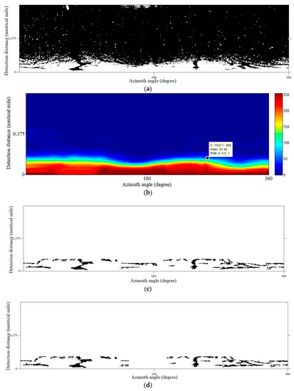
Figure 19.
Results of Method 4. (a) Classification of sea wave and background based on SVM; (b) Gray gradient matrix; (c) Preliminary extraction of oil film; (d) Final oil films.
4.6. Comparison with ACM
Active contour model (ACM) extracts the edge of the target by setting an initial contour and inverting it continuously. Xu et al. [22] proposed an improved LBF model [45] for oil film recognition of shipborne radar images (called Method 5 here). LBF model is a region-based ACM with a variable level set formulation. Starting with a pre-set contour C, a local window I(x): Ω → R of the image around y is divided into two regions of the target Rin and background Rout. The energy function is defined:
where λ1 and λ2 are previously defined. Cin and Cout are constants. f1(x) and f2(x) are fitting functions. K is a kernel function with the localization property of K(u) decreases and approaches zero as |u| increases. A Gaussian kernel was chosen as K(x) with a standard deviation of σ:
Due to the localization property of K(u), the contribution of I(x) to the LBF energy decreases to zero as y moves away from the central point x. Method 5 put forward dual-threshold method to eliminate the irregular spots segmented from LBF model as:
where A is the area of continuous pixels, Tin and Tout are the area thresholds of Rin and Rout, respectively. We use method 5 to extract the oil film target edges of Figure 13d, as shown in Figure 20. The window size of Gauss kernel was 9 × 9, σ = 2, λ1 = 1, λ2 = 2, i (iterations) = 20, Tin = 10, and Tout = 10.
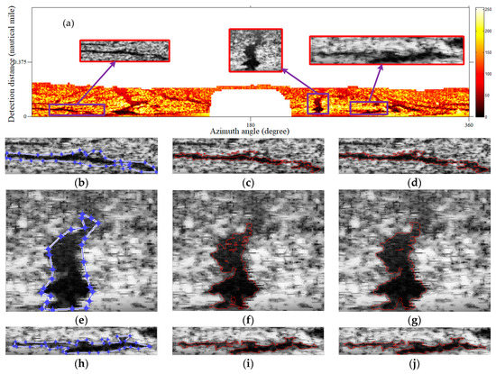
Figure 20.
Results of Method 5. (a) Image slice samples; (b,e,h) are the pre-set contours of tiles; (c,f,i) are the ACM results of 5 iterations; (d,g,j) are the ACM results of 20 iterations.
It took a long time to extract the oil film edges from the whole radar image using ACM. In addition, as the radar gray level becomes weaker from the near to the distant, and the gray distribution is also very uneven. Therefore, it is suggested here that the concerned oil films were extracted after slicing the image as in Figure 20a. From the segmentation results, when the number of iterations reaches 5, ACM can extract the rough edges of the targets. When the number of iterations reaches 20, the accurate edges of the concerned oil films can be obtained. Therefore, ACM is suitable for the extraction of specific oil films in the local window of shipborne radar gray image. It is worth mentioning that in the local window, the time consumed by 20 iterations of ACM is between 0.3 s and 0.4 s. So, the computational efficiency ACM is relatively high.
In general, ACM can accurately extract the oil film edge in the local window, but it was very difficult to extract all the oil films in the whole shipborne radar gray image at once. Our method is more suitable for the overall segmentation of the oil films in the shipborne radar image, and the processing requires less computation in the effective area screening.
4.7. Advantages and Disadvantages of Shipborne Radar Oil Spill Detection Technology
The advantages of shipborne radar oil spill monitoring technology include: (a) Installed with the ship, it can go to the scene of the accident immediately for real-time auxiliary operation. (b) It can monitor in a large range in all directions (360 degrees). (c) Without changing the original functions of navigation and collision avoidance, it can monitor the oil spills depends on signal duplication. (d) It can overcome the bad weather. For example, in cloudy and rainy weather, the satellite data may be blocked, and the aircraft or UAV may not be able to take off. The shipborne radar oil spill monitoring system for the emergency disposal of ships will become a reliable technical means.
There are also bottlenecks in this technology that need to be overcome, including: (a) If the sea surface is too calm or the wave is high, the effect of oil film suppressing the wave will be greatly reduced. And the image features will be difficult to support the oil film recognition. (b) If there is a high-rise strong reflector, the information behind the strong reflector will not be available. Therefore, the radar antenna is often placed on the top of the ship to reduce the blind zone. In addition, installing radar on oil platforms for all-day monitoring is an important application direction. However, there are numerous small offshore drilling platforms around the comprehensive oil platforms, resulting in huge blind zones. Regular cruising of ships with shipborne oil spill monitoring system can effectively reduce the blind zones of data collection.
5. Conclusions
Machine learning was applied here to extract the effective oil spill regions and the adaptive threshold was used to segment the oil films. K-means is an unsupervised learning algorithm, which is used here for monitoring effective area screening. The machine learning techniques were not extensively used in this research, especially not used in the oil spill segment section. In future work, we will continue to try machine learning methods in oil spill classification of shipborne radar images.
Author Contributions
J.X. conceived, designed and performed the experiments; X.P. and B.J. helped perform the analysis with constructive discussions; X.W. revised the manuscript; P.L. collected the experimental data; B.L. contributed to revisions and approved the final version. All authors have read and agreed to the published version of the manuscript.
Funding
This research was funded by the National Natural Science Foundation of China [grant numbers 51709031, 51979045], the Fundamental Research Funds for the Central Universities [grant number 3132019138], the Innovation Support Project of Dalian [grant number 2018RQ22], the Enterprise-university-research Cooperation Project of the Ministry of Education of China [grant number 201702043016], the Special projects in key fields (Artificial Intelligence) of Universities in Guangdong Province [grant number 2019KZDZX1035] and program for scientific research start-up funds of Guangdong Ocean University.
Institutional Review Board Statement
Ethical review and approval were waived for this study, due to studies not involving humans or animals.
Informed Consent Statement
Patient consent was waived due to studies not involving humans.
Data Availability Statement
The experimental data are shipborne radar images collected by Dalian Maritime University, which are not open to the public.
Acknowledgments
The authors of this research would like to thank all the field management staff at the teaching-training ship Yukun during our research.
Conflicts of Interest
The authors declare no conflict of interest.
References
- Lourenco, R.A.; Combi, T.; Alexandre, M.R.; Sasaki, S.T.; Zanardi-Lamardo, E.; Yogui, G.T. Mysterious oil spill along Brazil’s northeast and southeast seaboard (2019–2020): Trying to find answers and filling data gaps. Mar. Pollut. Bull. 2020, 15, 111219. [Google Scholar] [CrossRef] [PubMed]
- Abidli, A.; Huang, Y.; Cherukupally, P.; Bilton, A.; Park, C.B. Novel separator skimmer for oil spill cleanup and oily wastewater treatment: From conceptual system design to the first pilot-scale prototype development. Environ. Technol. Innov. 2020, 18, 100598. [Google Scholar] [CrossRef]
- Wang, Z.; Saleem, J.; Barford, J.P.; McKay, G. Preparation and characterization of modified rice husks by biological deligni-fication and acetylation for oil spill cleanup. Environ. Technol. 2020, 41, 1980–1991. [Google Scholar] [CrossRef] [PubMed]
- Panahi, S.; Moghaddam, M.K.; Moezzi, M. Assessment of milkweed floss as a natural hollow oleophilic fibrous sorbent for oil spill cleanup. J. Environ. Manag. 2020, 268, 110688. [Google Scholar] [CrossRef]
- Yang, J.; Ge, Y.; Ge, Q.; Xi, J.; Li, X. Determinants of island tourism development: The example of Dachangshan Island. Tour. Manag. 2016, 55, 261–271. [Google Scholar] [CrossRef]
- Aznar, F.; Sempere, M.; Pujol, M.; Rizo, R. Modelling Oil-Spill Detection with Swarm Drones. Abstr. Appl. Anal. 2014, 2014, 1–14. [Google Scholar] [CrossRef]
- Zeng, K.; Wang, Y. A Deep Convolutional Neural Network for Oil Spill Detection from Spaceborne SAR Images. Remote Sens. 2020, 12, 1015. [Google Scholar] [CrossRef]
- Zhang, J.; Feng, H.; Luo, Q.; Li, Y.; Wei, J.; Li, J. Oil Spill Detection in Quad-Polarimetric SAR Images Using an Advanced Convolutional Neural Network Based on SuperPixel Model. Remote Sens. 2020, 12, 944. [Google Scholar] [CrossRef]
- Jiao, Z.Y.; Jia, G.Z.; Cai, Y.J. A new approach to oil spill detection that combines deep learning with unmanned aerial vehi-cles. Comput. Ind. Eng. 2018, 135, 1300–1311. [Google Scholar] [CrossRef]
- Tennyson, E. Shipboard navigational radar as an oil spill tracking tool-a preliminary assessment. In Proceedings of the Annual Meeting for the OCEANS, Baltimore, MD, USA, October 31–2 November 1988; Volume 3, pp. 857–859. [Google Scholar] [CrossRef]
- Tennyson, E.J. 4933678 Method of detecting oil spills at sea using a shipborne navigational radar. Mar. Pollut. Bull. 1990, 21, 551. [Google Scholar] [CrossRef]
- Atanassov, V.; Mladenov, L.; Rangelov, R.; Savchenko, A. Observation of Oil Slicks on the Sea Surface by Using Marine Navigation Radar. In Proceedings of the Annual Meeting for the IGARSS, Espoo, Finland, 3–6 June 1991; pp. 1323–1326. [Google Scholar] [CrossRef]
- Gangeskar, R. Automatic oil-spill detection by marine X-band radars. Sea Technol. 2004, 45, 40–45. [Google Scholar]
- Nost, E.; Egset, C.N. Oil spill detection system results from field trials. In Proceedings of the OCEANS 2006, Boston, MA, USA, 18–21 September 2006; pp. 1–6. [Google Scholar] [CrossRef]
- Nost, E.; Egset, C.N. Oil spill detection system based on marine X-band radar. Sea Technol. 2007, 48, 41–45. [Google Scholar]
- Zhu, X.; Li, Y.; Feng, H.; Liu, B.; Xu, J. Oil spill detection method using X-band marine radar imagery. J. Appl. Remote Sens. 2015, 9, 095985. [Google Scholar] [CrossRef]
- Liu, P.; Li, Y.; Xu, J.; Zhu, X. Adaptive Enhancement of X-Band Marine Radar Imagery to Detect Oil Spill Segments. Sensors 2017, 17, 2349. [Google Scholar] [CrossRef]
- Xu, J.; Liu, P.; Wang, H.; Lian, J.; Li, B. Marine Radar Oil Spill Monitoring Technology Based on Dual-Threshold and C–V Level Set Methods. J. Indian Soc. Remote Sens. 2018, 46, 1949–1961. [Google Scholar] [CrossRef]
- Xu, J.; Cui, C.; Feng, H.; You, D.; Wang, H.; Li, B. Marine Radar Oil-Spill Monitoring through Local Adaptive Thresholding. Environ. Forensics 2019, 20, 196–209. [Google Scholar] [CrossRef]
- Liu, P.; Li, Y.; Xu, J.; Wang, T. Oil spill extraction by X-band marine radar using texture analysis and adaptive thresholding. Remote Sens. Lett. 2019, 10, 583–589. [Google Scholar] [CrossRef]
- Liu, P.; Li, Y.; Liu, B.; Chen, P.; Xu, J. Semi-Automatic oil spill detection on X-band marine radar images using texture analy-sis, machine learning, and adaptive thresholding. Remote Sens. 2019, 11, 756. [Google Scholar] [CrossRef]
- Xu, J.; Wang, H.; Cui, C.; Liu, P.; Zhao, Y.; Li, B. Oil spill segmentation in shipborne radar images with an improved ac-tive contour model. Remote Sens. 2019, 11, 1698. [Google Scholar] [CrossRef]
- Xu, J.; Wang, H.; Cui, C.; Zhao, B.; Li, B. Oil spill monitoring of shipborne radar image features using SVM and Local Adap-tive Threshold. Algorithms 2020, 13, 69. [Google Scholar] [CrossRef]
- Cao, Y.; Xu, L.; Clausi, D. Exploring the potential of active learning for automatic identification of marine oil spills using 10-Year (2004–2013) RADASAT data. Remote Sens. 2017, 9, 1041. [Google Scholar] [CrossRef]
- Alireza, T.; Natascha, O. Adaptive Weibull Multiplicative Model and Multilayer Perceptron neural networks for dark-spot detection from SAR imagery. Sensors 2014, 14, 22798. [Google Scholar]
- Liu, B.; Li, Y.; Li, G.; Liu, A. A Spectral Feature Based Convolutional Neural Network for Classification of Sea Surface Oil Spill. ISPRS Int. J. Geo-Inf. 2019, 8, 160. [Google Scholar] [CrossRef]
- Chen, G.; Li, Y.; Sun, G.; Zhang, Y. Application of Deep Networks to Oil Spill Detection Using Polarimetric Synthetic Aperture Radar Images. Appl. Sci. 2017, 7, 968. [Google Scholar] [CrossRef]
- Xu, L.; Li, J.; Brenning, A. A comparative study of different classification techniques for marine oil spill identification using RADARSAT-1 imagery. Remote Sens. Environ. 2014, 141, 14–23. [Google Scholar] [CrossRef]
- Chen, T.; Lu, S.J. Subcategory-Aware Feature Selection and SVM optimization for automatic aerial image-based oil spill in-spection. IEEE Trans. Geosci. Remote Sens. 2017, 9, 968. [Google Scholar]
- Zuiderveld, K. Contrast Limited Adaptive Histogram Equalization. Graph. Gems 1994, 5, 474–485. [Google Scholar] [CrossRef]
- Ojala, T.; Pietikainen, M.; Harwood, D. Performance evaluation of texture measures with classification based on Kullback discrimination of distributions. In Proceedings of the 12th International Conference on Pattern Recognition, Jerusalem, Israel, 9–13 October 1994; Volume 1, pp. 582–585. [Google Scholar]
- Ojala, T.; Pietikainen, M.; Harwood, D. A comparative study of texture measures with classification based on featured dis-tributions. Pattern Recognit. 1996, 29, 51–59. [Google Scholar] [CrossRef]
- Ojala, T.; Pietikainen, M.; Maenpaa, T. Multiresolution gray-scale and rotation invariant texture classification with local bi-nary patterns. IEEE Trans. Pattern Anal. Mach. Intell. 2002, 24, 971–987. [Google Scholar] [CrossRef]
- MacQueen, J. Some methods for classification and analysis of multivariate observations. In Proceedings of the Fifth Berkeley Symposium on Mathematical Statistics and Probability, June 21–18 July, Berkeley, CA, USA, 1st ed.; Le Cam, L., Neyman, J., Eds.; University of California Press: Berkeley, CA, USA, 1967; Volume 1, pp. 281–297. [Google Scholar]
- Hu, L.; Yin, Y. A grouping genetic algorithm for the multi-objective cell formation problem. Int. J. Prod. Res. 2005, 43, 829–853. [Google Scholar] [CrossRef]
- Fisher, W.D. On grouping for maximum homogeneity. J. Am. Statist. Assoc. 2012, 53, 789–798. [Google Scholar] [CrossRef]
- Sebestyen, G.S. Decision-Making Processes in Pattern Recognition; ACM Monograph Series; Macmillan Publishing Co., Inc.: New York, NY, USA, 1962. [Google Scholar]
- Larijani, M.R.; Ezzatollah, A.A.A.; Kozegar, E.; Reyhaneh, L. Evaluation of image processing technique in identifying rice blast disease in field conditions based on KNN algorithm improvement by K-means. Food Nutr. 2019, 7, 3922–3930. [Google Scholar] [CrossRef] [PubMed]
- Abdalla, A.; Cen, H.; Abdel-Rahman, E.M.; Wan, L.; He, Y. Color Calibration of Proximal Sensing RGB Images of Oilseed Rape Canopy via Deep Learning Combined with K-Means Algorithm. Remote Sens. 2019, 11, 3001. [Google Scholar] [CrossRef]
- Capor-Hrosik, R.; Tuba, E.; Dolicanin, E.; Jovanovic, R.; Tuba, M. Brain Image Segmentation Based on Firefly Algorithm Combined with K-means Clustering. Stud. Inform. Control 2019, 28, 167–176. [Google Scholar] [CrossRef]
- Niblack, W. An Introduction to Digital Image Processing; Prentice Hall: Englewood Cliffs, NJ, USA, 1986; pp. 115–116. [Google Scholar]
- Sauvola, J.J.; Pietikäinen, M. Adaptive document image binarization. Pattern Recognit. 2000, 33, 225–236. [Google Scholar] [CrossRef]
- Phansalskar, N.; More, S.; Sabale, A.; Joshi, M. Adaptive local thresholding for detection of nuclei in diversity stained cytolo-gy images. In Proceedings of the 2011 International Conference on Communications and Signal Processing, Calicut, India, 10–12 February 2011; pp. 218–220. [Google Scholar] [CrossRef]
- Bernsen, J. Dynamic thresholding of gray-level images. In Proceedings of the Eighth International Conference on Pattern Recognition, Paris, France, 27 October 1986; pp. 1251–1255. [Google Scholar]
- Li, C.; Kao, C.-Y.; Gore, J.C.; Ding, Z. Minimization of Region-Scalable Fitting Energy for Image Segmentation. IEEE Trans. Image Process. 2008, 17, 1940–1949. [Google Scholar] [CrossRef]


Publisher’s Note: MDPI stays neutral with regard to jurisdictional claims in published maps and institutional affiliations. |
© 2021 by the authors. Licensee MDPI, Basel, Switzerland. This article is an open access article distributed under the terms and conditions of the Creative Commons Attribution (CC BY) license (http://creativecommons.org/licenses/by/4.0/).