A Quantitative Evaluation Method for Obstacle Avoidance Performance of Unmanned Ship

Abstract

In response to the urgent need for quantitative evaluation of the obstacle avoidance performance of an unmanned ship, a quantitative evaluation model is established to evaluate quantitatively the obstacle perception performance, static obstacle avoidance performance and dynamic obstacle avoidance performance of an unmanned ship. The base data for calculating are derived from the shore-based database; the evaluation factor layer is evaluated by the cost function method. Based on the established evaluation model, the quantitative evaluation score of the obstacle perception performance of the unmanned ship is obtained by data analysis for the 50 to 100 m buoy and 100 m island obstacle perception test. The quantitative evaluation score of the static obstacle avoidance performance obtained by testing the performance of a single obstacle, continuous obstacle and inflection obstacle is 68.8 points. For buoys as dynamic obstacles, the dynamic obstacle avoidance performance quantitative evaluation score of 64.13 points is obtained by testing the performance of obstacle avoidance in chasing, facing and crossing encounters. The analysis of the test data saved to the database verify the rationality of the quantitative evaluation model, which can provide reference for the quantitative evaluation and improvement of the unmanned ship’s obstacle avoidance performance.

1. Introduction

Marine operation equipment is gradually developing in the direction of unmanned operation, and unmanned surface vehicles (USVs) have become one of the research hot spots in marine operation equipment [1]. The obstacle avoidance performance of the unmanned ship is one of the most direct and comprehensive performances of its autonomous navigation. Establishing a test system for the obstacle avoidance performance of the unmanned ship based on experimental data, and formulating corresponding technical indicators to quantitatively evaluate the navigation of the unmanned ship, the performance of control, path planning, path tracking, and autonomous obstacle avoidance are the most intuitive basis for evaluating the autonomous navigation performance of unmanned ships [2].

Hyo-Gon Kim et al. proposed a collision avoidance algorithm for unmanned ships based on the International Regulations for Preventing Collisions at Sea (COLREGS) and verified the degree of compliance between the algorithm and COLREGS [3]. Yingjun Hu et al. established a multi-ship real-time collision risk analysis system based on the overall requirements of COLREGS and based on five factors affecting collision avoidance risk [4]. Yaseen Adnan Ahmed et al. proposed a new intelligent collision detection and resolution algorithm based on fuzzy logic. The fuzzy membership functions of input and output are deduced, and a decision-making method of minimum speed and maximum heading change is proposed, which can effectively solve the problem of complex multi-ship encounters [5]. The above studies have focused on solving the obstacle avoidance problem but failed to conduct research from the perspective of performance testing.

Phanthong et al. proposed the path re-planning technology and underwater obstacle avoidance technology performance of the unmanned surface vehicle [6]. Simulation tests and sea surface tests were designed, respectively. In the simulation, it was tested whether the unmanned surface vehicle could avoid a single obstacle or multiple stationary obstacles. For obstacles and moving obstacles in the sea surface test, the actual unmanned surface vehicle is automatically controlled to test its real-time obstacle avoidance performance against static obstacles in the field of view of the multi-beam forward-looking sonar, but quantitative evaluation of obstacle avoidance performance has not been made. In order to test the effectiveness of the extended Kalman filter and simple PID control law on the automatic heading, automatic speed, and straight travel control tasks of the unmanned surface vhicle, Massimo Caccia et al. used the prototype catamaran Charlie to conduct sea trials [7]. Yuanchang Liu et al. adopted a simulation method to test the unmanned surface vehicle formation path planning algorithm proposed by him. The formation path planning performance of the unmanned surface craft was tested in the environment of a single moving obstacle and multiple moving obstacles [8]. In order to test the obstacle avoidance performance of an unmanned surface vehicle based on radar under port conditions, Jose Villa and others conducted simulation and physical tests, respectively [9]. In the simulation, a series of GPS waypoints constituted a predefined path. There is a fixed obstacle in the middle of the path to test whether the unmanned surface vehicle can navigate without obstacles. The physical test was carried out on Lake Pyhjrvi in Tampere, Finland. It mainly tested the path tracking and static obstacle avoidance performance of the real unmanned surface vehicle.

In order to verify the effectiveness of the target tracking and motion prediction algorithm of the unmanned surface vehicle in the chaotic environment, Petr Švec et al. developed a set of experimental devices to follow the target unmanned craft [10]. Based on the altitude and AIS tracking data from the Trondheim Fjord in Norway, Eivind Meyere et al. tested whether the unmanned ship complies with the COLREGS and the degree of the path tracking of the unmanned ship to evaluate the performance of the trained unmanned craft in challenging, dynamic, real scenes [11]. However, they did not propose specific evaluation technical indicators to quantitatively evaluate its performance.

China has also carried out relevant research in the field of unmanned ship performance testing. In November 2018, Asia’s first unmanned ship offshore test site was officially opened in Wanshan, Zhuhai [12]. The test site covers an area of more than 770 km². It is not only be used for unmanned ship testing requirements, but also meets the testing needs of other types of offshore operating platforms. In 2019, the China Classification Society (CCS) awarded Shanghai Jiao Tong University’s Key Laboratory of Marine Intelligent Equipment and Systems of the Ministry of Education a service provider accreditation certificate for the unmanned ship test site [13]. In recent years, China has launched many unmanned ship races. On 8 August 2017, the Chinese Institute of Electronics hosted the “First (China) Unmanned Ship Open” in Dishui Lake, Shanghai. On 9 July of the following year, the Chinese Institute of Electronics and Shanghai Gangcheng Development Co., Ltd. co-hosted the “Second (China) Unmanned Ship Open”. On 30 October 2020, the first “National Intelligent Unmanned Boat Search and Rescue Competition” opened in Dalian. The competition set up four events for contestants to compete [14]. The above competitions are usually judged based on the timeliness and accuracy of unmanned ships to complete tasks, but there is no systematic test equipment and quantitative evaluation model.

Haifang Mu conducted demand demonstrations for the test sea area of the test site, the shore-based integrated command and control center, the communication system, the shore-based health management and comprehensive support system, and the evaluation system [15]. The demonstration initially clarified the key links, related functions and performance requirements of the test site. In terms of testing methods, Hongdong Wang and others designed technical indicators and corresponding test tasks based on user goals and constructed a task-based comprehensive evaluation system [16]. In order to explore the influence of wind and wave coupling, a berthing computational fluid dynamics (CFD) model was established, and the characteristics of speed field, pressure field, and vortex were obtained under different speeds, wind directions, and quay wall distances [17]. The above results can provide control strategy for unmanned ship berthing safety, and provide a theoretical basis for unmanned ship route planning and obstacle avoidance, safety design, etc.

In order to verify the feasibility of the proposed dynamic obstacle avoidance algorithm for unmanned ships based on elliptical collision cones, Huayan Pu performed simulation tests and actual ship tests, respectively. The simulation test is based on MATLAB. The initial position of the designed dynamic obstacle is outside the safe distance of the unmanned ship. As the distance between the dynamic obstacle and the unmanned ship continues to approach, it is tested whether the unmanned ship can avoid obstacles in accordance with the international maritime collision avoidance rules. In the actual ship test, the “Jinghai” unmanned ship was used as the unmanned ship under test. First, a route was planned on the host computer, and then the “Jinghai” was allowed to sail along the route. The working ship, acting as a dynamic obstacle, sailed to the “Jinghai” as planned, and tested whether the “Jinghai” could avoid obstacles in accordance with the international maritime collision avoidance rules [18].

In summary, the current performance testing of unmanned ships lacks mature measurement and control systems and unified testing standards. The test instrument is directly placed on the unmanned ship under test, and the performance evaluation is mostly based on qualitative evaluations, such as the time taken, the number of obstacles avoided, and the number of tasks completed. It does not involve real-time navigation data, calculation of technical indicators, etc., nor does it consider the quality of the unmanned ship’s mission. Although it can judge whether the autonomous navigation function of the unmanned ship is good or poor, it does not specify which indicators are insufficient and the direction to be improved, which has little effect on the performance improvement of the unmanned ship.

Aiming at the evaluation needs of the unmanned ship’s obstacle avoidance performance, this paper constructs the unmanned ship’s obstacle avoidance performance evaluation model by collecting the navigation data of the unmanned ship. The research on the evaluation index of the unmanned ship’s obstacle avoidance performance is carried out, and the feasibility and effectiveness of the test system is verified.

2. Quantitative Evaluation Model for the Obstacle Avoidance Performance of Unmanned Ships

By analyzing the evaluation index, the obstacle avoidance performance of the unmanned ship is evaluated in layers. First, each level of indicators is selected, and the analytic hierarchy process is used to determine the weight distribution of each indicator. Then, the cost function method and fuzzy comprehensive evaluation method are combined to establish an evaluation model. Finally, the shore-based host computer software is designed to realize a paperless and traceable quantitative evaluation system.

2.1. Evaluation Index and Weight of Unmanned Ship’s Obstacle Avoidance Performance

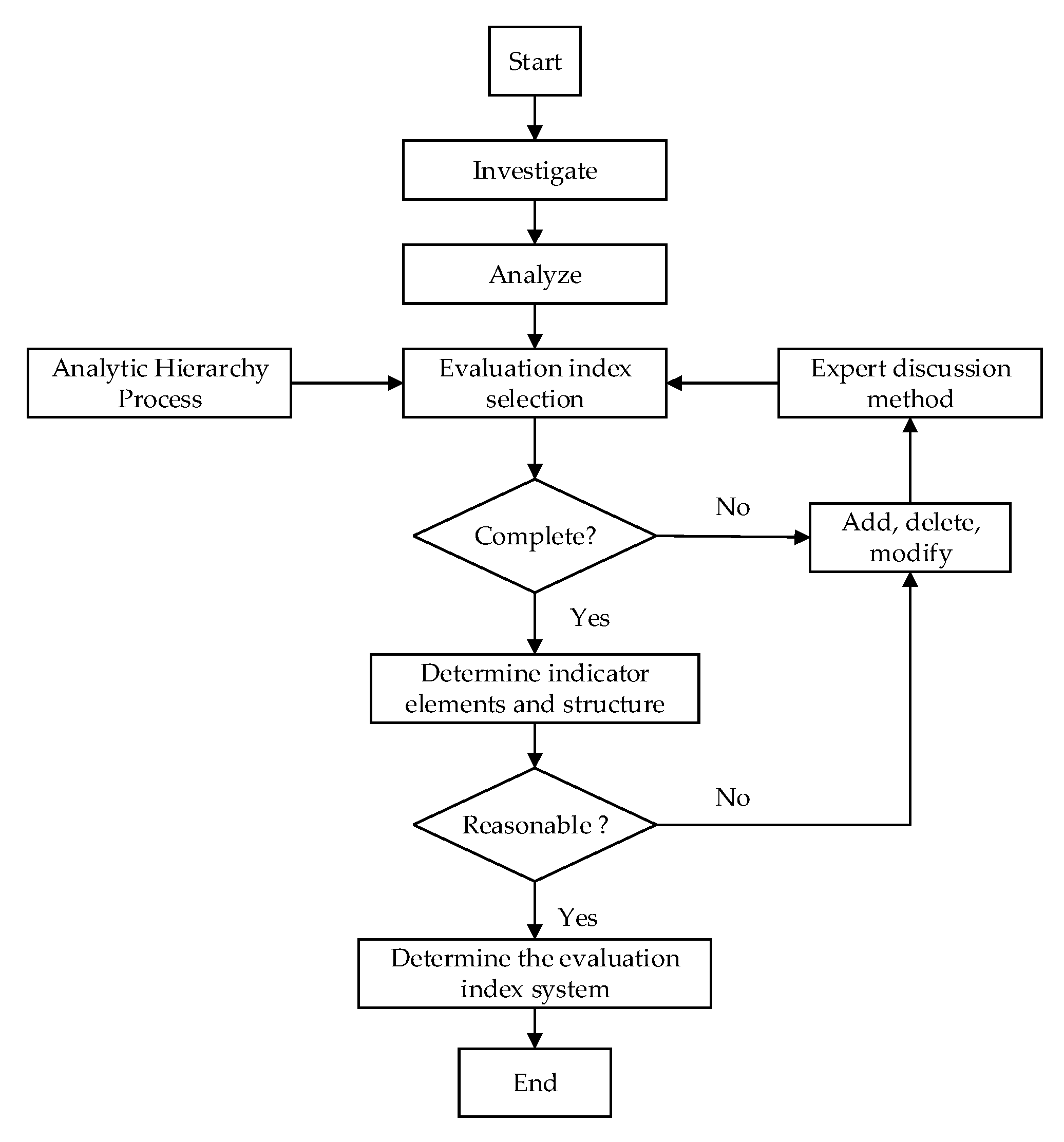
A scientific and reasonable evaluation index is the prerequisite and basis for realizing the quantitative evaluation of the unmanned ship’s obstacle avoidance performance. The process of determining the unmanned ship’s obstacle avoidance performance evaluation index system is shown in Figure 1.

2.1.1. Select Evaluation Index

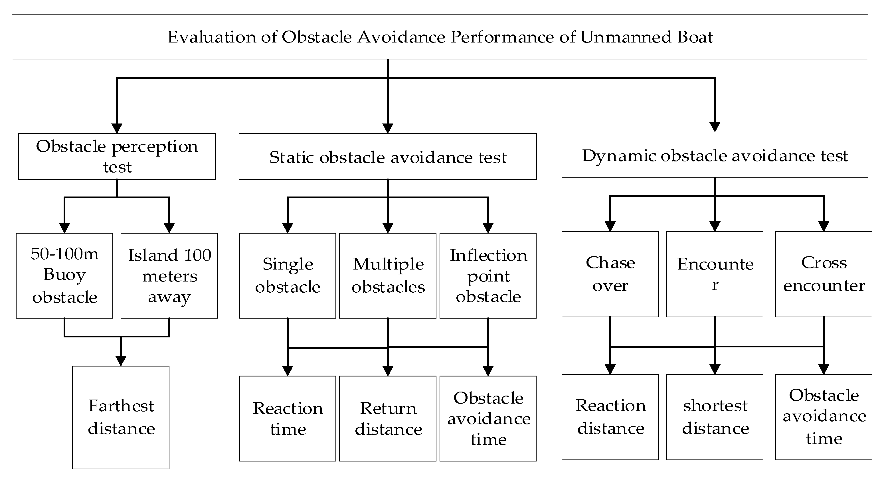
This article refers to the standards of the marine industry and the test specifications for obstacle avoidance of unmanned vehicles. The comprehensive method and analysis method are used to decompose the unmanned ship’s obstacle avoidance performance into various aspects of capability evaluation. The corresponding technical indicators are formulated and analyzed, and the indexes that can reflect the various aspects of the unmanned ship’s obstacle avoidance performance are selected. They are divided into four levels: evaluation objectives, evaluation aspects, evaluation elements and data basis, as shown in Figure 2.

It can be seen from Figure 2 that the evaluation goal is the obstacle avoidance performance of the unmanned ship. The test plan is divided into an obstacle perception test, static obstacle avoidance test and dynamic obstacle avoidance test. Among them, obstacle perception tests include 50–100 m buoy obstacle perception and 100 m away island perception. Static obstacle avoidance tests include a single obstacle test, continuous obstacle test and route turning point obstacle test. The dynamic obstacle avoidance test includes a chasing test, confrontation test, and cross encounter test. Each evaluation aspect also includes the data basis that should be recorded:

(1) Obstacle perception measurement data basis: perception distance.

(2) Static obstacle avoidance measurement data basis: ① reaction distance; ② regression distance; ③ obstacle avoidance time.

(3) Dynamic obstacle avoidance measurement data basis: ① reaction distance; ② minimum distance; ③ obstacle avoidance time.

2.1.2. Determine the Weight of the Evaluation Index

Hierarchical analysis is proposed by Saaty, an American operations planner in the 1970s, and is applicable to the analysis of uncertainty, and the weight of each evaluation index is determined from both qualitative and quantitative dimensions [19]. Based on the selection of technical indicators, the analytic hierarchy process is used to determine the weights of the various evaluation indicators of the unmanned ship’s obstacle avoidance performance.

(1) Build judgment matrix.

From the two aspects of safety and economy, we consider which of the evaluation indexes A_i and A_j of the unmanned ship’s obstacle avoidance performance is more important in the upper layer, its degree of importance, and what value is used to express it. The judgment matrix in the literature [20] is used for reference to define the degree of importance of the unmanned ship’s obstacle avoidance performance evaluation index, as shown in

Table 1. The degree of importance of the evaluation index of the obstacle avoidance performance.

	A1	A2	A3	…	An
A1	a11	a12	a13	…	a1n
A2	a21	a22	a23	…	a2n
A3	a31	a32	a33	…	a3n
…	…	…	…	…	…
An	an1	an2	an3	…	ann

.

The judgment matrix is shown in Formula (1):

$$A={[a_{ij}]}_{n\times n}$$

(1)

From the scale of the judgment matrix, it can be obtained that the judgment matrix A satisfies the following characteristic relations as shown in Formula (2):

$$\{\begin{array}{l}{a}_{ij}>0\\ a_{ii}=1\\ a_{ij}=\frac{1}{a_{ji}}\end{array}$$

(2)

(2) Calculate the weight of the evaluation index of the obstacle avoidance performance of the unmanned ship.

The weight calculation methods include the square root method, the average method, the eigenvector method and the least square method. This paper adopts the eigenvector method to solve the weight vector and the largest eigenvalue of the judgment matrix in (1). The specific solution steps are as follows:

① The judgment matrix A for the evaluation index of the unmanned ship’s obstacle avoidance performance is standardized in columns, and a_ij is transformed into the ratio of this value to the total as follows:

$$\overline{a_{ij}}=\frac{a_{ij}}{{\displaystyle \sum _{i=1}^n{a}_{ij}}}(i,j=1,2,3,\dots ,n)$$

(3)

② Calculate the sum vector of each row of the judgment matrix A as follows:

$$W_i={\displaystyle \sum _{i=1}^n\overline{a_{ij}}}(i,j=1,2,3,\dots ,n)$$

(4)

③ To normalize w_i obtained in (4), obtain the weight vector as follows:

$$\overline{w_i}=\frac{w_i}{{\displaystyle \sum _{i=1}^n{w}_i}}(i=1,2,3,\dots ,n)$$

(5)

④ Solve the largest characteristic root λ_max of the judgment matrix for the evaluation index of the unmanned ship’s obstacle avoidance performance as follows:

$${\lambda }_{\max }={\displaystyle \sum _{i=1}^n\frac{{[A\overline{W_i}]}_i}{n{(\overline{W_i})}_i}}(i,j=1,2,3,\dots ,n)$$

(6)

In order to ensure the consistency of the weight vector to the evaluation logic of each indicator, it is necessary to conduct a consistency test on the maximum eigenvalue so that the weight will not have internal contradictions and ensure the reliability of the evaluation results. The calculation formula of the consistency index CI (consistency index) is shown in Formula (7):

$$CI=\frac{{\lambda }_{\max }-n}{n-1}$$

(7)

Then, we find the consistency index RI; the average random consistency index [21] is shown in

Table 2. Average random consensus index.

n	1	2	3	4	5	6	7	8	9	10	11	12	13	14
RI	0	0	0.52	0.89	1.12	1.24	1.36	1.41	1.46	1.49	1.52	1.54	1.56	1.58

.

Calculate the consistency ratio (CR) as follows:

$$CR=\frac{CI}{RI}$$

(8)

If the CR calculated by Formula (8) is less than 0.1, it can be considered that the judgment matrix is feasible and meets the consistency requirements; otherwise, the judgment matrix should be adjusted to recalculate the weight matrix.

2.2. Quantitative Evaluation Model for the Obstacle Avoidance Performance of Unmanned Ships

Junqing Wei of Carnegie Mellon University’s Department of Electrical and Computer Engineering, among others, proposes an algorithm based on predictive and cost functions to assess driverlessness levels in response to the interaction between cars and the environment on highways [22]. The cost function method is used for the quantitative evaluation of the evaluation factors.

2.2.1. Evaluation Factor Layer Evaluation Model

This layer adopts the cost function method; there are 8 evaluation factors, and a cost function needs to be constructed for each evaluation factor.

① The 50–100 m obstacle sensing.

This factor has only one basic measurement data $d_{longest}$, so the weight value of the basic data is 1. The specified cost function and corresponding evaluation are as follows:

$$c_1=\frac{100}{d_{longest}}=\{\begin{array}{ll}1& excellent\\ (1,1.25]& good\\ (1.25,2]& fair\\ (2,\infty )& poor\end{array}$$

(9)

② The perception of small island 100 m away is as follows:

$$c_2=\frac{100}{d_{longest}}=\{\begin{array}{ll}(0,0.66]& excellent\\ (0.66,1]& good\\ 1& fair\\ (1,\infty )& poor\end{array}$$

(10)

③ Three evaluation factors under static obstacle avoidance.

There are three evaluation factors under static obstacle avoidance: single obstacle static obstacle avoidance, continuous obstacle static obstacle avoidance and inflection point obstacle avoidance. The basic measurement data of these three evaluation factors are the same: they are reaction distance $d_{st}$, regression distance $d^{\prime }{}_{st}$ and obstacle avoidance time $T_{st}$. Therefore, the evaluation model of the three evaluation factors of static obstacle avoidance is the same, and its cost function is composed of the reaction distance, regression distance, obstacle avoidance time and their corresponding weights.

The first is to establish a judgment matrix, using $A_1$, $A_2$ and $A_3$ to represent the reaction distance, return distance and obstacle avoidance time, respectively, and establish the importance relationships, as shown in

Table 3. The importance of the three basic data of static obstacle avoidance.

	$A_1$	$A_2$	$A_3$
$A_1$	1	3	4
$A_2$	1/3	1	2/3
$A_3$	1/4	3/2	1

:

Then, the judgment matrix A is as follows:

$$A=\left\{\begin{array}{ccc}1& 3& 4\\ 1/3& 1& 2/3\\ 1/4& 3/2& 1\end{array}\right\}$$

According to Formula (3), A is normalized by the column as follows:

$$A=\left\{\begin{array}{lll}0.632& 0.545& 0.706\\ 0.211& 0.182& 0.118\\ 0.158& 0.273& 0.176\end{array}\right\}$$

We obtain the weight matrix according to Formulas (4) and (5):

$$\left\{\begin{array}{l}0.627\\ 0.171\\ 0.202\end{array}\right\}$$

We calculate the maximum eigenvalue by Formula (6):

$${\gamma }_{\max }=\frac{1}{3}\times (\frac{1.948}{0.627}+\frac{0.515}{0.171}+\frac{0.615}{0.202})=3.054$$

We calculate the consistency index (CI) according to Formula (7):

$$CI=\frac{{\gamma }_{\max }-n}{n-1}=\frac{3.054-3}{2}=0.027$$

We calculate the consistency ratio (CR) from Table 2 and Formula (8):

$$CR=\frac{CI}{RI}=\frac{0.027}{0.52}=0.052<0.1$$

Therefore, the judgment matrix is reasonable, the weight vector is [0.627, 0.171, 0.202] T, and the three evaluation factors of static obstacle avoidance are the evaluation models of single obstacle static obstacle avoidance, continuous obstacle static obstacle avoidance and inflection point obstacle avoidance as shown in Formula (11):

$$c_3=0.627(-d_{st}+100)+0.171d_{st}+0.202T_{st}$$

(11)

It is stipulated that the ideal state is reached when $d_{st}$ = 100 m, ${d^{\prime }}_{st}$ = 30 m, and $T_{st}$ = 10 s. The corresponding evaluation of the cost function value is shown in Formula (12):

$$c_3=\{\begin{array}{ll}(0,10]& excellent\\ (10,60]& good\\ (60,95]& fair\\ (95,\infty )& poor\end{array}$$

(12)

④ Three evaluation factors for dynamic obstacle avoidance.

The next level of dynamic obstacle avoidance evaluation has three evaluation factors: chase, confrontation and cross encounter. The basic measurement data of these three evaluation factors are reaction distance $d_{dy}$, minimum distance $d_{dy}^{\min }$ and obstacle avoidance time $T_{dy}$. Construct the evaluation model of the three evaluation factors of the next layer of dynamic obstacle avoidance to determine the weight of each basic data. Suppose that the reaction distance, minimum distance and obstacle avoidance time are represented by $A_1$, $A_2$ and $A_3$, respectively, and the importance relationship is established, as shown in

Table 4. The importance of the three basic data of dynamic obstacle avoidance.

	$A_1$	$A_2$	$A_3$
$A_1$	1	3/2	4
$A_2$	2/3	1	2
$A_3$	1/4	1/2	1

:

The judgment matrix A is as follows:

$$A=\left\{\begin{array}{ccc}1& 3/2& 4\\ 2/3& 1& 2\\ 1/4& 1/2& 1\end{array}\right\}$$

Similarly, the weight matrix calculated according to Formulas (3)–(5) is as follows:

$$\left\{\begin{array}{c}0.517\\ 0.359\\ 0.124\end{array}\right\}$$

According to Formulas (6)–(8) and Table 2, the consistency ratio is calculated as follows:

$$CR=0.009<0.1$$

Therefore, the judgment matrix is reasonable, and the weight matrix is [0.517,0.359,0.124] T. The evaluation models of chase, confrontation and cross encounter under dynamic obstacle avoidance are shown in Equation (13):

$$c_4=0.531(-d_{dy}+100)+0.322(-d_{dy}^{\min }+30)+0.147T_{dy}$$

(13)

It is specified that $d_{dy}$ = 100 m, $d_{dy}^{\min }$ = 30 m, and $T_{dy}$ = 6 s to reach the ideal state. The corresponding evaluation of the cost function value is shown in Formula (14):

$$c_4=\{\begin{array}{ll}(0,10]& excellent\\ (10,20]& good\\ (20,50]& fair\\ (50,\infty )& poor\end{array}$$

(14)

2.2.2. Evaluation Model of Evaluation Aspect

The fuzzy comprehensive evaluation method is adopted, and the evaluation is based on the evaluation factors from the evaluation aspects. There are three sets of evaluation aspects: obstacle perception, static obstacle avoidance and dynamic obstacle avoidance. The evaluation models of these three sets are established below.

① Obstacle perception evaluation model.

There are two evaluation factors in the next layer of obstacle perception: ① the longest distance of 50–100 m buoys; and ② the longest distance of 100 islands. Assuming that these two evaluation factors are represented by $q_1$, $q_2$, the evaluation index $Q_{pe}$ set is as follows:

$$Q_{pe}=\{q_1,q_2\}$$

Then, we determine the evaluation set K as follows:

$$K=\{k_1,k_2,k_3,k_4\}$$

Among them, $k_1$ means excellent, $k_2$ means good, $k_3$ means fair, and $k_4$ means poor. Then, we confirm the fuzzy evaluation matrix $S_{pe}$ as follows:

$$S_{pe}=\left[\begin{array}{llll}{s}_{11}& s_{12}& s_{13}& s_{14}\\ s_{21}& s_{22}& s_{23}& s_{24}\end{array}\right]$$

Since there are only two evaluation factors for obstacle perception in the next layer, the weight of these two evaluation factors can be directly obtained: the obstacle perception ability of 50–100 m buoys is more important than the recognition of small islands 100 m away. Under normal circumstances, if the unmanned ship can accurately identify 100 m buoys, it can also accurately identify 100 small islands. Therefore, the weight of the previous evaluation factor is 0.8, and the weight of the latter evaluation factor is 0.2. Thus, the fuzzy comprehensive evaluation model $B_{pe}$ is obtained as shown in Formula (15):

$$B_{pe}=\left(0.8, 0.2\right)\left[\begin{array}{llll}{s}_{11}& s_{12}& s_{13}& s_{14}\\ s_{21}& s_{22}& s_{23}& s_{24}\end{array}\right]$$

(15)

According to Formula (18), the fuzzy comprehensive evaluation score can be calculated.

② Static obstacle avoidance evaluation model

There are three evaluation factors under the static obstacle avoidance layer: single obstacle static obstacle avoidance, continuous obstacle static obstacle avoidance and inflection point obstacle avoidance. Similarly, assuming that these three evaluation factors are represented by $q_1$, $q_2$, and $q_3$, the evaluation index $Q_{st}$ set is as follows:

$$Q_{st}=\left\{q_1, q_2, q_3\right\}$$

Further, the fuzzy evaluation matrix $S_{st}$ is as follows:

$$S_{st}=\left[\begin{array}{llll}{s}_{11}& s_{12}& s_{13}& s_{14}\\ s_{21}& s_{22}& s_{23}& s_{24}\\ s_{31}& s_{32}& s_{33}& s_{34}\end{array}\right]$$

We use the analytic hierarchy process to determine the weight matrix of the three evaluation factors, and list the relationships shown in

Table 5. Relationship of the importance of three evaluation factors of static obstacle avoidance.

	$A_1$	$A_2$	$A_3$
$A_1$	1	1/3	1/2
$A_2$	3	1	5/3
$A_3$	2	3/5	1

, according to the importance of the three evaluation factors. Among them, $A_1$ is the static obstacle avoidance of a single obstacle, $A_2$ is the static obstacle avoidance of continuous obstacles, and $A_3$ is the static obstacle avoidance of inflection point obstacles.

Then, the judgment matrix A is as follows:

$$A=\left\{\begin{array}{ccc}1& 1/3& 1/2\\ 3& 1& 5/3\\ 2& 3/5& 1\end{array}\right\}$$

According to Formulas (3)–(5), the calculated weight matrix is as follows:

$$\left\{\begin{array}{l}0.165\\ 0.515\\ 0.320\end{array}\right\}$$

According to Formulas (6)–(8) and Table 2, the consistency ratio is calculated as follows:

$$CR\approx 0.002<0.1$$

Therefore, the weight matrix obtained is reasonable, the weight matrix is [0.165, 0.515, 0.320] T, and the static obstacle avoidance fuzzy comprehensive evaluation model $B_{st}$ is further obtained, according to Equation (15) as shown in Equation (16):

$$B_{st}=\left(0.165, 0.515, 0.320\right)\left[\begin{array}{llll}{s}_{11}& s_{12}& s_{13}& s_{14}\\ s_{21}& s_{22}& s_{23}& s_{24}\\ s_{31}& s_{32}& s_{33}& s_{34}\end{array}\right]$$

(16)

Similarly, the static obstacle avoidance comprehensive score can be calculated according to Formula (8).

③ Dynamic obstacle avoidance evaluation model.

There are three evaluation factors under the dynamic obstacle avoidance layer: chasing dynamic obstacle avoidance, confrontation dynamic obstacle avoidance and cross encounter. Similarly, assuming that these three evaluation factors are represented by $q_1$, $q_2$, and $q_3$, the evaluation index $Q_{dy}$ set is as follows:

$$Q_{dy}=\left\{q_1, q_2 ,q_3\right\}$$

Further, the fuzzy evaluation matrix $S_{dy}$ is as follows:

$$S_{dy}=\left[\begin{array}{llll}{s}_{11}& s_{12}& s_{13}& s_{14}\\ s_{21}& s_{22}& s_{23}& s_{24}\\ s_{31}& s_{32}& s_{33}& s_{34}\end{array}\right]$$

We use the analytic hierarchy process to determine the weight matrix of the three evaluation factors. According to the importance of these three evaluation factors, the relationships shown in

Table 6. Relationship of the importance of three evaluation factors of dynamic obstacle avoidance.

	$A_1$	$A_2$	$A_3$
$A_1$	1	2/3	1/2
$A_2$	3/2	1	3/5
$A_3$	2	5/3	1

are listed. Among them, $A_1$ is the dynamic obstacle avoidance of chasing and crossing, $A_2$ is the dynamic obstacle avoidance of confrontation, and $A_3$ is the dynamic obstacle avoidance of cross encounter.

Then, the judgment matrix A is as follows:

$$A=\left\{\begin{array}{ccc}1& 2/3& 1/2\\ 3/2& 1& 3/5\\ 2& 5/3& 1\end{array}\right\}$$

According to Formulas (3)–(5), the calculated weight matrix is as follows:

$$\left\{\begin{array}{l}0.220\\ 0.306\\ 0.474\end{array}\right\}$$

According to Formulas (6)–(8) and Table 2, the consistency ratio is calculated as follows:

$$CR\approx 0.005<0.1$$

Therefore, the weight matrix obtained is reasonable, the weight matrix is [0.220, 0.306, 0.474] T, and the static obstacle avoidance fuzzy comprehensive evaluation model $B_{dy}$ is further obtained, according to Equation (15) as shown in Equation (17):

$$B_{dy}=\left(0.220, 0.306, 0.474\right)\left[\begin{array}{llll}{s}_{11}& s_{12}& s_{13}& s_{14}\\ s_{21}& s_{22}& s_{23}& s_{24}\\ s_{31}& s_{32}& s_{33}& s_{34}\end{array}\right]$$

(17)

Similarly, the dynamic obstacle avoidance comprehensive score can be calculated, according to Formula (8).

2.3. Software for Quantitative Evaluation of Unmanned Ship’s Obstacle Avoidance Performance

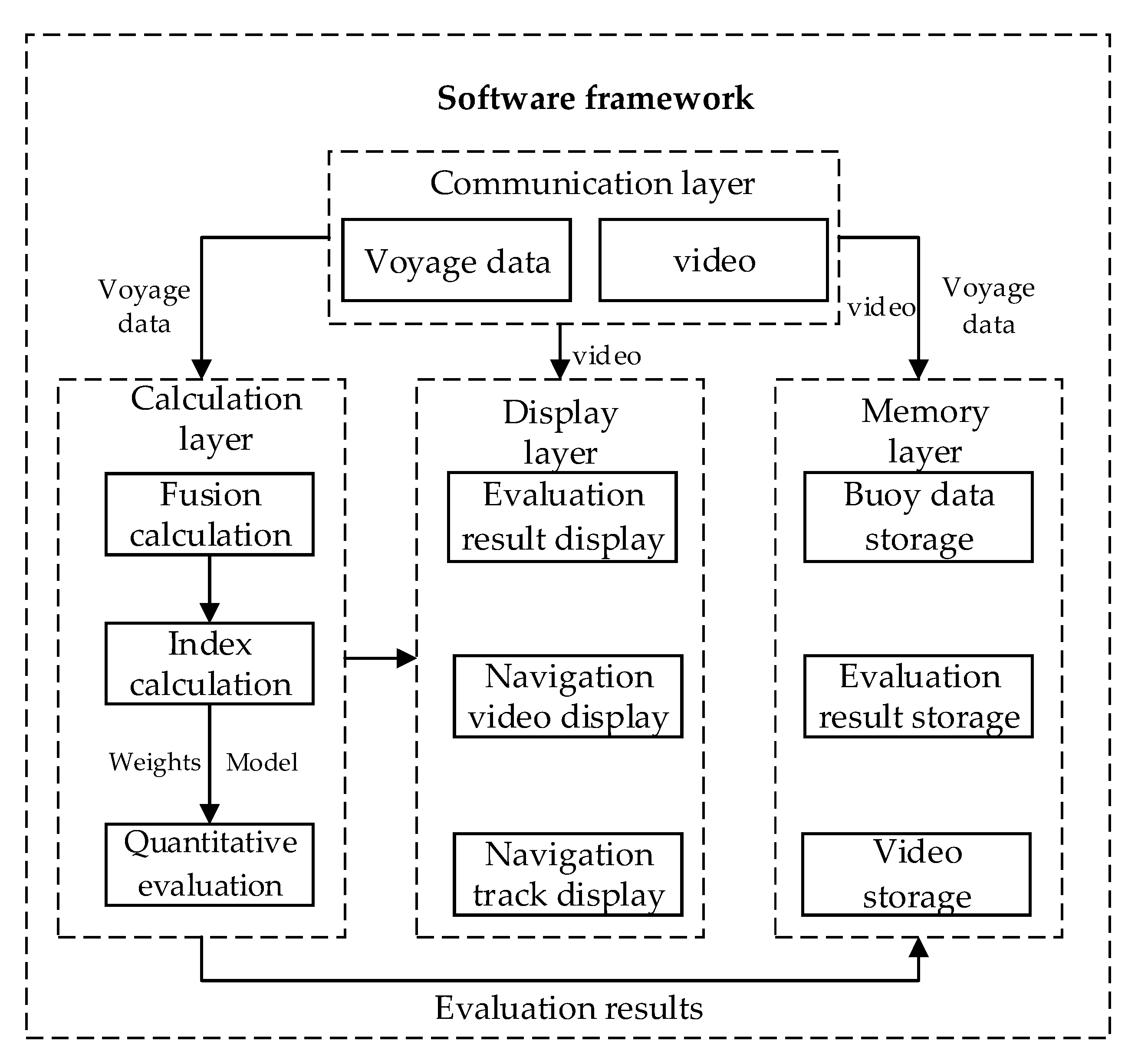
The software for quantitative evaluation of unmanned ship’s obstacle avoidance performance is located in the shore-based data processing center, which completes the function of index calculation, quantitative evaluation result display and data storage, and realizes the paperless traceability test of an unmanned ship’s obstacle avoidance performance.

The software for the quantitative evaluation of the obstacle avoidance performance of the unmanned ship is divided into four parts, namely, the calculation layer, the display layer, the storage layer and the communication layer. The software framework is shown in Figure 3.

3. Obstacle Avoidance Performance Test Results and Evaluation of Unmanned Ships

Based on the mobile buoy measurement and control system, the unmanned ship navigation monitoring experiment and obstacle avoidance performance test experiment are carried out to verify the effectiveness of the test system. The experiments were all carried out in the coastal waters of Longxue Island, Guangzhou. The test site was 900 m long, 800 m wide, and 8 m deep. A mobile buoy was arranged in the test site. Through the unmanned ship navigation monitoring experiment, the effectiveness of the buoy measurement and control system and the unmanned ship navigation monitoring method was verified. We used the test system to test the obstacle avoidance performance of the unmanned ship in the test sea area and quantitatively evaluated the obstacle avoidance performance of the unmanned ship from the three aspects of obstacle perception, static obstacle avoidance and dynamic obstacle avoidance.

The obstacle perception test experiments include unmanned ships to identify buoy obstacles in the range of 0–100 m, and unmanned ships to identify small islands 100 m away. The former places the buoy as an obstacle in the test sea area, and measures the size of the unmanned ship on the sea surface in the test sea area in advance, which is about 1.51 m × 1.51 m × 2.10 m. The diameter of the buoy base is 1.51 m, and the specified error is within 0.2 diameter length as a reasonable error range [23], that is, the allowable error is 0.3 m. The experiment was carried out 3 times, and in the three sets of experiments, the tested unmanned craft could accurately identify the buoy when the distance was less than 90 m, 70 m, and 70 m. In the second and third experiments, at distances greater than 70 m, the recognition distance began to be greater than 0.3 m, but the actual difference was different: the second and third differences were 0.51 m and 2.91 m, respectively.

The basic measurement data for this test were 90 m, 70 m, and 70 m, respectively. Using the cost function method, we can calculate the distance cost value of the measured unmanned ships’ identification buoy according to Formula (9), as shown in Formula (18):

$$c_1=\frac{100}{d_{longest}}=\{\begin{array}{ll}\frac{100}{90}\approx 1.11& group1\\ \frac{100}{70}\approx 1.43& group2\\ \frac{100}{70}\approx 1.43& group3\end{array}$$

(18)

In the island identification test, the unmanned ship first sails to a designated area about 100 m away from the island, and the unmanned ship sends the measured distance and azimuth of the island to the shore base for comparison with the actual distance and azimuth. The specified distance error is 0.2 island width as a reasonable range [24], that is, the distance error is not more than 1.5 m. The experiment measured the distances for the unmanned ship to identify the islands as being 110 m, 105 m, and 100 m respectively, that is, the basic measurement data for this test were 110 m, 105 m, and 100 m, respectively. Using the cost function method, according to Formula (10), we can calculate the cost value of the unmanned ship to identify the longest distance of the island as shown in Formula (19):

$$c_2=\frac{100}{d_{longest}}=\{\begin{array}{ll}\frac{100}{110}\approx 0.909& group1\\ \frac{100}{105}\approx 0.952& group2\\ \frac{100}{100}\approx 1& group3\end{array}$$

(19)

The static obstacle test is divided into the single obstacle avoidance test, continuous obstacle avoidance test and inflection point obstacle test [25]. During the test, the buoy appeared on the path of the unmanned ship, and the unmanned ship did not know the latitude and longitude of the position of the buoy in advance. The experiment was carried out 3 times to calculate the cost function values of single obstacle static obstacle avoidance, continuous obstacle static obstacle avoidance, and inflection point obstacle static obstacle avoidance as shown in Formulas (20)–(22).

$$\begin{array}{ll}{c}_{alo}& =0.627(-d_{st}+100)+0.171d_{st}^{\prime }+0.202T_{st}\\ & =\{\begin{array}{ll}74.81& group1\\ 86.02& group2\\ 53.25& group3\end{array}\end{array}$$

(20)

$$\begin{array}{ll}{c}_{con}& =0.627(-d_{st}+100)+0.171d_{st}^{\prime }+0.202T_{st}\\ & =\{\begin{array}{ll}77.14& group1\\ 57.93& group2\\ 60.33& group3\end{array}\end{array}$$

(21)

$$\begin{array}{ll}{c}_{tp}& =0.627(-d_{st}+100)+0.171d_{st}^{\prime }+0.202T_{st}\\ & =\{\begin{array}{ll}47.61& group1\\ 58.61& group2\\ 72.63& group3\end{array}\end{array}$$

(22)

The dynamic obstacle test mainly includes three experimental scenarios: chasing, confrontation, and cross encounter. From these three aspects, the obstacle avoidance performance of the unmanned ship was tested, according to the test plan. After the unmanned ship starts to sail, each buoy records the unmanned ship’s navigation data and sends it to the shore. After shore-based fusion, the navigation trajectory of the unmanned ship and the navigation trajectory of the dynamic obstacle buoy are displayed on the satellite map, and the response distance, minimum distance, and obstacle avoidance time are calculated. The experimental results are shown in

Table 7. Basic measurement data for obstacle avoidance of unmanned ships in chasing scenes.

Number of Experimental Groups	1	2	3
Latitude and longitude of the unmanned ship/(starting time of obstacle avoidance)	113.646286, 22.705751	113.646339, 22.703392	113.643262, 22.705313
Latitude and longitude of buoy/(starting time of obstacle avoidance)	113.646337, 22.705592	113.646240, 22.703587	113.643575, 22.705310
Latitude and longitude of the unmanned ship/(the closest time to the buoy)	113.646492, 22.705194	113.646003, 22.703581	113.643611, 22.705494
Latitude and longitude of the buoy/(the shortest time between the unmanned ship and the buoy)	113.646490, 22.705226	113.646182, 22.703703	113.643683, 22.705221 s
Reaction distance/m	18.41	23.91	32.12
Shortest distance/m	3.48	22.56	31.20
Obstacle avoidance time/s	14	27	30

,

Table 8. Basic measurement data for obstacle avoidance of unmanned ships in encounter scenarios.

Number of Experimental Groups	1	2	3
Latitude and longitude of the unmanned ship/(starting time of obstacle avoidance)	113.645536, 22.705532	113.646194, 22.705171	113.645604, 22.703470
Latitude and longitude of buoy/(starting time of obstacle avoidance)	113.645501, 22.705082	113.646208, 22.704783	113.645936, 22.703452
Latitude and longitude of the unmanned ship/(the closest time to the buoy)	113.645680, 22.705375	113.646351, 22.705005	113.645819, 22.703605
Latitude and longitude of the buoy/(the shortest time between the unmanned ship and the buoy)	113.645523. 22.705349	113.646208, 22.704992	113.645806, 22.703443
Reaction distance/m	50.02	43.09	34.12
Shortest distance/m	16.37	14.74	18.04
Obstacle avoidance time/s	38	22	24

and

Table 9. Basic measurement data for obstacle avoidance of unmanned ships in cross-encounter scenarios.

Number of Experimental Groups	1	2	3
Latitude and longitude of the unmanned ship/(starting time of obstacle avoidance)	113.646240, 22.703484	113.643329, 22.705859	113.644704, 22.705209
Latitude and longitude of buoy/(starting time of obstacle avoidance)	113.647049, 22.703447	113.643656, 22.705590	113.645335, 22.704818
Latitude and longitude of the unmanned ship/(the closest time to the buoy)	113.646621, 22.703270	113.643329, 22.705859	113.645093, 22.705254
Latitude and longitude of the buoy/(the shortest time between the unmanned ship and the buoy)	113.647082, 22.703404	113.643665, 22.705724	113.645053, 22.705248
Reaction distance/m	83.11	44.91	77.94
Shortest distance/m	49.59	37.59	4.17
Obstacle avoidance time/s	26	22	10

.

According to the evaluation model in Formula (13), calculate the corresponding result cost function value of the dynamic obstacle avoidance test experiment of chase, confrontation, and cross encounter $c_{chase}, c_{against}, c_{cross}$, as shown in Formulas (23)–(25):

$$\begin{array}{ll}{c}_{chase}& =0.531(-d_{dy}+100)+0.322(-d_{dy}^{\min }+30)+0.147T_{dy}\\ & =\{\begin{array}{ll}53.92& group1\\ 46.77& group2\\ 40.07& group3\end{array}\end{array}$$

(23)

$$\begin{array}{ll}{c}_{against}& =0.531(-d_{dy}+100)+0.322(-d_{dy}^{\min }+30)+0.147T_{dy}\\ & =\{\begin{array}{ll}36.51& group1\\ 38.37& group2\\ 44.36& group3\end{array}\end{array}$$

(24)

$$\begin{array}{ll}{c}_{cross}& =0.531(-d_{dy}+100)+0.322(-d_{dy}^{\min }+30)+0.147T_{dy}\frac{1}{2}\\ & =\{\begin{array}{ll}6.48& group1\\ 30.04& group2\\ 21.50& group3\end{array}\end{array}$$

(25)

The unmanned ship obstacle avoidance performance test experiment is completed. Through the cost function method combined with the basic measurement data calculated in the experimental process, each evaluation factor of the evaluation factor layer is evaluated. Furthermore, the fuzzy comprehensive evaluation method can be used to quantitatively evaluate the obstacle avoidance performance of the unmanned ship in the three evaluation aspects of obstacle perception, static obstacle avoidance and dynamic obstacle avoidance.

(1) Quantitative evaluation of obstacle perception performance.

According to Equations (9) and (10), the two evaluation factors of obstacle perception in the next layer are the obstacle perception of 50–100 m buoy and the perception of small islands beyond 100 m. The performance in this experiment is {“good”, “fair”, “fair”}, {“good”, “good”, “fair”}, and the quantitative evaluation of obstacle perception performance in this experiment can be obtained from Equation (15) for the following:

$$B_{pe}=\left(0.8, 0.2\right)\left[\begin{array}{llll}0& \frac{1}{3}& \frac{2}{3}& 0\\ 0& \frac{2}{3}& \frac{1}{3}& 0\end{array}\right]=\left[0 0.4 0.6 0\right]$$

(26)

For the obstacle perception performance of the tested unmanned ship, the membership degree of “good” is 0.4, and the membership degree of “fair” is 0.6. According to Equation (8), the obstacle perception performance score can be obtained as shown in Equation (27):

$$scor{e}_{pe}=100\times \left(0.8\times 0.4+0.6\times 0.6\right)=68$$

(27)

(2) Quantitative evaluation of static obstacle avoidance performance.

According to Formula (12), the three evaluation factors of the next layer of static obstacle avoidance are single obstacle static obstacle avoidance, continuous obstacle static obstacle avoidance and inflection point obstacle static obstacle avoidance. The performance in this experiment is {“fair”, “fair”, “good”}, {“fair”, “good”, “fair”}, {“good”, “good”, “fair”}. From Equation (16), the quantitative evaluation of static obstacle avoidance performance in this experiment is shown in Equation (28):

$$B_{st}=\left(0.165, 0.515, 0.320\right)\left[\begin{array}{llll}0& \frac{1}{3}& \frac{2}{3}& 0\\ 0& \frac{1}{3}& \frac{2}{3}& 0\\ 0& \frac{2}{3}& \frac{1}{3}& 0\end{array}\right]=\left[0 0.44 0.56 0\right]$$

(28)

In the evaluation of the static obstacle avoidance performance of the tested unmanned ship, the membership degree that is good is 0.44, and the membership degree that is “fair” is 0.56. According to Equation (8), the static obstacle avoidance performance score can be obtained as shown in Equation (29):

$$scor{e}_{st}=100\times \left(0.8\times 0.44+0.6\times 0.56\right)=68.8$$

(29)

(3) Quantitative evaluation of dynamic obstacle avoidance performance.

According to Formula (14), the three evaluation factors of the next layer of dynamic obstacle avoidance are the performance of chasing dynamic obstacle avoidance, facing dynamic obstacle avoidance and cross encounter dynamic obstacle avoidance performance. The performances in this experiment are {“poor”, “fair”, “fair”}, {“fair”, “fair”, “fair”}, {“excellent”, “fair”, “fair”}. From Equation (17), the quantitative evaluation of dynamic obstacle avoidance performance in this experiment is shown in Equation (30):

$$B_{dy}=\left(0.220, 0.306, 0.474\right)\left[\begin{array}{llll}0& 0& \frac{2}{3}& \frac{1}{3}\\ 0& 0& 1& 0\\ \frac{1}{3}& 0& \frac{2}{3}& 0\end{array}\right]=\left[0.158 0 0.769 0.073\right]$$

(30)

In the dynamic obstacle avoidance performance evaluation of the tested unmanned ship, the membership degree of “excellent” is 0.158, the membership degree of “fair” is 0.769, and the membership degree of “poor” is 0.073. According to Formula (8), the dynamic obstacle avoidance performance score can be obtained as shown in Formula (31):

$$scor{e}_{dy}=100\times \left(1\times 0.158+0.6\times 0.769+0.3\times 0.073\right)=64.13$$

(31)

In summary, in this test, the unmanned ship’s obstacle perception performance score is 68, the static obstacle avoidance performance score is 68.8, and the dynamic obstacle avoidance performance score is 64.13.

(4) Analysis of test results.

From the test results, the obstacle perception, static obstacle avoidance and dynamic obstacle avoidance performance scores of the tested unmanned ships are 68, 68.8, and 64.13, respectively. According to the evaluation set in Chapter 5, the score can be specified with (90,100) as “excellent”, (80,90) as “good”, (60,80) as “fair”, and 60 points or less as “poor”. Therefore, the three evaluation aspects of the unmanned ship’s obstacle avoidance performance are rated as “fair”. In the obstacle perception test, the longest distances at which the unmanned ship can identify buoys are 90 m, 70 m, and 70 m respectively. Reach the ideal level of 0.9, 0.7, and 0.7. The corresponding evaluations of the scores are “good”, “fair”, and “fair”, which is more reasonable. In the small island identification test, the unmanned ship can accurately identify small islands at 110 m, 105 m, and 100 m, indicating that the ability to perceive large objects is better. Since the proportion of the sensing buoy is 4 times the proportion of the sensing island, it is finally corresponding to “fair”, according to the test score, and the performance of sensing small objects at sea needs to be further improved.

In the static obstacle avoidance test, the return distance of the unmanned ships in the previous two single-obstacle static obstacle avoidance tests was too large and the obstacle avoidance time was too long, which resulted in the evaluation as “fair”. This was improved at the third time, and the score improved. In the continuous static obstacle avoidance, the score was also affected by the regression distance problem for the first time, and the score improved after the last two improvements. The inflection point obstacle test is relatively simple. The unmanned ship performed well in the first two tests, but the return distance increased in the third time, and the response distance with a larger proportion was also reduced, which ultimately lowered the score by one level. According to the proportions of the three groups of test items [0.165, 0.515, 0.320], the final score calculated corresponds to “fair”. The response distance of the unmanned ship in static obstacle avoidance can be appropriately increased, and the return distance should be optimized and reduced.

In the dynamic obstacle avoidance test, the minimum distance of the unmanned ship from the buoy in the first overtake scene test was 3.18 m, which was less than the width of the unmanned ship, which resulted in the score of this test being “poor”. This was adjusted for the last two times, and the corresponding performance evaluation was changed to “fair”. In the face-to-face test, the basic data in the three tests of the unmanned ship were relatively stable, and all the basic data were in the range of 0.3 to 0.5 in the ideal situation; the corresponding evaluations were all at the “fair” level. In the cross-encounter scenario test, the unmanned ship adopted three different strategies to avoid obstacles. For the first time, the method of sailing around behind the buoy was adopted. The reaction distance was the farthest, and the obstacle avoidance time was earlier. This not only avoided collisions, but also saved obstacle avoidance time under safe conditions. The corresponding evaluation was “excellent”. In the second test, the unmanned ship used a method of slowing down until it stopped sailing to avoid the buoy. This method was conservative and ensured safety, but the response distance was the smallest among the three sets of tests, and the final evaluation was “fair”. In the third test, the unmanned ship used the acceleration method to accelerate at a far distance, and finally completed the dynamic obstacle avoidance. The response distance of the unmanned craft in this test was far, which made up for the shortcoming of the small minimum distance, and the corresponding evaluation of the score was “fair”. According to the proportions of these three groups of test items [0.220, 0.306, 0.474], the calculated score finally corresponds to “fair”. According to the evaluation results, the obstacle avoidance strategy of the unmanned ship can be improved; for example, the response distance of the unmanned ship’s dynamic obstacle avoidance can be appropriately increased.

4. Conclusions

This article is mainly aimed at the needs of the evaluation of the obstacle avoidance performance of the unmanned ship. A quantitative evaluation model was established to evaluate quantitatively the obstacle perception performance, static obstacle avoidance performance and dynamic obstacle avoidance performance of an unmanned ship.

(1) By analyzing the evaluation indicators of unmanned ships, the obstacle avoidance performance of the unmanned ship is evaluated in layers. The analytic hierarchy process is used to assign weights to the selected indicators. Then, the cost function method and fuzzy comprehensive evaluation method are combined to establish a quantitative evaluation model of the unmanned ship’s obstacle avoidance performance.

(2) Based on the established quantitative evaluation model, a 50~100 m buoy obstacle perception test and 100 m away island perception test are carried out. A quantitative evaluation score of 68 points for the obstacle perception performance of the tested unmanned ship is obtained. Using buoys as static obstacles, the obstacle avoidance performance of single obstacles, continuous obstacles and inflection point obstacles are evaluated, respectively. The obtained static obstacle avoidance performance quantitative evaluation score is 68.8 points. With buoys as dynamic obstacles, the performance evaluation of obstacle avoidance in chasing, facing and crossing encounters is carried out, respectively. The obtained quantitative evaluation score of dynamic obstacle avoidance performance is 64.13 points. The above results verify the rationality of the quantitative evaluation model, which can provide reference for the quantitative evaluation and the improvement of the unmanned ship’s obstacle avoidance performance.

References

- Kang, M.; Kwon, S.; Park, J.; Kim, T.; Han, J.; Wang, J.; Hong, S.; Shim, Y.; Yoon, S.; Yoo, B.; et al. Development of USV Autonomy for the 2014 Maritime RobotX Challenge. IFAC-PapersOnLine 2015, 48, 13–18. [Google Scholar] [CrossRef]
- Hong, X.; Wei, X.; Huang, Y.; Liu, Y.; Xiao, G. Local path planning method for unmanned ships combining image recognition and VFH+. J. South China Univ. Technol. (Nat. Sci. Ed.) 2019, 47, 24–33. [Google Scholar]
- Kim, H.G.; Yun, S.J.; Choi, Y.H.; Ryu, J.K.; Suh, J.H. Collision Avoidance Algorithm Based on COLREGs for Unmanned Surface Vehicle. J. Mar. Sci. Eng. 2021, 9, 863. [Google Scholar] [CrossRef]
- Hu, Y.; Zhang, A.; Tian, W.; Zhang, J.; Hou, Z. Multi-Ship Collision Avoidance Decision-Making Based on Collision Risk Index. J. Mar. Sci. Eng. 2020, 8, 640. [Google Scholar] [CrossRef]
- Ahmed, Y.A.; Hannan, M.A.; Oraby, M.Y.; Maimun, A. COLREGs Compliant Fuzzy-Based Collision Avoidance System for Multiple Ship Encounters. J. Mar. Sci. Eng. 2021, 9, 790. [Google Scholar] [CrossRef]
- Phanthong, T.; Maki, T.; Ura, T.; Sakamaki, T.; Aiyarak, P. Application of A* algorithm for real-time path re-planning of an unmanned surface vehicle avoiding underwater obstacles. J. Mar. Sci. Appl. 2014, 13, 105–116. [Google Scholar] [CrossRef]
- Caccia, M.; Bibuli, M.; Bono, R.; Bruzzone, G. Basic navigation, guidance and control of an unmanned surface vehicle. Auton. Robot. 2008, 25, 349–365. [Google Scholar] [CrossRef]
- Liu, Y.; Bucknall, R. Path planning algorithm for unmanned surface vehicle formations in a practical maritime environment. Ocean. Eng. 2015, 97, 126–144. [Google Scholar] [CrossRef]
- Villa, J.; Aaltonen, J.; Koskinen, K.T. Path-following with lidar-based obstacle avoidance of an unmanned surface vehicle in harbor conditions. IEEE Trans. Mechatron. 2020, 25, 1812–1820. [Google Scholar] [CrossRef]
- Švec, P.; Thakur, A.; Raboin, E.; Shah, B.C.; Gupta, S.K. Target following with motion prediction for unmanned surface vehicle operating in cluttered environments. Auton. Robot. 2014, 36, 383–405. [Google Scholar] [CrossRef]
- Meyer, E.; Heiberg, A.; Rasheed, A.; San, O. COLREG-Compliant Collision Avoidance for Unmanned Surface Vehicle Using Deep Reinforcement Learning. IEEE Access 2020, 8, 165344–165364. [Google Scholar] [CrossRef]
- Anonymous. China opens the world’s largest unmanned ship marine test site. China Inf. Circ. 2018, 16, 52. [Google Scholar]
- Anonymous. China Classification Society awarded Shanghai Jiaotong University a certificate of service provider approval for unmanned ship test site. China Ship Insp. 2019, 21, 2. [Google Scholar]
- Anonymous. The opening of the first National Intelligent Unmanned Ship Search and Rescue Competition. Navig. Technol. 2020, 42, 16. [Google Scholar]
- Mu, H. Research on demand demonstration of unmanned ship comprehensive test and evaluation test site at sea. China Shipbuild. 2020, 61, 164–172. [Google Scholar]
- Wang, H.; Huang, Y.; Zhao, K.; Yi, H. The construction of a test field for intelligent ships in real seas urgently needs joint efforts. China Ship Insp. 2020, 22, 64–67. [Google Scholar]
- Xiao, G.; Tong, C.; Wang, Y.; Guan, S.; Hong, X.; Shang, B. CFD Simulation of the Safety of Unmanned Ship Berthing under the Influence of Various Factors. Appl. Sci. 2021, 11, 7102. [Google Scholar] [CrossRef]
- Pu, H.; Ding, F.; Li, X.; Luo, J.; Peng, Y. Dynamic obstacle avoidance method for unmanned craft based on elliptical collision cone. Chin. J. Sci. Instrum. 2017, 38, 1756–1762. [Google Scholar]
- Deng, X.; Li, J.; Zeng, H.; Chen, J.; Zhao, J. Analysis of the weight calculation method of hierarchical analysis method and its application research. Pract. Underst. Math. 2012, 42, 93–100. [Google Scholar]
- Liu, P.; Dong, Z.; Qu, Y.; Zhang, U. Evaluation of equipment maintenance and support capability based on AHP and fuzzy comprehensive evaluation. Tactical Missile Technol. 2012, 33, 47–50. [Google Scholar]
- Wang, Q. Study on the risk of subway crowded stampede accident based on the method of empowerment correlation. J. Chin. J. Saf. Sci. 2013, 23, 94–100. [Google Scholar]
- Wei, J.; Dolan, J.M.; Litkouhi, B. A prediction-and cost function-based algorithm for robust autonomous freeway driving. In Proceedings of the 2010 IEEE Intelligent Vehicles Symposium, La Jolla, CA, USA, 21–24 June 2010; pp. 512–517. [Google Scholar]
- Ship Industry Standard. CB/T 3970-2005, DGPS Test Method for Ship Speed and Maneuverability; Ship Industry Standard: Beijing, China, 2005. [Google Scholar]
- Ship Industry Standard. CB/Z 191-1996, Test Method pf Real Surface Ship Maneuverability; Shipbuilding Industry Standard: Beijing, China, 1996. [Google Scholar]
- Guangzhou Innovative Intelligent Unmanned Vessel Technology Research Institute. Q/GIIUV X03-2019, Test Method for Static Obstacle Avoidance Performance of Unmanned Vessel; Guangzhou Innovative Intelligent Unmanned Vessel Technology Research Institute: Guangzhou, China, 2019. [Google Scholar]
Publisher’s Note: MDPI stays neutral with regard to jurisdictional claims in published maps and institutional affiliations. |
© 2021 by the authors. Licensee MDPI, Basel, Switzerland. This article is an open access article distributed under the terms and conditions of the Creative Commons Attribution (CC BY) license (https://creativecommons.org/licenses/by/4.0/).