Article

Unsteady Linearisation of Bed Shear Stress for Idealised Storm Surge Modelling

by
Pieter C. Roos
1,*,
Giordano Lipari
2,
Chris Pitzalis
3,
Koen R. G. Reef
1,
Gerhardus H. P. Campmans
1 and
Suzanne J. M. H. Hulscher
1
1
Water Engineering & Management, Faculty of Engineering Technology, University of Twente, P.O. Box 217, 7500 AE Enschede, The Netherlands
2
Watermotion | Waterbeweging, Zwolle, The Netherlands
3
Flood Management, Arcadis Nederland B.V., P.O. Box 264, 6800 AG Arnhem, The Netherlands
*
Author to whom correspondence should be addressed.
J. Mar. Sci. Eng. 2021, 9(11), 1160; https://doi.org/10.3390/jmse9111160
Submission received: 18 August 2021 / Revised: 24 September 2021 / Accepted: 4 October 2021 / Published: 21 October 2021

Abstract

:
The modelling of time-varying shallow flows, such as tides and storm surges, is complicated by the nonlinear dependency of bed shear stress on flow speed. For tidal flows, Lorentz’s linearisation circumvents nonlinearity by specifying a (steady) friction coefficient r based on a tide-averaged criterion of energy equivalence. However, this approach is not suitable for phenomena with episodic and irregular forcings such as storm surges. Here, we studied the implications of applying Lorentz’s energy criterion in an instantaneous sense, so that an unsteady friction coefficient r ( t ) adjusts to the temporal development of natural wind-driven flows. This new bed-stress parametrisation was implemented in an idealised model of a single channel, forced by time-varying signals of wind stress (acting over the entire domain) and surface elevation (at the channel mouth). The solution method combines analytical solutions of the cross-sectionally averaged linearised shallow-water equations, obtained in the frequency domain, with an iterative procedure to determine r ( t ) . Model results, compared with a reference finite-difference solution retaining the quadratic bed shear stress, show that this new approach accurately captures the qualitative and quantitative aspects of the surge dynamics (height and timing of surge peaks, sloshing, friction-induced tide-surge interaction) for both synthetic and realistic wind forcings.

1. Introduction

Bottom friction is important for shallow water flows, e.g., those associated with tides and storm surges in the marine environment, as discussed in [1]. The nonlinear dependency of bed shear stress on flow speed contributes to various phenomena such as tide-surge interactions [2,3] and the deformation of tidal curves [1]. In many natural systems, bottom friction even acts as the dominant source of nonlinearity, as is the case for the Thames Estuary, UK; see [2].
At the same time, this nonlinearity may complicate solution techniques in process-based models. This is particularly the case for the subclass of idealised or exploratory process-based models, e.g., [4], which aim to study physical phenomena in isolation. These models usually schematise processes and geometry, thus enabling one to determine the analytical solution to (parts of) the problem, which in turn allows for rapid extensive sensitivity analyses.
The nonlinearity of the bed shear stress can be circumvented by a linearisation that simplifies the solution while being physically acceptable for the problem under consideration. Assuming one-dimensional channel flow, with cross-sectionally averaged velocity u and bed shear stress τ b , the linearisation can be written as
τ b ρ = c d | u | u r u ,
where ρ is the water density, c d is the dimensionless drag coefficient of the conventional quadratic stress parametrisation, here assumed to be constant, and r is the linear friction coefficient (in m s 1 ).
For tidal flows, Lorentz [5,6] first proposed such a linearisation. He specified the (steady) friction coefficient r by requiring that the energy dissipated by the bottom friction per unit of bed area over a tidal cycle T, τ b d t , is equal for both parametrisations in Equation (1). Assuming a monochromatic tidal flow signal u = U cos ω t with angular frequency ω = 2 π / T and (yet unknown) amplitude U, this gives
r = 8 c d U 3 π ( f o r   t i d a l   f l o w s ) .
The combination of Equations (1) and (2) is known as Lorentz’s linearisation, also referred to as equivalent linearisation [7]. Two caveats are in order, e.g., [8].
  • Equation (2) can be applied locally, leading to an r-value valid at a single point in the model domain. However, to facilitate analytical solution, the friction coefficient r is often assumed to be spatially uniform over the model domain (or over subdomains); the energy criterion introduced above should then be applied in a spatially integrated sense. This implies that Equation (2) must be replaced with a more complex expression, involving spatial and tidal averaging; also see Section 2.
  • The solution to the hydrodynamic problem, consisting of flow velocity and surface elevation as functions of space and time, obviously depends on the friction coefficient r. However, the solution also depends on the velocity amplitude U through Equation (2) and thus again on the solution itself, since U is also a flow variable. This cyclic dependency can be tackled by an iterative procedure that converges to an r-value for which U agrees with the velocity amplitude of the solution. We argue that, when allowing for r = r ( u ) , the ‘linear’ stress parametrisation in Equation (2) is in fact still nonlinear in u.
Lorentz [6] applied the linearisation in his pioneering channel network model of the Dutch Wadden Sea, and found good agreement with measurements, by the standards of his time. Linearisation has also been applied in other tide-related, idealised models, e.g., of tidal inlet systems [8], large-scale tidal basins [9] and sandbank dynamics [10]. Experimental support for Lorentz’s linearisation has been provided for tidal inlet systems [11]. The linearisation can also be applied to flows with multiple tidal constituents, e.g., with a dominant constituent for which Equation (2) continues to hold and with a weaker constituent, which turns out to feel proportionately more friction [12,13]. We conclude that the linearisation of the bed shear stress in Equation (1) has been extensively applied to tidal flows.
For the flow in storm surges, however, such a linearisation is less straightforward and to the best of our knowledge, has to date not been considered. Unlike tides, the forcing of storms is episodic and irregular (Figure 1), making it difficult to identify a single velocity scale U representative for the entire event. The steady r-value that would result from applying Lorentz’s energy criterion over the time lapse of a storm event is likely to underestimate (or overestimate) friction during the stages of strong (or weak) flow. In fact, Lorentz [6] avoided these inaccuracies with a separate approach for storm surges, retaining the quadratic bed shear stress of Equation (1) and computing the steady-state equilibrium surge caused by a chosen peak value of the wind stress. Clearly, this approach could not capture the unsteady nature of both forcing and response in a storm event.
The goal of the present study was to devise and test a linearisation of the bed shear stress with a linear friction coefficient adjusting to the temporal development of natural wind-driven flows. To do so, we adopted Equation (1) and applied Lorentz’s energy criterion in an instantaneous manner, effectively turning it into a power criterion. Our approach naturally implies an unsteady friction coefficient
r = r ( t ) ( for   storm   surges ) ,
allowing r ( t ) to be large at times when the flow is strong and small when it is weak. The two caveats on equivalent linearisations, which continue to apply in the unsteady setting, will be dealt with by spatial integration and an iterative solution method.
We then tested and analysed our model for the idealised case of a single channel with an open and a closed end, forced by time-varying signals of the wind stress on the surface and the water level at the open boundary. Specifically, we compared the results obtained with: (i) our new approach using an unsteady r ( t ) ; (ii) the same approach but now with steady r-values; (iii) a reference finite-difference solver with the conventional quadratic parametrisation of the bed shear stress. We focused on both the qualitative and quantitative properties of these solutions, including the reproduction of tide-surge interactions.
In this paper, Section 2 presents the hydrodynamic model together with the power criterion. Then, Section 3 explains the solution procedure, carried out in the frequency domain based on [14,15]. Model results are presented in Section 4, the discussion in Section 5, and the conclusions in Section 6.

2. Model Formulation

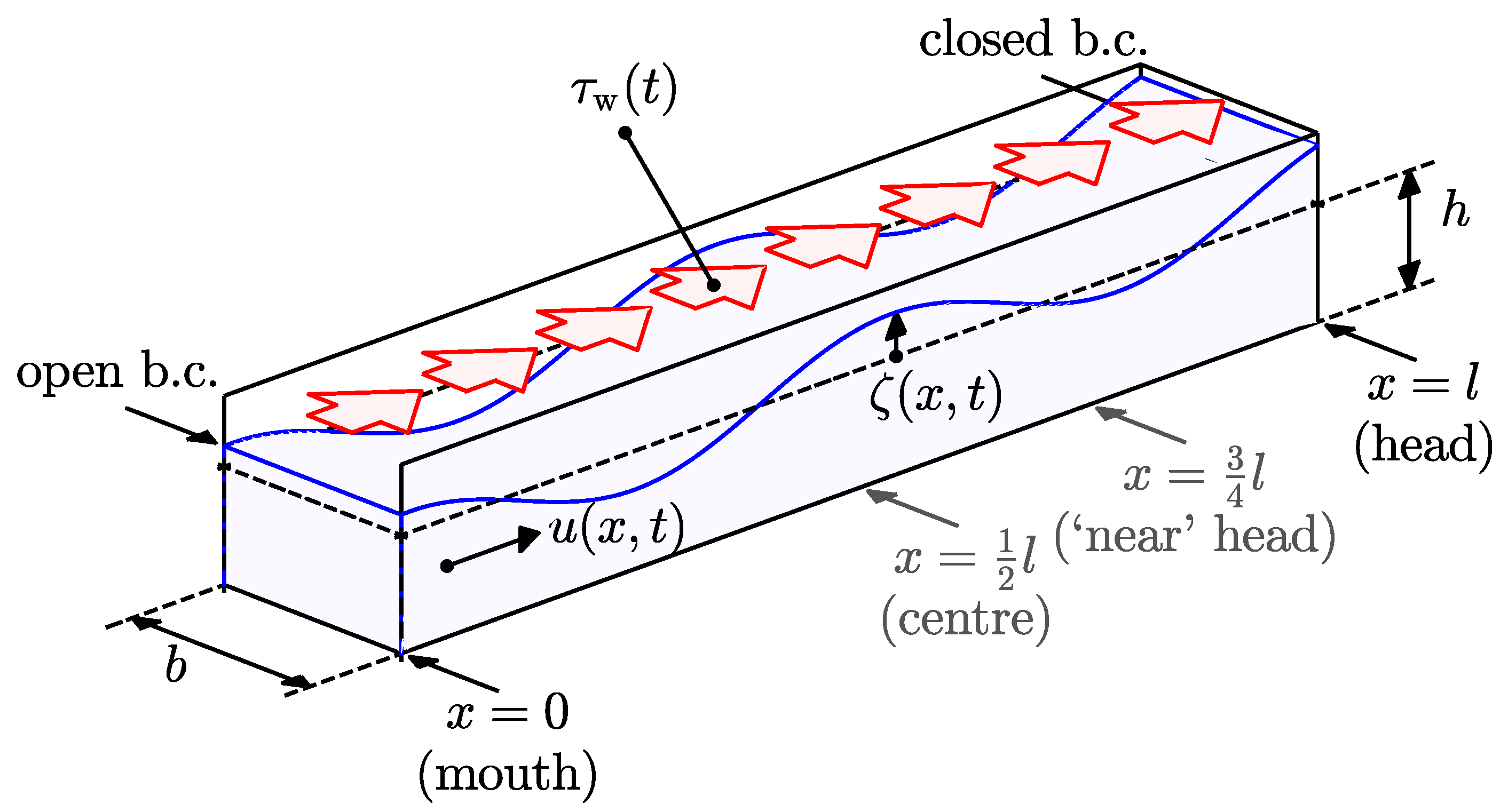
Consider a one-dimensional rectangular channel of length l, uniform width b and uniform undisturbed depth h (Figure 2). With x representing the along-channel coordinate, the channel has an open boundary at x = 0 , the ‘mouth’, and a closed boundary at x = l , the ‘head’. Let ζ ( x , t ) and u ( x , t ) denote the width-averaged free-surface elevation and the cross-sectionally averaged flow velocity, respectively, both defined as a function of the along-channel coordinate x and time t. Positive velocities are directed towards the channel head.
Assuming that | ζ | h b and adopting the linearisation posed by Equations (1) and (3), the cross-sectionally averaged mass and momentum balances in linearised form become
ζ t + h u x = 0 ,
u t + r ( t ) u h = g ζ x + τ w ( t ) ρ h .
Here, g is the gravitational acceleration, ρ is the water density, and τ w ( t ) is the along-channel component of the wind stress vector, which is time-dependent yet spatially uniform. The wind stress signal either comes from observed wind speeds (Figure 1) or represents a synthetic storm (Figure 3). It is treated as an external forcing term, implying that we do not account for the potential feedback of the water surface on the wind drag. The spatial uniformity of τ w is justified if the size of the channel is much smaller than the spatial scales of the atmospheric forcing such as, e.g., in the Wadden Sea; see [6]. In the notation of Equation (5), we emphasised the time-dependencies of the friction coefficient and the wind stress. Our time-varying wind stress suffices to represent an episodic and irregular external forcing, so we neglect atmospheric pressure gradients (but they could be readily added). Since this study concentrates on the bed shear stress, all other sources of nonlinearity (advective terms, contribution of the free-surface elevation to the water depth in the continuity and friction terms) were ignored from the outset.
The boundary conditions
ζ ( 0 , t ) = f ( t ) , u ( l , t ) = 0 ,
prescribe a surface elevation signal f ( t ) at the channel mouth and zero velocity at the channel head. As the initial conditions ( t = 0 ), we require either still water conditions or conditions in dynamic equilibrium with a tidal elevation signal at the channel mouth.
Finally, a novel friction coefficient r ( t ) is specified by equating the instantaneous power dissipated by both parametrisations in Equation (1), integrated over the entire channel:
r ( t ) = c d 0 l | u ( x , t ) | u ( x , t ) 2 d x 0 l u ( x , t ) 2 d x ( for   storm   surges ) .
Here, having performed spatial integration, we address the first caveat on equivalent linearisations in Section 1.
Importantly, the closure relationship in Equation (7) is the instantaneous (hence unsteady) counterpart of Lorentz’s classical linearisation with steady r if the latter is applied non-locally, so including spatial integration. The corresponding linearisation à la Lorentz is thus given by
r = c d 0 T 0 l | u ( x , t ) | u ( x , t ) 2 d x d t 0 T 0 l u ( x , t ) 2 d x d t ( for   tidal   flows ) .
Equation (8) reduces to Lorentz’s expression r = 8 3 π c d U of Equation (2) for the simple case of a spatially uniform and monochromatic flow velocity signal u ( x , t ) = U cos ω t with angular frequency ω = 2 π / T and velocity amplitude U.

3. Solution Procedure

3.1. Model Development

Eliminating the flow velocity from Equations (4)–(6) gives a damped wave equation for the surface elevation, supplemented with nonhomogeneous boundary conditions:
2 ζ t 2 + r ( t ) h ζ t g h 2 ζ x 2 = 0 , ζ ( 0 , t ) = f ( t ) , ζ x ( l , t ) = w ( t ) ,
where we introduced the dimensionless wind forcing w ( t ) = τ w ( t ) / ( ρ g h ) . To arrive at Equation (9), we first subtracted the space derivative of the momentum equation (multiplied by h) from the time derivative of the mass balance, and then used the mass balance again to express the friction term in ζ . Here, it is essential that both r ( t ) and τ w ( t ) do not depend on x. The boundary condition at x = l follows from inserting u ( l , t ) = 0 in the momentum equation. The problem in Equation (9) is linear in the unknown ζ and subject to two time-dependent forcing terms: the dimensionless wind forcing w ( t ) and the free-surface elevation at the channel mouth, f ( t ) .
Alternatively, by eliminating ζ instead of u, one could also solve the problem in terms of the flow velocity u. In either case, the other quantity ( ζ or u) will follow from applying one of the model equations.

3.2. Fourier Expansion

The governing equations in Equation (9) are solved in the frequency domain, leaning on the work by Chen et al. [14,15]. To this end, we expand all time-dependent variables in a discrete Fourier series according to
w ( t ) f ( t ) r ( t ) ζ ( x , t ) u ( x , t ) = m = M M W m F m R m Z m ( x ) U m ( x ) exp ( i ω m t ) , ω m = m ω 1 ,
with truncation number M and angular frequency ω m . For each mode m, we introduce complex Fourier components ( W m , F m , R m , Z m ( x ) , U m ( x ) ) of the wind forcing, boundary elevation, friction coefficient, surface elevation and flow velocity, respectively. Importantly, the last two are functions of the along-channel coordinate x; they will be expressed as sums of analytical expressions. Since all physical quantities are real-valued, it follows that W m = W m ¯ , F m = F m ¯ , etc., with an overbar denoting complex conjugation.
The discrete Fourier series in Equation (10) implies that both forcing and response are actually periodic over a time span T simul = 2 π / ω 1 associated with the lowest frequency ω 1 . By construction, the solution obtained here is directly in dynamic equilibrium with the periodic forcing; the transient propagation across the domain is not simulated. Choosing T simul sufficiently large, here in the order of 10 days (Figure 3), prevents interference among subsequent storm events and ensures that the initial conditions of Section 2 are indeed satisfied.

3.3. Iterative Procedure

The problem is now solved following an iterative procedure consisting of six steps:
  • Define an initial function of the friction coefficient r ( t ) = r init , e.g., zero or some other constant function, and determine the associated Fourier coefficients R m .
  • Find the surface elevation ζ ( x , t ) by solving Equation (9) in Fourier space. Since r ( t ) and R m are known, this problem is linear in the unknown complex amplitude functions Z m ( x ) . We solve it using matrix algebra (details in Appendix A.1).
  • Obtain the flow velocity u ( x , t ) by applying Equation (5). This provides the Fourier coefficients U m ( x ) (see Appendix A.2).
  • Substitute u ( x , t ) in Equation (7) to obtain an updated friction coefficient r ^ ( t ) . The integrals therein are evaluated on an equidistant grid with N points in the x-direction, using the trapezoidal rule. This step also produces new Fourier coefficients R ^ m .
  • Verify whether R ^ m and R m satisfy the convergence criterion
    1 T simul 0 T simul r ^ ( t ) r ( t ) 2 d t = m = M M | R ^ m R m | 2 < ϵ 2 ,
    with user-defined convergence tolerance ϵ . If so, the instantaneous power criterion is satisfied with sufficient precision over the entire simulation time, the current solution is converged in the sense of the second caveat on equivalent linearisations in Section 1, and the procedure is completed.
  • If Equation (11) is not satisfied, apply relaxation to find the next guess for the friction coefficient: r new ( t ) = α r ^ ( t ) + ( 1 α ) r ( t ) , with a relaxation parameter α that can be tuned to accelerate convergence. Then, repeat the procedure from step 2 onward using the new function r ( t ) = r new ( t ) and the associated Fourier coefficients R m = R new , m .
The truncation number M, simulation period T simul , number N of spatial points used in the numerical integration of Equation (7), relaxation parameter α and convergence tolerance ϵ are the user-defined parameters of our solution method: see Table 1 and Discussion in Section 5.

3.4. Procedure for the Steady Friction Coefficient

As mentioned in Section 1, we conducted simulations with a steady friction coefficient r for the purpose of comparison. Such a steady r-value is implemented by applying steps 1–3 of the procedure in Section 3.3 once. Unlike Lorentz’s original procedure, this formulation is not solely tidal and the steady r-value can be arbitrary, not necessarily tied to an energy criterion.

3.5. Reference Finite-Difference Solution with Quadratic Bed Shear Stress

A finite-difference solution with the conventional quadratic parametrisation of the bed shear stress was used to evaluate the goodness of the linear parametrisations with r and r ( t ) . To this end, we solved Equations (4) and (5) after replacing the bottom friction term r ( t ) u / h with c d | u | u / h , recalling Equation (1).
We used a staggered uniform grid with spacing Δ x and time step Δ t , consisting of elevation and velocity points that, relative to one another, were shifted over half a step in both space and time. In view of the boundary conditions in Equation (6), the grid was chosen such that x = 0 coincided with an elevation point, and x = l with a velocity point. We then applied a leap-frog scheme—i.e., central discretisations of the derivatives in Equations (4) and (5) evaluated at staggered points in space and time—and iteratively computed the velocity in the quadratic bottom friction term. The discretisation adopted is second-order accurate in space and time.
The initial conditions prescribe still water. Importantly, these conditions actually serve as a ‘cold start’ for the simulations with tidal fluctuations at the channel head. The model spins up for a first T simul -long span (see Figure 3) to simulate the transient and produces the desired solution in dynamic equilibrium with the periodic forcing in the second T simul -long span. This treatment enables a proper comparison with the Fourier solution, since in Section 3.2 we chose T simul sufficiently long to fulfil this purpose.
The grid spacing and time step (Table 1) are such that the numerical solution is stable and sufficiently converged. Furthermore, the shortest oscillations resolved by the finite-difference solution ( T min FD = 2 Δ t = 120 s ) are much shorter than those associated with the highest frequency of the Fourier expansion (10) in our new model ( T min Four = T simul / M = 1687.5 s ). Therefore, the finite-difference solution is indeed a trustworthy benchmark for the comparisons presented in Section 4.

4. Results

4.1. Wind Forcing Only: Synthetic Storm Event

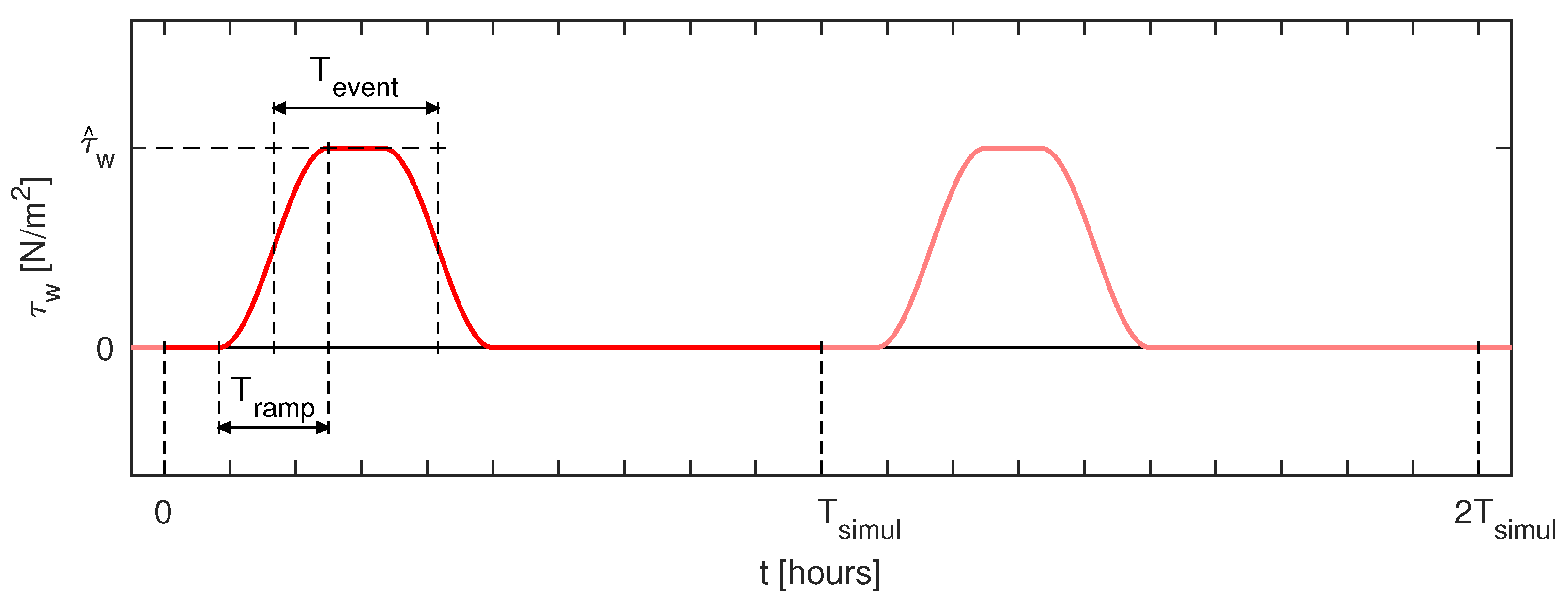
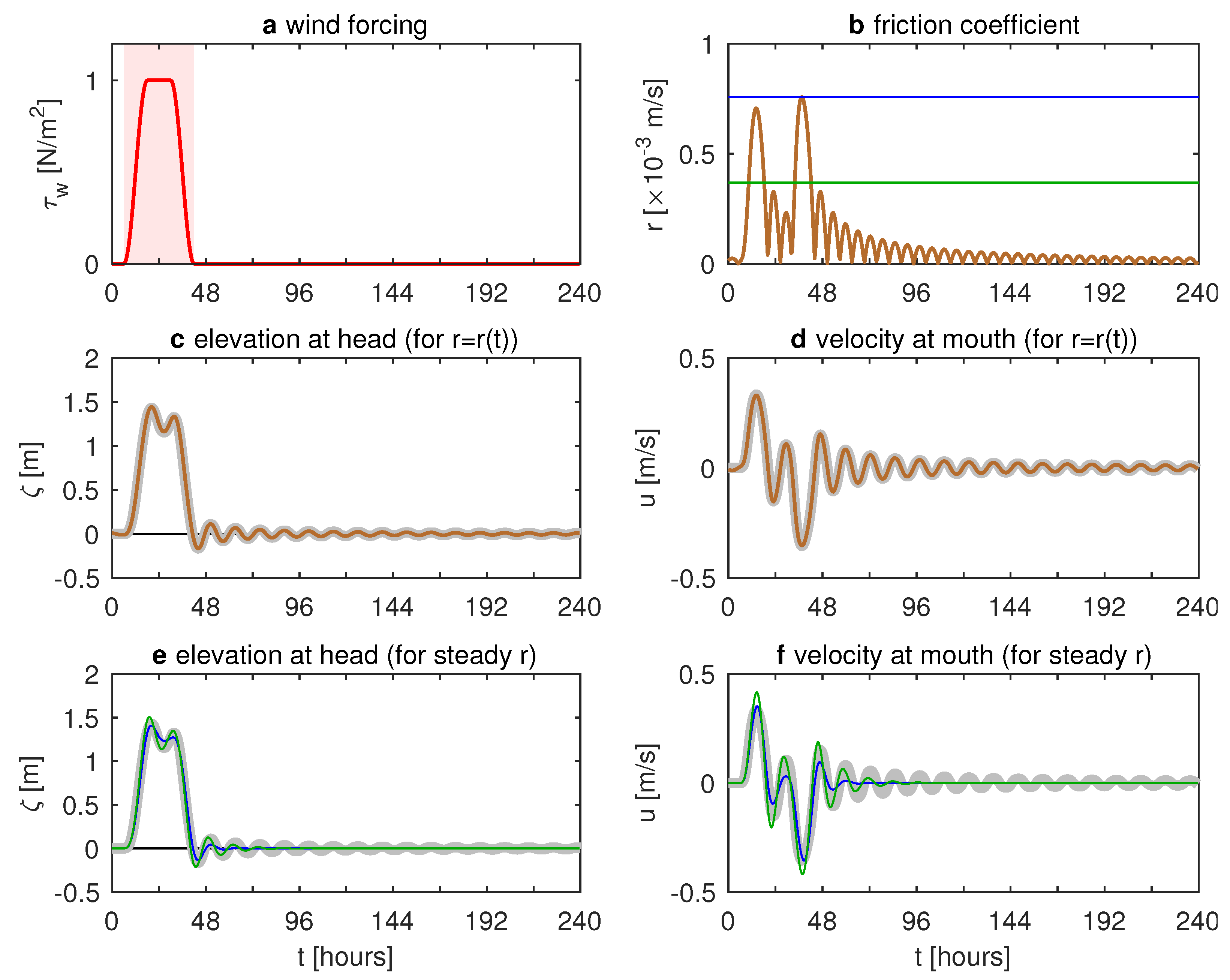
First off, we tested the new model for the case of wind forcing only (Figure 4). Our reference channel (100 km long, 8 m deep, see Table 1) is subject to the synthetic wind stress signal as defined in Figure 3, with a peak value of τ ^ w = 1 N m 2 , a duration T event = 24 h and a ramp-up time T ramp = 12 h . The total simulation time is 10 days (Figure 4a). An a priori scale analysis (Appendix B) shows that, for these parameter values, bottom friction is of first order importance.
The iterative procedure converges to an unsteady friction coefficient r ( t ) (Figure 4b), displaying pronounced peaks during ramp-up and ramp-down, as well as decaying oscillations at the tail of the stormThese oscillations are associated with the sloshing motion evident from both the elevation at the channel head (Figure 4c) and the velocity at the channel mouth (Figure 4d).
The results with the unsteady friction coefficient show excellent agreement with the reference solution retaining the quadratic bed shear stress (shown by the grey lines in Figure 4c,d). In contrast, such agreement breaks down for the two examples with steady friction also shown: one with the maximum value r max and one with the mean value r mean (averaged over the time span of T event + T ramp = 36 h with nonzero wind stress, shaded in pink in Figure 4a). The case with strong steady friction ( r = r max ) suppresses the sloshing of the surface elevation at the channel head and produces a deformed elevation curve underestimating and delaying the peak surge. Alternatively, the milder friction case ( r = r mean ) produces an early overestimated peak, a single undershoot after the event and no trailing oscillations. The same shortcomings occur in the velocity signal at the channel head (Figure 4f).
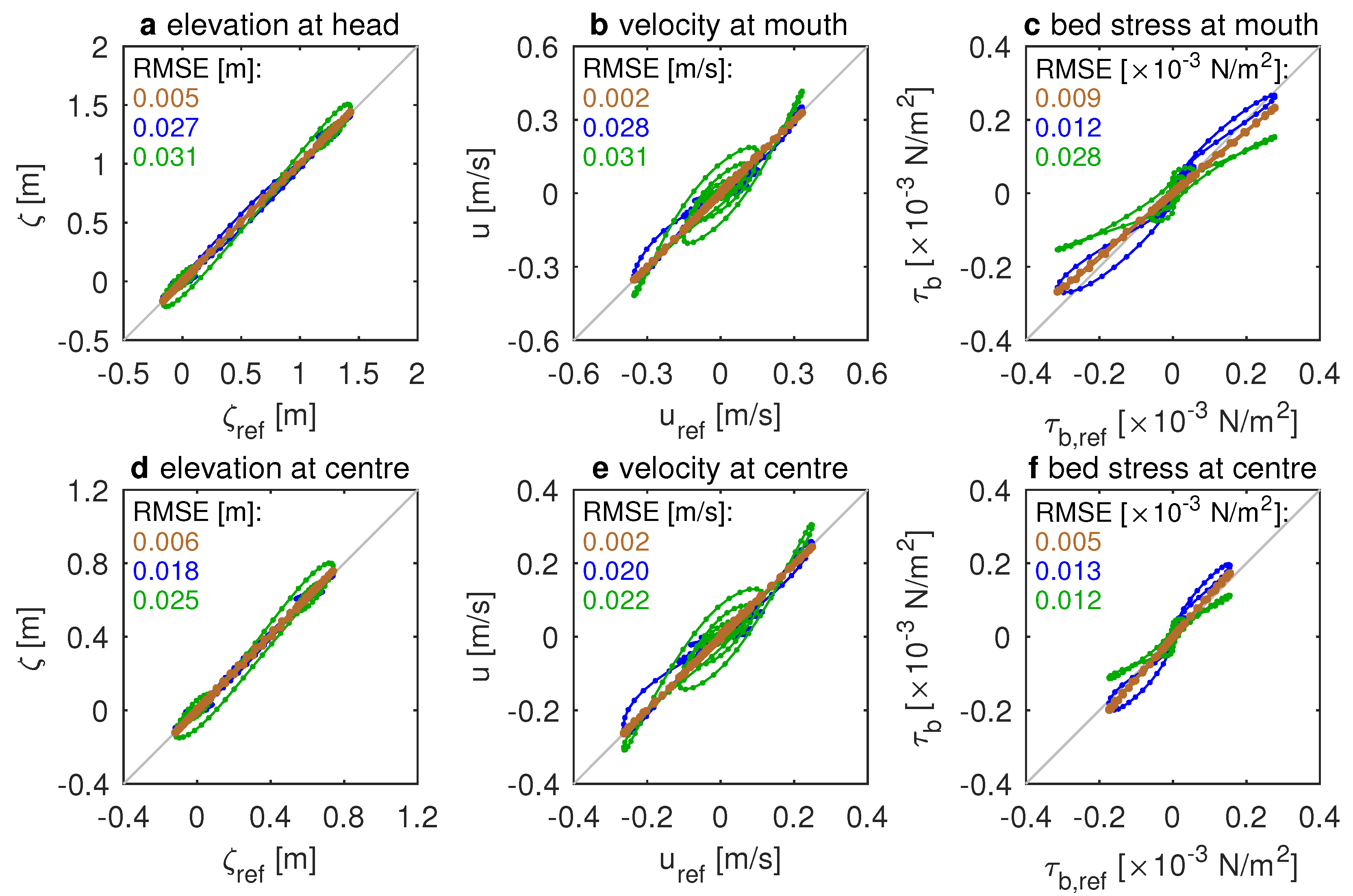
The scatter plots of Figure 5 contrast the results from all variants of the linear friction coefficient with the finite-difference quadratic reference. The bed shear stress at the channel mouth is also shown alongside the surface elevation at the head and the velocity at the mouth. The steady friction coefficients produce significantly poorer signals of those quantities than the unsteady formulation, regarding magnitude and/or phasing, which is confirmed by the RMSE-values in the insets. The same degree of goodness was also found at other locations in the channel (such as the centre, Figure 5d–f). Therefore, the new approach reproduces the flow solution caused by synthetic unsteady signals of the wind stress with great accuracy. Furthermore, the comparison with the reference solution confirms the merits of the unsteady linearisation of the friction coefficient over steady linearisations.

4.2. Wind and Tide Forcing

After the purely wind-driven flows, we addressed the tide-surge interactions induced by bottom stress. To this end, we considered the same channel geometry and the same synthetic wind stress signal τ w ( t ) as in Section 4.1 and Table 1, plus a tidal signal f ( t ) for the surface elevation at the channel mouth (Figure 6a). The latter is an S2-signal with an amplitude F ^ , given by
f ( t ) = F ^ cos ω tide t , ω tide = 2 π T tide .
Importantly, the total simulation period is an integer multiple of the tidal period, namely T simul = 20 T tide with T tide = 12 h .
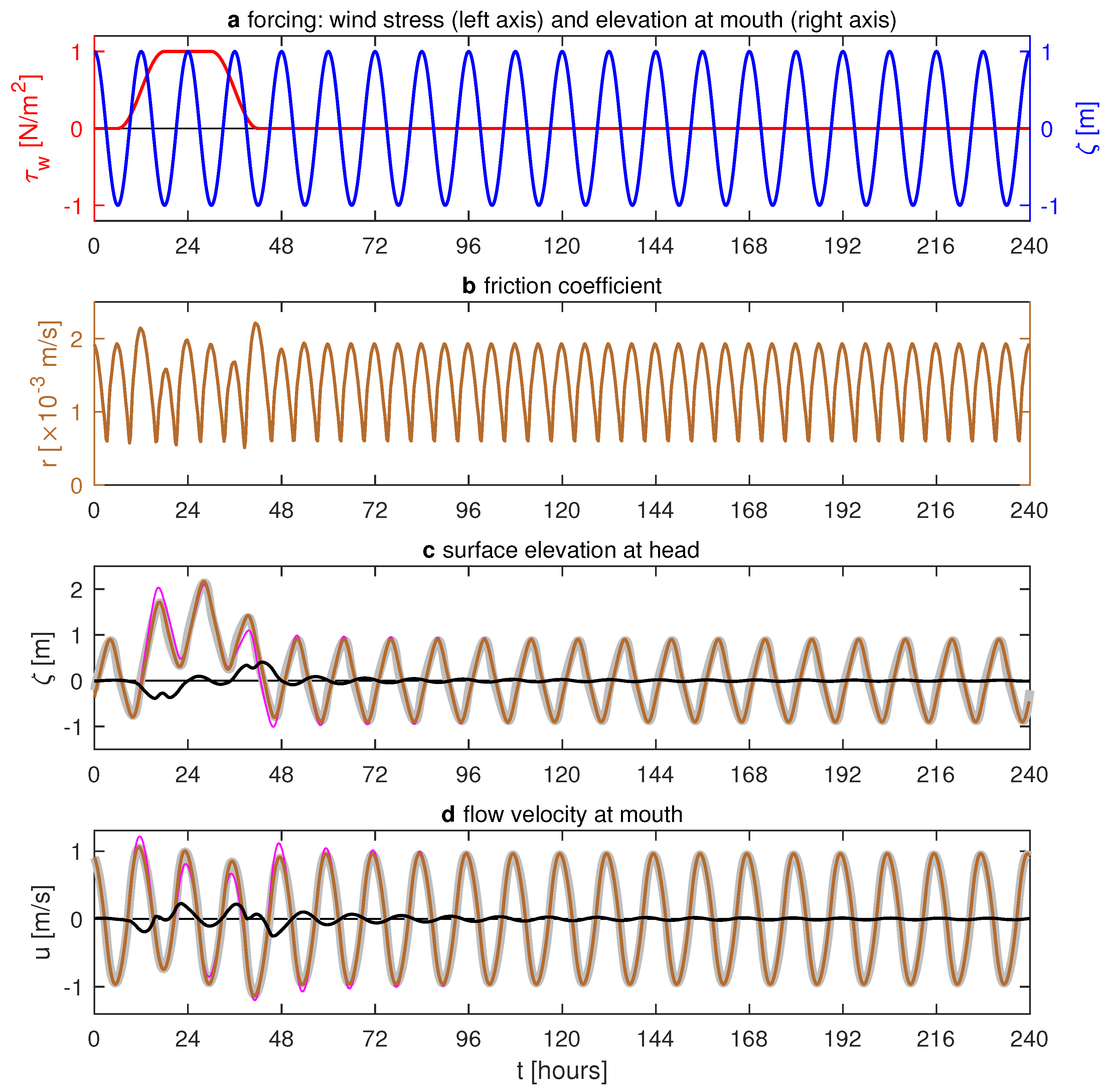
As anticipated in the objectives of Section 1, the unsteady friction coefficient is subject to tidal fluctuations distorted by interference with the storm event (Figure 6). Unlike the wind-only case, the friction coefficient does not decay to zero because of the background tidal flow (Figure 6b).
The surface elevation at the channel head contains friction-induced tide-surge interactions (Figure 6c), because the combined wind-tide solution (orange line) differs from the sum of the wind-only and tide-only solutions (thin pink line). We note the good agreement between our new model (orange line) and the reference finite-difference solution (grey line) over the entire simulation period. The tide-surge interaction subsequently produces negative differences, i.e., a set-down overhead, during the onset of the storm; then produces positive differences, i.e., a set-up overhead, during the fall of the storm (black line); and vanishes after the storm event as expected.

4.3. Realistic Wind Forcing

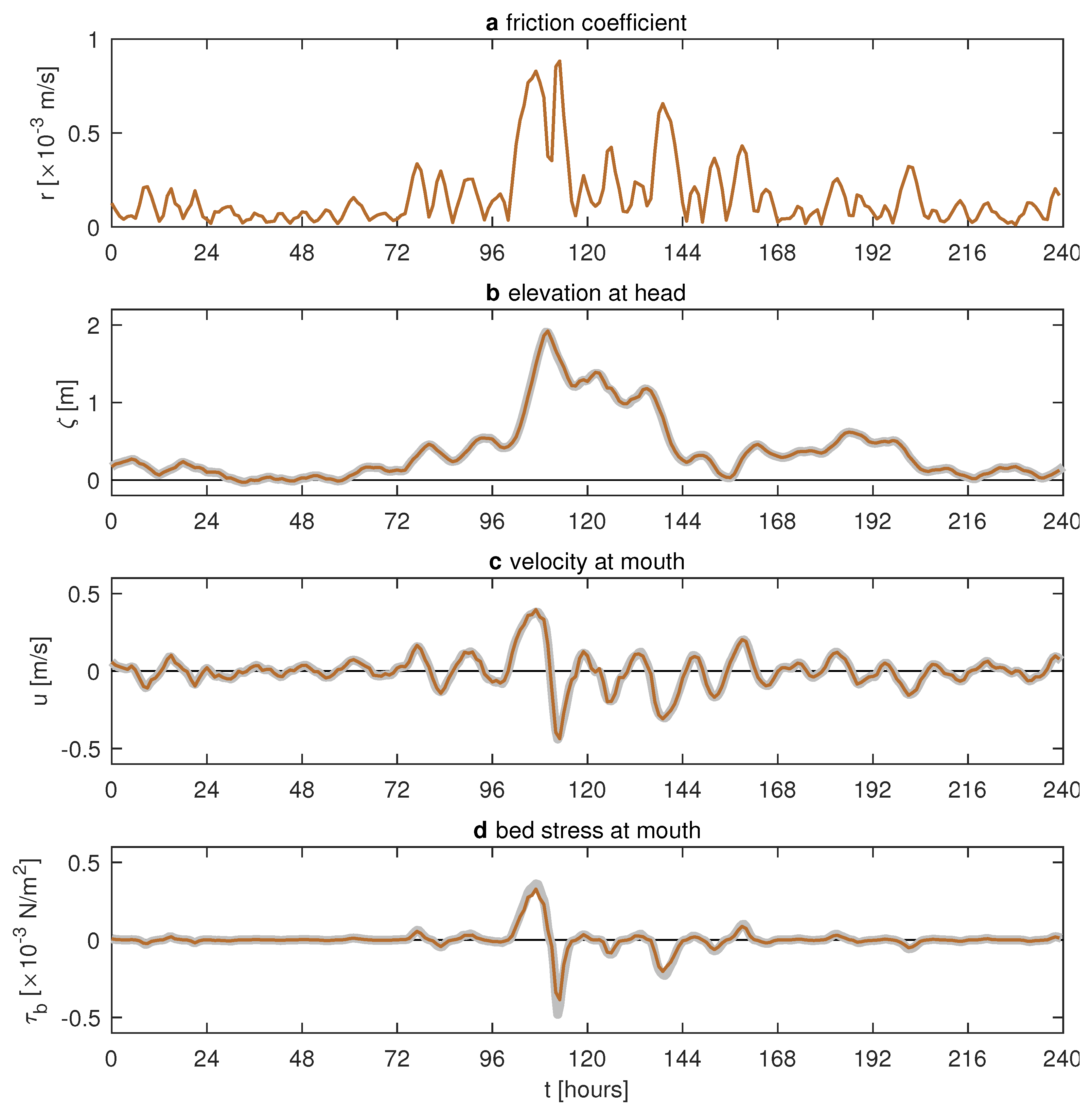
Finally, we address the modelling of realistic, unsteady and irregular signals of the wind stress. To this end, we considered the same channel as in Section 4.1 and Table 1 and applied the wind stress signal of the Xavier or Sinterklaas storm in the Wadden Sea (Figure 1). Excluding tides for simplicity, we set the surface elevation at the channel mouth to zero, i.e., f ( t ) = 0 in Equations (6) and (9).
In Figure 7, we compare the solution using the unsteady friction coefficient with the reference finite-difference solution. For the latter, as explained in Section 3.5, we imposed the periodic continuation of the wind stress signal in Figure 1 and simulated a period of 2 T simul = 480 h , using the first 240 h for the spin-up and the second 240 h for the model results. These show that the unsteady friction coefficient follows the natural evolution of the storm (Figure 7a); and that the agreement with the reference finite-difference solution is excellent for elevation, velocity and bed shear stress (Figure 7b–d). Therefore, the new approach is also capable of accurately handling the irregular and unsteady signals of real-world storms.

5. Discussion

Denominator of bottom friction term. The bed shear stress parametrisation obviously pertains to the numerator of the bottom friction term in Equation (5). For the denominator, we assumed that h + ζ h and thus relied on small values of | ζ | / h . The peak water levels in the storm surge simulations presented in Section 4 are characterised by | ζ | / h 0.25 and this ratio is expected to increase for surges in shallower channels. Further research will address the significance and validity of the above approximation in the friction term for channels of arbitrary depth.
Power criterion. The unsteady linearisation of the bed shear stress circumvents the problem of finding an appropriate velocity scale for situations with episodic and irregular forcings, cf. U in Equation (2). In fact, this aspect is covered by the power criterion in Equation (7) and thus anchored in that physical statement. Not only do steady friction coefficients produce inaccurate wind-driven simulations (Section 4.1), but they are also arbitrary due to the lack of a physically sound basis. For example, why choose precisely r = r max [16]? Or, when opting for a time-averaged value r = r mean , over what time span should one average? The choice of this time span should be independent of the artificial numerical parameter T simul .
Channel-wide bottom friction. An essential property of our approach is that the unsteady friction coefficient r ( t ) is spatially uniform, i.e., it is representative of the entire channel. This is guaranteed for solutions in which the flow velocities u ( x , t ) do not vary considerably over the domain. Otherwise, the spatial averaging in Equation (7) may imply a poor r ( t ) -estimate. One can test for and resolve this limitation by splitting the channel in several subchannels, each having an individual friction coefficient r j ( t ) . This segmentation is actually a special case of the channel network discussed below. Furthermore, a constant drag coefficient c d , which effectively turns the general nonlinear stress law into a purely quadratic one, is by no means restrictive. Equation (7) can be readily adjusted to incorporate any law for the dependency of c d on u and h.
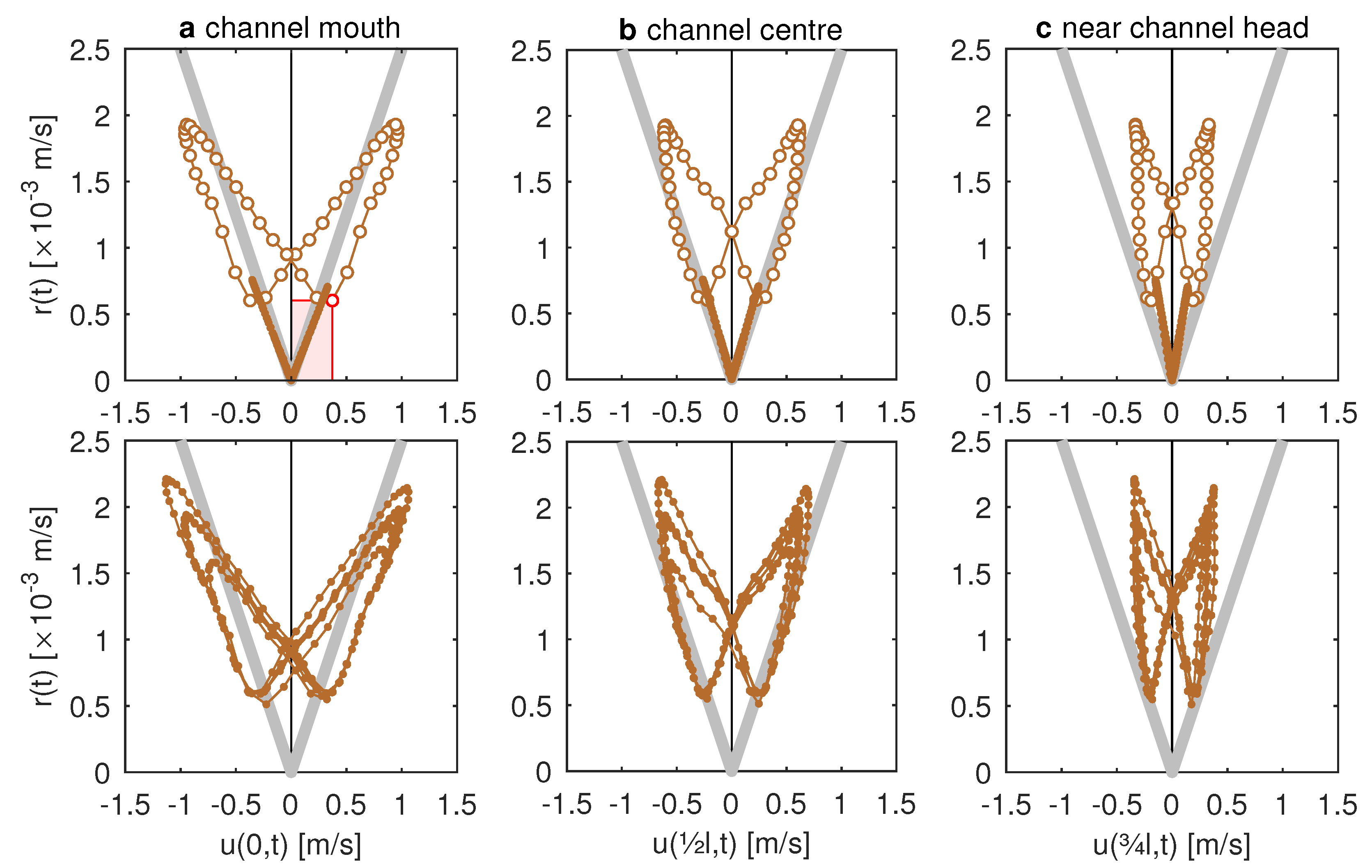
Interpretation of the unsteady friction coefficient. Given the r ( t ) -signals shown in Figure 4b, Figure 6b and Figure 7a, we also inspect how the channel-wide unsteady friction coefficient relates to local and instantaneous flow velocities. To this end, Figure 8 shows the scatter plots of r ( t ) versus u ( x ^ , t ) at the channel mouth, the channel centre and near the channel head, with each data point representing a time instant in a simulation. By construction, the magnitude of the instantaneous bed stress is proportional to the area of the rectangle having that point and the origin as opposite corners (see pink-shaded example). The grey V-shaped lines draw the values r = c d | u | for which, recalling the bed stress parametrisation in Equation (1), the channel-wide linear formulation coincides with the local quadratic one. Please take note that this comparison is not a model verification, which was performed in Section 4 on the basis of time series of elevation, flow velocity, and bed stress. We carried out this analysis for the wind-only, tide-only, and combined wind-tide simulations presented in Section 4.1 and Section 4.2:
  • For the wind-only simulations, r ( t ) closely follows the quadratic parametrisation, as shown by the V-shaped arrangement of the data points in the top of Figure 8;
  • For the tide-only simulations, r ( t ) follows an oscillatory path and the continuous presence of nonzero currents inside the channel prevents it from approaching zero;
  • Finally, for wind-tide simulations, the path of r ( t ) -values is similar to the combined path for wind and tide forcing but is additionally deformed by the tide-surge interactions.
Solution procedure and numerical settings. Our solution method in the frequency domain enables us to combine analytical solutions (Appendix A) in a way that is analogous to the classical approach with steady friction. The numerical parameters should be chosen with care. For example, as a consequence of imposing periodic solutions, the simulation period T simul should be large enough to prevent the interference of subsequent events (as depicted in Figure 3). Furthermore, the truncation number M should be so large that the shortest fluctuations in the forcing and the solution, T simul / M are resolved with sufficient accuracy. Finally, the iterative procedure appeared to be equally robust for the unsteady and steady friction coefficients. In all simulations carried out, it converged to a unique function r ( t ) , independent of the relaxation parameter α and the initial value r init (see Section 3.3 and Table 1). The iterative procedure accounts for the dependency of r ( t ) on u ( x , t ) according to Equation (7) and emphasises the nonlinearity still present in the model (recall the second caveat on equivalent linearisations in Section 1).
Extension to channel network. The application of an unsteady friction coefficient to a single channel can be readily extended to a network of channels, as performed earlier for tides and storm surges—both separately [6] and jointly [16]. To this end, one should account for the orientation of subchannels with respect to wind direction. Furthermore, one must specify appropriate matching conditions at the internal nodes where subchannels meet (continuity of elevation and discharge) and boundary conditions at the terminal nodes (open or closed). The iterative procedure presented in Section 3 then concerns the friction coefficients r j ( t ) of the entire network. The extension to a channel network, implemented and tested by Pitzalis [17], is beyond the scope of the present study.

6. Conclusions

We devised and tested a novel time-dependent linearisation of bed shear stress extending Lorentz’s classical linearisation to the idealised modelling of storm surges in (tidal) channels. This approach consists of two elements: (i) the formulation of an instantaneous power equivalence criterion to specify an unsteady channel-averaged friction coefficient r ( t ) ; and (ii) a straightforward iterative procedure, carried out in the frequency domain, to obtain both r ( t ) and the corresponding solution of the linearised shallow-water equations. By construction, the unsteady friction coefficient r ( t ) adjusts to the intensity of the flow inside the domain. Qualitatively, r ( t ) is large whenever the flow is strong and small when it is weak. As a result, we circumvent the issue of specifying a single velocity scale for the bottom friction term during episodic and irregular wind forcing.
The verification with a reference solution in the time domain retaining the quadratic bed shear stress shows excellent agreement throughout the channel in the time series of elevation, flow velocity, and bed shear. Distinctive aspects of the surge dynamics influenced by bed shear stress, such as the timing and magnitude of peaks, sloshing motions and tide-surge interactions, are well captured qualitatively and quantitatively. This conclusion holds for both synthetic and realistic wind forcings. In contrast, steady friction coefficients fail to produce such an agreement.
The unsteady linearisation of bed stress has led to a process-based idealised model that is amenable for extensive sensitivity analyses of storm surges. The model produces time series of bed shear stress throughout the channel, which indicates a potential application in morphodynamics, e.g., in terms of event-averaged bed evolution.

Author Contributions

Conceptualisation, P.C.R.; methodology, P.C.R., G.L., C.P., K.R.G.R. and G.H.P.C.; software, C.P. and G.H.P.C.; validation, P.C.R., G.L. and C.P.; formal analysis, P.C.R., G.L. and C.P.; investigation, C.P.; writing—original draft preparation, P.C.R.; writing—review and editing, P.C.R., G.L., C.P., K.R.G.R., G.H.P.C. and S.J.M.H.H.; visualisation, P.C.R. and G.L.; supervision, S.J.M.H.H.; project administration, C.P.; funding acquisition, S.J.M.H.H. All authors have read and agreed to the published version of the manuscript.

Funding

This research was carried out within the WADSnext! project, co-funded by the ‘Simon Stevin Meester’ prize (awarded by the Dutch Research Council NWO to S.J.M.H.H. in 2016).

Data Availability Statement

The data underlying this study are available upon request.

Conflicts of Interest

The authors declare no conflict of interest.

Appendix A. Details of the Solution Procedure

Appendix A.1. Step 1: Surface Elevation

In the frequency domain, i.e., for the m-th Fourier mode, the problem posed by Equation (9) transforms into a set of coupled Helmholtz problems for the complex amplitude functions Z m ( x ) (for m = M , , M ):
Z m 1 g h ( i ω m ) 2 Z m + 1 h n = n 1 n 2 R m n i ω n Z n = 0 , Z m ( 0 ) = F m , Z m ( l ) = W m ,
with summation bounds n 1 = M + max { 0 , m } and n 2 = M + min { 0 , m } and primes indicating differentiation with respect to x. The last term on the left-hand side of the differential equation is a convolution sum, expressing the mode interaction due to the unsteady friction coefficient. In matrix notation, Equation (A1) reads
z + A z = 0 , z ( 0 ) = f , z ( l ) = w ,
with the ( 2 M + 1 ) × ( 2 M + 1 ) -matrix A = 1 g h T + 1 h R T which generally contains nonzero off-diagonal elements. The problem in Equation (A2) is solved by matrix diagonalisation. To this end, let P be such that D = P 1 A P is diagonal, with the eigenvalues ( μ M 2 , , μ 0 2 , , μ M 2 ) as diagonal elements. Introducing a new unknown
z ˜ = P 1 z ,
the coupled problem in Equation (A2) then transforms into an uncoupled problem for z ˜ . This problem, uncoupled due to D ’s diagonality, is given by
z ˜ + D z ˜ = 0 , z ˜ ( 0 ) = f ˜ , z ˜ ( l ) = w ˜ ,
where f ˜ = P 1 f and w ˜ = P 1 w are transformed forcing terms with elements F ˜ m and W ˜ m , respectively. The analytical solution to Equation (A4) is given by
Z ˜ m ( x ) = F ˜ m cos μ m x + F ˜ m tan μ m l + W ˜ m μ m cos μ m l sin μ m x if   μ m 0 , F ˜ m + W ˜ m x if   μ m = 0 ,
for m = M , , M . Using the inverse of Equation (A3), we then transform back to find the components Z m ( x ) of z . This also gives the Fourier components Z m ( x ) of the surface slope z .

Appendix A.2. Step 2: Flow Velocity

In the frequency domain, the momentum equation, as given by Equation (5), is written as
T + 1 h R u = g z w .
In any case, it follows from the continuity equation and the closed boundary condition at x = l that U 0 ( x ) = 0 for all x. The other components, i.e., U m ( x ) for nonzero m depends on friction. For nonzero friction ( r ( t ) 0 and in particular R 0 0 ), the above matrix equation is readily solved to find all U m ( x ) . Without friction ( r ( t ) 0 ), one directly finds U m = g [ Z m ( x ) W m ] / ( i ω m ) for m 0 .

Appendix B. Scaling Analysis

Before performing the model simulations for the chosen parameter values, it is necessary to ascertain whether in the momentum equation, the magnitude of the bottom friction term is at least comparable to that of the inertia term. Using square brackets to denote magnitudes, it follows from Equation (5) that
u t U ^ T ramp , c d | u | u h c d U ^ 2 h ,
whereby the ratio of the bottom friction and the inertia scales is given by
β = c d | u | u h / u t c d T ramp U ^ h .
The parameter values in this expression are known from Table 1, except for the velocity scale U ^ . To estimate U ^ , we assume a balance between either (i) inertia and wind stress or (ii) bottom friction and wind stress (requiring the other terms to be smaller in both cases). With the magnitude of the wind stress term given by τ w / ( ρ h ) τ ^ w / ( ρ h ) , we thus obtain
U ^ ( i ) = τ ^ w T ramp ρ h = 5.4 m s 1 , U ^ ( ii ) = τ ^ w c d ρ = 0.63 m s 1 ,
respectively. The first velocity scale, U ^ ( i ) , is unphysical, because it would render the friction term so large that it cannot be balanced by any of the other terms. We thus adopt the second, U ^ ( ii ) , for which the ratio in Equation (A8) becomes
β = T ramp h c d τ ^ w ρ = 8.5 = O ( 10 ) .
We conclude that, for the simulations carried out in this study, bottom friction is indeed of first order importance in the governing equations.

References

  1. Pugh, D.T.; Woodworth, P.L. Sea-Level Science. Understanding Tides, Surges, Tsunamis and Mean Sea-Level Changes; Cambridge University Press: Cambridge, UK, 2014. [Google Scholar]
  2. Prandle, D.; Wolf, J. The interaction of surge and tide in the North Sea and River Thames. Geophys. J. R. Astr. Soc. 1978, 55, 203–216. [Google Scholar] [CrossRef] [Green Version]
  3. Horsburgh, K.J.; Wilson, C. Tide-surge interaction and its role in the distribution of surge residuals in the North Sea. J. Geophys. Res. 2007, 112, C08003. [Google Scholar] [CrossRef] [Green Version]
  4. Murray, A.B. Contrasting the goals, strategies, and predictions associated with simplified numerical models and detailed simulations. In Predictions in Geomorphology; Geophysical, M., Iverson, R.M., Wilcock, P.R., Eds.; AGU: Washington, DC, USA, 2003; Volume 135, pp. 151–165. [Google Scholar]
  5. Lorentz, H.A. Het in rekening brengen van den weerstand bij schommelende vloeistofbewegingen. De Ingenieur 1922, 37, 695. [Google Scholar]
  6. Lorentz, H.A. Verslag van de Staatscommissie Zuiderzee 1918–1926; Technical Report; Algemeene Landsdrukkerij: Den Haag, The Netherlands, 1926. [Google Scholar]
  7. Mei, C.C. The Applied Dynamics of Ocean Surface Waves; World Scientific: Singapore, 1989. [Google Scholar]
  8. Zimmerman, J.T.F. On the Lorentz linearization of a nonlinearly damped tidal Helmholtz oscillator. Proc. Kon. Ned. Akad. v. Wetensch. 1992, 95, 127–145. [Google Scholar]
  9. Roos, P.C.; Velema, J.J.; Hulscher, S.J.M.H.; Stolk, A. An idealized model of tidal dynamics in the North Sea: Resonance properties and response to large-scale changes. Ocean Dyn. 2011, 61, 2019–2035. [Google Scholar] [CrossRef] [Green Version]
  10. Hulscher, S.J.M.H.; de Swart, H.E.; de Vriend, H.J. The generation of offshore tidal sand banks and sand waves. Cont. Shelf Res. 1993, 13, 1183–1204. [Google Scholar] [CrossRef] [Green Version]
  11. Terra, G.M.; van de Berg, W.J.; Maas, L.R.M. Experimental verification of Lorentz’ linearization procedure for quadratic friction. Fluid Dyn. Res. 2005, 36, 175–188. [Google Scholar] [CrossRef] [Green Version]
  12. Jeffreys, H. The Earth: Its Origin, History and Physical Constitution, 5th ed.; Cambridge University Press: Cambridge, UK, 1970. [Google Scholar]
  13. Inoue, R.; Garrett, C. Fourier Representation of Quadratic Friction. J. Phys. Oceanogr. 2007, 37, 593–610. [Google Scholar] [CrossRef]
  14. Chen, W.L.; Roos, P.C.; Schuttelaars, H.M.; Hulscher, S.J.M.H. Resonance properties of a closed rotating rectangular basin subject to space- and time-dependent wind forcing. Ocean Dyn. 2015, 65, 325–339. [Google Scholar] [CrossRef] [Green Version]
  15. Chen, W.L.; Roos, P.C.; Schuttelaars, H.M.; Kumar, M.; Zitman, T.J.; Hulscher, S.J.M.H. Response of large-scale coastal basins to wind forcing: Influence of topography. Ocean Dyn. 2016, 66, 549–565. [Google Scholar] [CrossRef] [Green Version]
  16. Reef, K.R.G.; Lipari, G.; Roos, P.C.; Hulscher, S.J.M.H. Time-varying storm surges on Lorentz’s Wadden Sea networks. Ocean Dyn. 2018, 68, 1051–1065. [Google Scholar] [CrossRef] [Green Version]
  17. Pitzalis, C. Time-Dependent Linearized Friction: A Development on Lorentz’ Energy Argument. Master’s Thesis, Civil Engineering & Management, University of Twente, Enschede, The Netherlands, 2017. [Google Scholar]
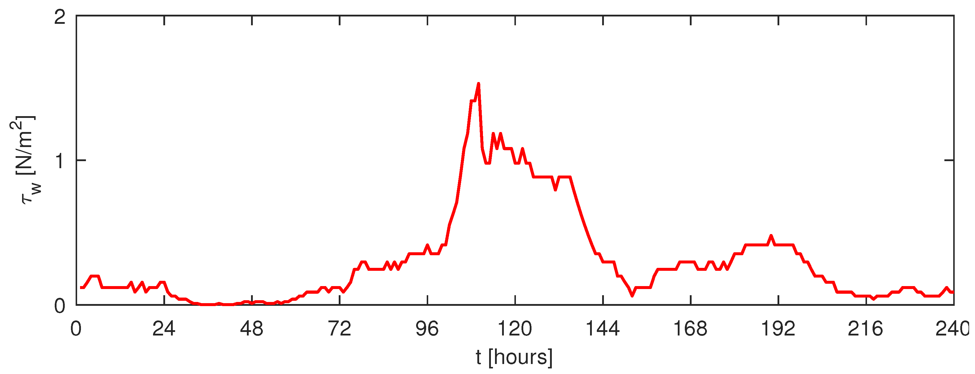
Figure 1. Time series of the wind stress τ w ( t ) during the Xavier or Sinterklaas storm in the Wadden Sea (peak values on 5 December 2013; t = 0 corresponds to 1-12-2013 00:00 CET). Wind speed data at the Vlieland station of the Royal Netherlands Meteorological Institute (KNMI). Stress law τ w = ρ air c w | u w | u w with air density ρ air = 1.225 kg m 3 and wind drag coefficient c w = 2 × 10 3 , e.g., [1].
Jmse 09 01160 g001
Figure 2. Model geometry showing the rectangular channel with one open and one closed end, subject to time-dependent signals of wind stress, τ w ( t ) , and surface elevation at the open boundary. The arrows used to denote the flow velocity u, surface elevation ζ and wind stress point in the direction where these quantities are positive. Apart from at the mouth and head, we also present model results at two intermediate positions: the channel centre and ‘near’ the head.
Jmse 09 01160 g002
Figure 3. Synthetic wind forcing τ w ( t ) , describing a storm event of duration T event , with peak amplitude τ ^ w and a sinusoidal ramp-up stage of duration T ramp (same duration as ramp-down stage). As implied by our solution method (Section 3), the forcing is periodic over a time span T simul . Parameter values in Table 1. N.B.: T event is defined such that the time-integrated wind stress equals τ ^ w T event , i.e., independently of T ramp .
Jmse 09 01160 g003
Figure 4. Model results for wind forcing only: (a) synthetic wind stress signal (nonzero in the pink shaded window, zero outside it); (b) unsteady friction coefficient r ( t ) (brown) and its maximum (blue) and mean (green) values; (c,d) elevation at head and velocity at mouth for unsteady friction coefficient r ( t ) ; (e,f) same quantities, but now using maximum and mean values as steady friction coefficients r. In (cf), the thick grey lines represent the reference finite-difference solution. Parameter values are in Table 1.
Jmse 09 01160 g004
Figure 5. Scatter plots showing results with unsteady friction coefficient (vertical axis) versus the reference finite-difference solution (horizontal axis): (a) elevation at channel head; (b) velocity at mouth; (c) bed shear stress at mouth; (d) elevation at centre; (e) velocity at centre; and (f) bed shear stress at centre. Shown here are the cases with unsteady r ( t ) (brown) and those with steady coefficients r = r max (blue) and r = r mean (green). The coloured numbers indicate the corresponding RMSE-values.
Jmse 09 01160 g005
Figure 6. Model results for combined wind and tide forcing: (a) synthetic wind stress signal (red, left axis) and tidal surface elevation signal f ( t ) (blue, right axis); (b) unsteady friction coefficient r ( t ) ; (c) elevation at the channel head from different solutions: combined wind-tide solution (brown), superposition of the separate wind-only and tide-only solutions (pink), and the tide-surge interaction (black, equals brown minus pink). The thick grey line represents the reference finite-difference solution obtained for the combined problem; (d) same as c, but now for the velocity at the channel mouth.
Jmse 09 01160 g006
Figure 7. Model results for a single channel subject to the wind stress signal of the Xavier or Sinterklaas storm (plotted in Figure 1): (a) time-dependent bottom friction coefficient r ( t ) ; (b) elevation at the channel head; (c) velocity at mouth; and (d) bed stress at mouth. In (bd), the thick grey line represents the reference finite-difference solution.
Jmse 09 01160 g007
Figure 8. Scatter plots of the friction coefficient r ( t ) versus the flow velocity u ( x ^ , t ) for the model simulations in Section 4.1 and Section 4.2 at three locations: (a) channel mouth ( x ^ = 0 ); (b) channel centre ( x ^ = 1 2 l ); (c) near channel head ( x ^ = 3 4 l ). The top row shows the surge-only (dots) and tide-only (open circles) simulations, the bottom row the combined tide-surge simulations (dots). The magnitude of τ b ( x ^ , t ) / ρ equals the area of the rectangle with ( 0 , 0 ) and ( u ( x ^ , t ) , r ( t ) ) as opposite vertices: see the pink-shaded example in the top left plot. Grey lines indicate r ( t ) -values locally identical to a quadratic parametrisation of the bed shear stress. Parameter values are in Table 1.
Jmse 09 01160 g008
Table 1. Overview of parameter values (physical, forcing-related, numerical).
ParameterSymbolValueUnit
Water depthh8 m
Channel lengthl100 km
Drag coefficient (bottom friction) c d 2.5 × 10 3 -
Drag coefficient (wind stress) c w 2 × 10 3 -
Gravitational accelerationg 9.81 m s 2
Water density ρ 1000 kg m 3
Air density ρ air 1.225 kg m 3
Duration of storm event T event 24 h
Ramp-up time (equal to ramp-down time) T ramp 12 h
Peak value of wind stress τ ^ w 1 N m 2
Tidal period T tide 12 h
Tidal elevation amplitude F ^ 1 m
Truncation number of Fourier series in Equation (10)M512-
Simulation period * T simul 240 h
Relaxation parameter α 2 3 -
Number of points in space to evaluate power criterionN240-
Convergence tolerance ϵ 10 5 m s 1
Space step Δ x 1.68 km
Time step Δ t 60 s
* Period of the forcing and solution in our Fourier model (Figure 3); Used in reference finite-difference solution with quadratic bed shear stress; see Section 3.5.
Publisher’s Note: MDPI stays neutral with regard to jurisdictional claims in published maps and institutional affiliations.