Article

Fate of Particulate Matter Associated with Produced Water Discharge by Offshore Platforms in the Adriatic Sea (Mediterranean Sea)

1
ISPRA—Istituto Superiore per la Protezione e la Ricerca Ambientale (ISPRA), Via Vitaliano Brancati 60, 00144 Rome, Italy
2
DHI S.R.L., Via Bombrini 11/12, 16149 Genova, Italy
3
Department of Research Infrastructures for Marine Biological Resources, Stazione Zoologica Anton Dohrn, Villa Comunale, 80121 Naples, Italy
4
National Inter-University Consortium for Marine Sciences (CoNISMa), Piazzale Flaminio, 00196 Rome, Italy
*
Author to whom correspondence should be addressed.
J. Mar. Sci. Eng. 2021, 9(11), 1195; https://doi.org/10.3390/jmse9111195
Submission received: 20 September 2021 / Revised: 15 October 2021 / Accepted: 21 October 2021 / Published: 29 October 2021
(This article belongs to the Section Marine Environmental Science)

Abstract

:
In the Adriatic Sea (Mediterranean Sea), during monitoring of Production Water (PW) discharged from offshore platforms, high contamination levels of metals, PAH, and aliphatic hydrocarbons are detected in the sediment close to some installations. Here, we investigate for the first time, the transport and fate of the total suspended solids (TSS) associated with PW discharged by selected platforms, considering the separation of particulate matter from the water plume. We apply a 3D hydrodynamic model and a Lagrangian module to simulate the dispersion of PW suspended substances, then we relate the numerical results to the sediment contamination measured data. The TSS released with PW determines a negligible contribution along the water column and seems poorly related to the anomalies observed in the sediment contamination levels. This approach paves the way to assess the potential risks arising from TSS discharged with the PW on marine ecosystems and to optimize the environmental monitoring tools.

1. Introduction

On a global scale, the pressure of offshore activities on the marine environment is relevant for the potential risk factors on the health and safety of marine ecosystems. Worldwide, the offshore oil and gas industry (O and G hereinafter) is still one of the most important sectors in the blue economy. At present, it accounts for about 37% (Oil) and 28% (Gas) of the total O and G global productions with the Gulf of Mexico having a major role in the global energy sector [1]. In the European seas, more than 600 offshore extraction platforms are currently active, with most of the exploration and production activity developed in the North Sea accounting for almost all of the oil and about 80% of the gas production. The Baltic Sea activity represents only 0.1% of the total offshore production (mainly located along the Polish coast), while other intra-EU and extra-EU countries (Romania and Bulgaria, Turkey, and Ukraine, respectively) are the main hydrocarbon producers in the Black Sea.
In the Mediterranean Sea, the main production areas are the North African coasts and the deposit recently discovered in the eastern Levantine basin. Other well established production areas are Spain, Greece, Malta, and Italy [2]. In the latter case, offshore production is mainly developed in the Adriatic Sea, where more than 130 offshore platforms are currently active (https://unmig.mise.gov.it/index.php/it/dati/ricerca-e-coltivazione-di-idrocarburi/piattaforme-marine, accessed on September 2020).
During offshore O&G exploration and production operations, potentially harmful wastes are generated, often requiring careful handling and treatment [3]. These wastes are usually contaminated with oil, hydrocarbons, complex chemical compounds, and metals with different toxicity levels. Produced water (PW) is the water brought to the surface during routine production operations or injected seawater used to increase the pressure in oil wells and to maximize oil and gas recovery. The discharge of PW accounts for the greater portion of wastes arising from offshore oil and gas operations (e.g., [3]). PW includes formation water, condensed water, brine, injection water, and other technological wastes which usually consist of oil, natural hydrocarbons, inorganic salts, and technological chemicals. Moreover, the PW volumes highly change according to the production activity, age, and exploitation phase of the reservoir. In 2017, approximately 690,000 m3 of PW have been discharged in the Adriatic Sea from 39 Italian offshore installations, with high variability in the discharged volumes among the platforms (from 1 to 355,036 m3; mean = 17,225 m3; SD = 55,967 m3; median = 5209 m3) (Technical Annual Report Schedules B/2, 2017. D.M. AMB. 28 July 1994). The volumes of PW discharged from some OSPAR Convention countries in the same year are remarkably higher: Norway 134,202,747 m3 (44 installations); United Kingdom 142,650,609 m3 (123 installations); and Denmark 24,988,042 m3 (16 installations) [4].
Marine environment monitoring programmes have been developed worldwide in all the areas (e.g, North Sea, Gulf of Mexico, Adriatic Sea) interested by a relevant extraction and production activity. The main aim of these monitoring programmes is: to establish the environmental background level before the PW discharge; to identify spatial and temporal evolution of physical, chemical, and biological parameters during the PW discharge; to obtain information on the actual and potential environmental impacts of the PW discharge; to provide useful indications to environmental policy-makers in regulations and decisions about the release of this waste.
Since 2000, Italy has monitored the effects of PW discharged from offshore platforms located in the Adriatic Sea, sampling annually the water column, the sediments, and the biota within a 500 m distance from each installation. The main objective of the Italian monitoring programme is to evaluate the occurrence (if any) of dangerous effects for the marine environment from the PW discharges in the sea, and if the spread of pollutants and the potential effects are limited to the immediate surroundings of offshore installations. In the neighboring of some platforms, abnormal amounts of some substances (metals, PAH, and aliphatic hydrocarbons) detected in the sediment sampled within 50 m from the PW source have been pointed out from the monitoring programs results carried out so far [5,6,7]. Nowadays, several field measurement and numerical modeling studies investigated, with high accuracy, the fate and dispersion processes of the PW to assess the effects of discharge and the potential risks for the marine ecosystems [8,9,10,11,12,13,14,15,16,17,18]. These local and regional field studies have been used to optimize the monitoring plans, as well as to implement and validate the numerical models simulating the transport and fate of the PW chemical compounds released into the marine environment. In the North Sea, the PROVANN (Produced Water in Norwegian) model [19] and the DREAM (dose-related risk and effect assessment model) model are applied for the last 20 years to estimate the dispersion of PW and to predict the ecological risks associated with its discharges [11,20,21]. The CHARM (chemical hazard and risk management) numerical tool is also applied since 1996 [22] to study the effect of use and discharge of chemicals employed in offshore exploration and production activity. PW dispersion in the Gulf of Mexico, the North Sea, and the Bass Strait (Australia) has also been simulated since the 90s by means of the OOC (Offshore Operators Committee, Kenner, LA, USA) Mud and Produced Water Discharge model (e.g., [23]). Independently on observational and modeling methods applied, all the previously studies showed the high variability of the PW influence area, which is mainly driven by the discharge features (effluent flow and geometrical diffuser features) under the different hydrodynamic scenarios analyzed (e.g., [12]). The numerical model results carried out so far showed that the PW plume mostly reaches the near field dilution within a layer centered around the source depth and, only occasionally, its trajectory sinks down through the water column [10,24,25,26].
At present the PW dispersion models, based on the PW average composition, typically assume that all the compounds in the discharge are totally dissolved into the PW, thus neglecting separation of chemicals and particulate matter from the plume, while only for discharges of drill cuttings and mud, solid particles and dissolved matter are usually taken into account [17,27,28,29].
In the present work, the transport and dispersion processes of the particulate matter associated with PW discharged by two offshore platforms located in the Adriatic Sea (Mediterranean Sea), is for the first time investigated by means of a three-dimensional model (MIKE 3, DHI 2020) and in situ data. This study is aimed at distinguishing the fate of the PW effluent from the suspended solid particles one, as well as at investigating if the anomalies in sediment contamination levels, registered around the selected platforms, may be related to the PW particulate matter distribution.
The integration among model results and in situ observations allowed us to detect the mid-term distribution of the suspended solid particles associated with the PW plume, discerning them from the effluent water one. Therefore, the high sediment contamination levels, detected close to the platforms during past monitoring surveys [5,6,7], and the PW effluent discharge have been compared and related to the modeling results. The paper approach thus lays the groundwork to assess the role of PW suspended particulate matter and its associated substances on the potential risk effects for the marine environment.
The paper is structured as follows. Section 2 presents the study area, the model setting, and input, in Section 3, the simulated discharge scenarios and in situ data are illustrated, Section 4 shows and discuss the results of the numerical simulation and data analysis. Finally, in Section 5 conclusions are summarized.

2. Materials and Methods
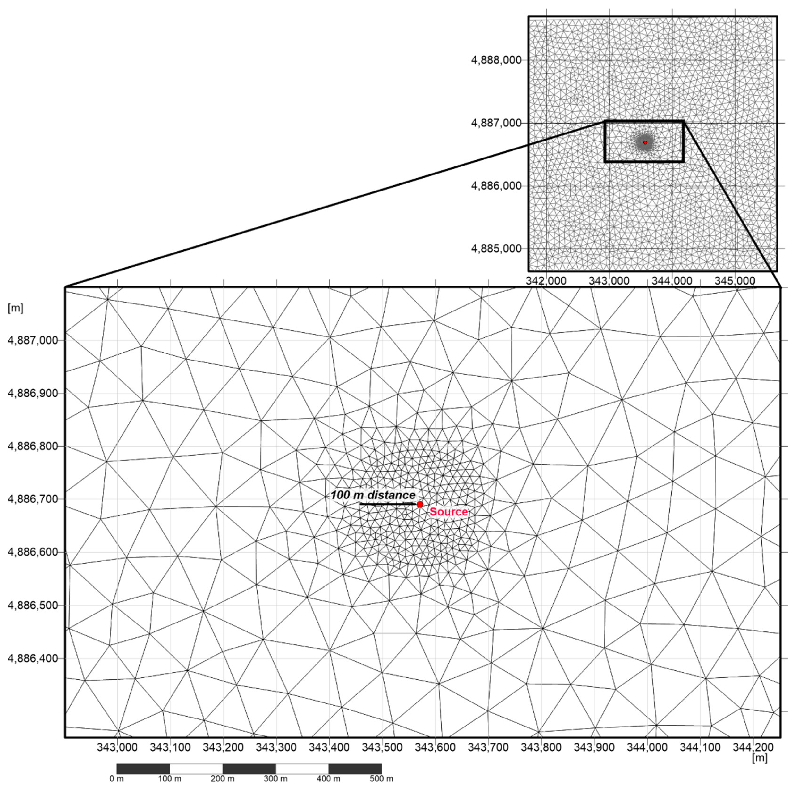
2.1. Study Area

The Adriatic Sea is a semi-enclosed basin in the Central Mediterranean Sea, landlocked on the northern, eastern, and western parts. It is located between Italy and the Balkan Peninsula. The basin is linked with the Eastern Mediterranean Sea in its southern part through the Strait of Otranto, where the main water exchange occurs with an inflow along the eastern coast and an outflow along the western boundary [30].
The distinguishing feature of the north-central Adriatic Sea is a wide shelf reaching a maximum depth of ~100 m in its northernmost section, and an average depth less than 200 in its middle part. The basin position, enclosed by land, highly influences the circulation and the distribution of Adriatic Sea water masses, which strongly depend on the seasonal and inter-annual variability of wind regimes, air-sea and lateral (i.e., river runoff) fluxes. A prevalence of Mediterranean inflow, mainly due to southerly winds, characterizes the winter circulation, while the summer one is driven by a slightly stronger outflow of fresher water (e.g., [31]).
In the present work, we selected two platforms (Plt A and Plt B, hereinafter) located in the north-central Adriatic Sea on a bottom depth of ~45 m, at a ~25 km distance from the Italian coast (Figure 1).

2.2. Model Settings and Input Data

In order to simulate the transport and fate of PW particulate matter discharged from offshore platforms, we here applied the MIKE 3 FLOW MODEL HD FM and the MIKE 3 Particle Tracking (PT) modules, developed by DHI software [32,33], both commonly used for applications in marine coastal environments [34,35,36]. In particular, here we use the MIKE 3 HD to simulate the hydrodynamic circulation in the Sea study area, and then run the MIKE 3 PT, in a decoupled mode based on the pre-calculated hydrodynamic inputs, to simulate the PW suspended matter transport processes.
MIKE 3 HD computes the numerical solution of the 3D incompressible Reynolds Averaged Navier–Stokes equations (RANS), assuming the Boussinesq and hydrostatic pressure approximation, the wind stress based on a drag formulation [37,38], the Smagorisnky formulation for the horizontal eddy viscosity [39,40,41,42] and the κ–ε turbulence model for the vertical [43,44].
The model, based on a flexible mesh approach, allows use of open boundaries (forced by constant or varying elevation, speed, salinity, temperature) under Flather type conditions [45,46], a sigma coordinate system, or a combined sigma and z-layer vertical distribution, and a spatial discretization obtained using a cell-centered finite volume method. The model may also compute heat exchange, evaporation/precipitation, wind stress, wave radiation stresses, etc. [32,33]. Wave–current interactions are not considered in the present work.
In the present model implementation of MIKE 3 HD, we considered the density as a function of temperature and salinity (baroclinic conditions) and a triangular mesh with increasing resolution around the discharge sources: 100 m as maximum mesh side and 15 m as minimum mesh side around the discharge source (Figure 2). The grid covered a square area of about 16 km2 around each platform installations. The boundary and initial conditions (temperature, salinity, currents, and sea surface elevation) derive from the AFS (Adriatic Forecasting System) with a spatial resolution of 1/45° (2.2 km) and 31 σ-levels along vertical direction [47,48]. Initial and boundary conditions were downscaled from the AFS grid to the grid used in MIKE 3 HD. The same grid was used to simulate the PW particulate matter transport process with MIKE 3 PT. Both models applied (MIKE 3 HD and AFS) has been successfully used and validated in the interested area (e.g., [47,48,49]). Given the limited extension of the hereby implemented high-resolution model, the local circulation, temperature, and salinity patterns are strictly related to the patterns simulated by the AFS model. The validation of the AFS model can be therefore clearly extended (from a hydrodynamic perspective) to the local MIKE 3 model, which is capable of properly reproducing the patterns resolved by the parent model in the downscaling procedure. The atmospheric forcing was provided by Climate Forecast System Reanalysis (CFSR), developed, and maintained by the National Centre for Environmental Prediction (NCEP), at an hourly frequency with a spatial resolution of 0.5° for Relative Humidity and Precipitation, and 0.2° for wind, pressure, air temperature and clearness [50].
The 3D hydrodynamic module was run in hindcast mode for the period 1–31 October 2017, corresponding to the monitoring survey time (see Section 3.1), and provided the hydrodynamic input for modeling the transport and fate of PW suspended substances discharged from the two selected platforms.
The MIKE 3 PT module is based on a Lagrangian discrete particle approach; it allows to simulate the particle dispersion and bottom deposition processes, parameterized by means of a random walk using the Langevin equation, as well as the wind forcing, settling, buoyancy, and erosion for non-conservative tracers. The PT module considers the tracer particles as divided into a number of classes, each one characterized by specific properties (decay, settling velocity, density, age, dispersion, erosion) set by the users.
For each particle class, MIKE 3 PT computes the individual particle position at the subgrid scale, thus providing, as output results, the trajectories of the material discharged and the concentration of the suspended discharge components in the water column and on the seabed. The model reproduces the transport of discharged particulate matter from the time of release to initial settling on the sea bottom.
We also assume to neglect decay and flocculation effect, thus treating the particles as conservative tracers and providing a conservative estimate of the potential seafloor depositions. The literature studies [51] showed that some metals present in solution in the PW, after being discharged in the ambient seawater, undergo flocculation processes. The observed transformations of these metals occur on timescales of the order of hours (24 to 160 h) with a sedimentation rate of the new aggregated particles (≈5 mm in diameter), on the order of 0.001 m/s. These timescales appear to be insignificant, compared to the precipitation events close to the interested discharge area, thereby the flocculation process was neglected in the present study.

3. Simulated Scenarios and In Situ Data

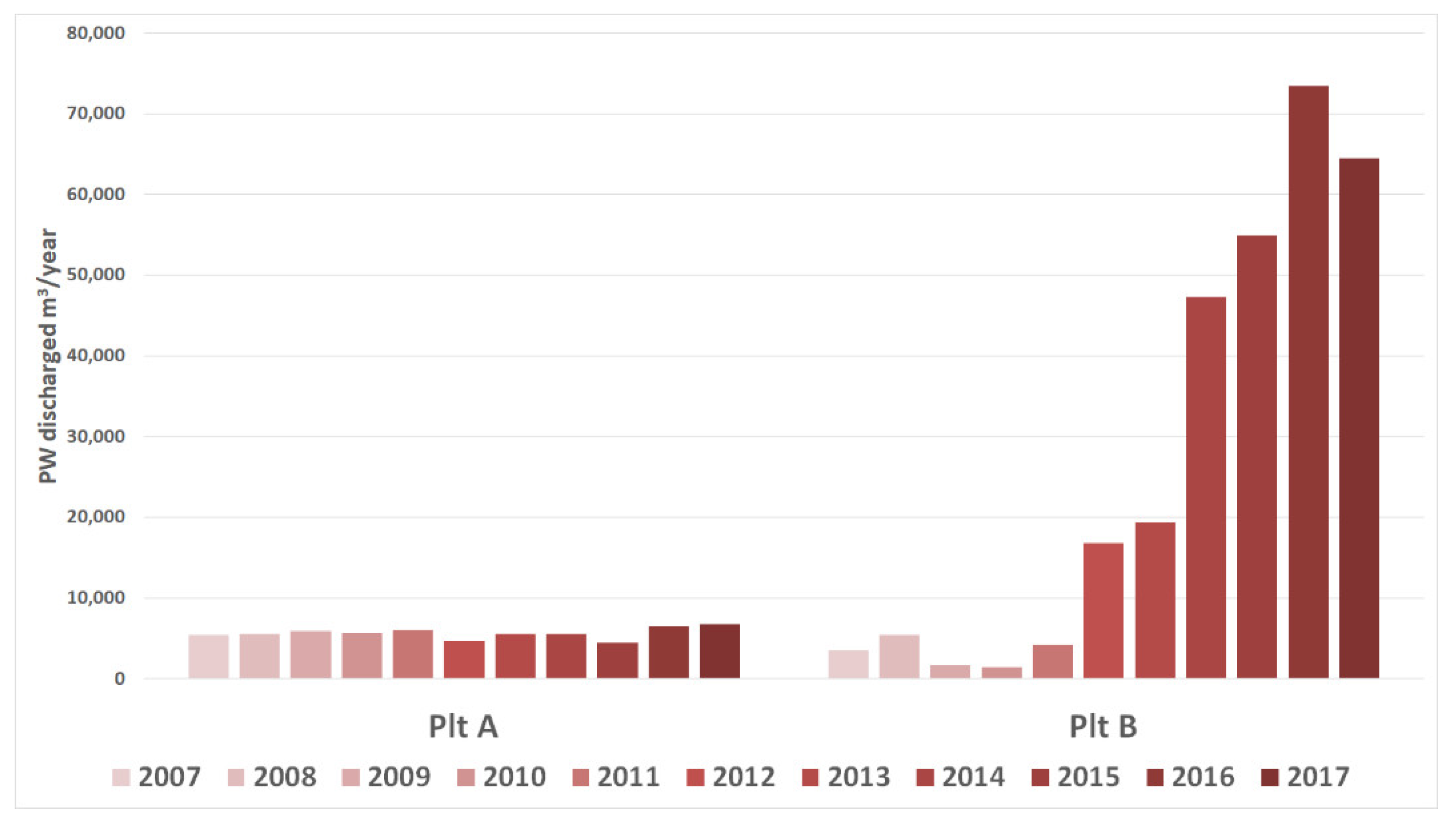
3.1. Discharge Simulation Scenarios
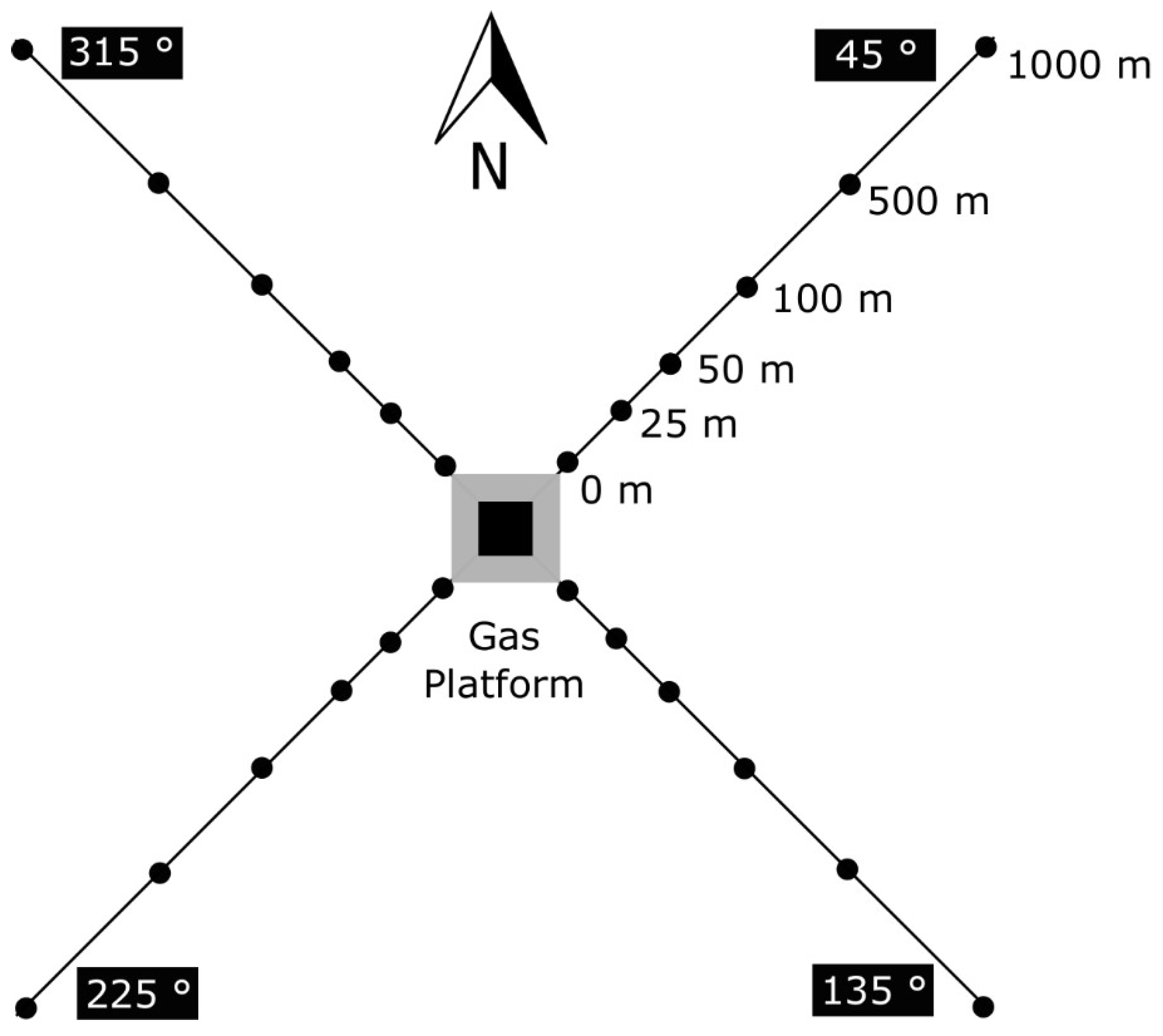
We run the PT simulations for the PW discharged from Plts A and B (Figure 2) as point sources, located in the first 20 m of the water column (see Table 1 for the PW source features).
The particles discharged are considered as divided into three different size classes (sand, silt, and clay) as resulting from the granulometric analysis (see Section 4.1). The three particle classes are set as varying in time discharge sources, to reproduce the real PW volume flux. In fact, on the basis of the PW treatment system, the activation of the discharge occurs with an automatic overflow mechanism, and it is not possible to know its real discharge frequency. Based on this information, a simulated source, discharging continuously for 7 h per day, has been set for both platforms. To properly account for the initial dispersion associated with the random walk approach, the particles dispersion coefficient in horizontal and vertical directions was set as 0.1 m2/s and 0.0 m2/s, respectively (i.e., only the turbulence plays a role in the vertical). For each particle class, the vertical settling velocity (Table 2) has been calculated from the density values available in the literature [16]. The PW flow rate and mass discharge have been calculated from the total PW volume discharged for each platform (Technical Annual Report Schedules B/2, 2017. D.M. AMB. 28 July 1994) considering a continuous 7 h per day discharge and the total amount of TSS resulting from PW analysis (see Section 4.1).
The field measurements have been carried out during the oceanographic survey of October 2017; in situ data were collected along four transect perpendicular to the platform, where six sampling stations per transect were located at increasing distance from the discharge source (Figure 3).
Plt A was characterized by PW volume discharges lower than Plt B (Table 1 and Figure 4), but with clear anomalies in sediment contamination levels registered from 2009 to 2017 around this offshore installation, in particular as regards the level of some organic contaminants detected at the station closer to the discharge source (Table 3). By contrast, Plt B discharged high PW volume in the period 2017 (Table 1 and Figure 4) without highlighting environmental criticality during the monitoring programs conducted so far [5].

3.2. PW Sampling

PW were sampled downstream of the treatment plant, collected in polyethylene bottles for Total Suspended Solids (TSS) analysis (4 L of PW for each platform), and in a dark glass bottle for the particulate matter granulometric analysis (4 L of PW for each platform). Both types of samples were stored at +4 °C until the analysis, carried out as soon as possible, in order to minimize possible chemical, physical, or biological variations during storage.

3.3. Total Suspended Solids (TSS)

Whatman GF/F filters with a porosity of 0.70 μm and a diameter of 45 mm were used to estimate the TSS content of PW. Before use, the GF-F filters were placed in an oven at 105 °C for one hour, left to cool in a dryer for 30 min, and then weighted with a 5-digit decimal balance, numbered, and stored in the filter holder. After a previous homogenization, 2 L of PW were filtered under vacuum on GF-F pre-treated filter. Before its removal from the filtration ramp, the filter was washed three times with distilled water (10 mL at a time) and held under vacuum for another three minutes. Once filtration was complete, the filter was transferred to an oven at a temperature of 105 °C for one hour, left to cool in a dryer for 30 min and then weighed to determine the amount of the retained solid (TSS) in the samples water.

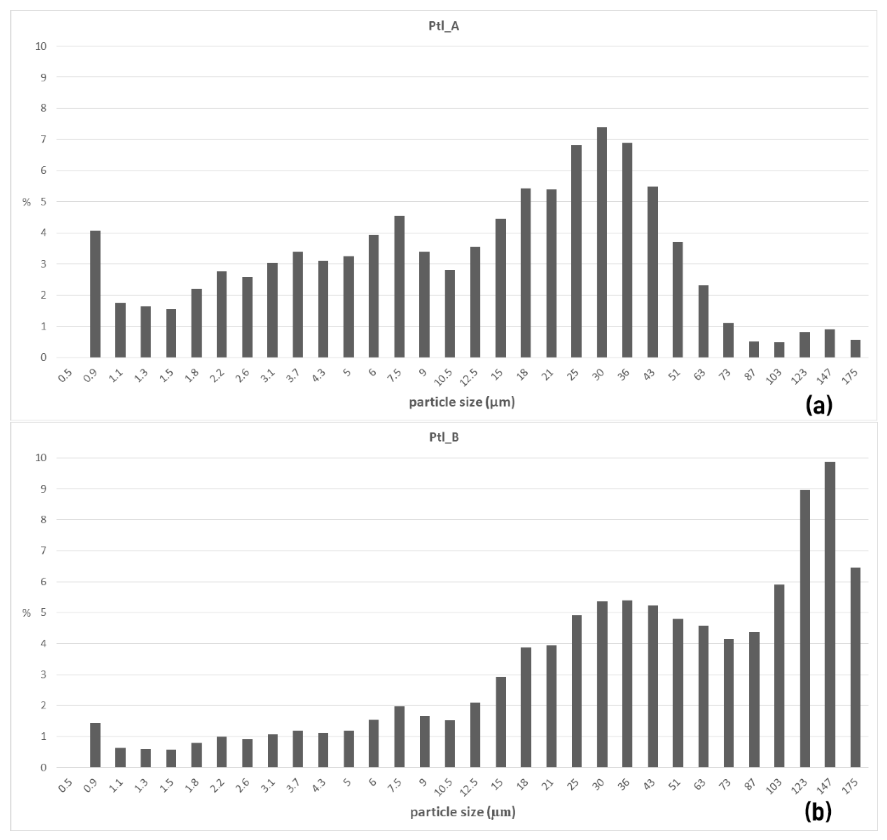
3.4. Granulometric Analysis

The analytical determination of the content and dimensions of the particles contained in the water samples was carried out according to the laser light diffraction method ISO 13,320 [54,55]. The method involves a pre-treatment phase of the sample with hydrogen peroxide and subsequent granulometric analysis by laser diffraction.
In order to eliminate salts and organic substances that may cause problems during the analysis, 10 mL of 30% hydrogen peroxide solution was added to 200 mL of PW sub-sample and left to react for 48 h under a hood. An aliquot of the pre-treated sample was placed in an oven at 50 °C in a previously weighed capsule, left for the time necessary for the complete evaporation of the water from the residue, and then it transferred to the dryer until constant weight.
The sample residue was recovered with about 15 mL (±0.5 mL) of sodium hexametaphosphate solution (1 g sodium hexametaphosphate dissolved in 2 L of distilled water), stirred, and then left to stand for at least 24 h at room temperature. In the end, the sample was subjected to an ultrasonic water bath for 60 s to eliminate any air bubbles, and then transferred to the instrument cell for granulometric analysis.
The instrumentation used was a Sympatec HELOS laser diffraction particle analyzer, with the possibility of installing up to five interchangeable measuring lenses (Fourier lenses), in order to divide the measuring range into different intervals allowing particles size from 0.18 µm to 875 µm to be measured. After a reference reading performed with distilled water, the sample was introduced into the instrument cell in small quantities until the optical concentration inside reached values between 15–30% suitable for the correct reading of the sample.

4. Results and Discussion

4.1. PW Analysis

The results of the TSS analysis showed that the suspended solid material content in the PW of Plt A was three times higher than that of Plt B (Table 4). The results obtained from the particle size distribution analysis (Figure 5) showed that both samples were characterized by a higher abundance of the fine fraction than the coarser one. In particular, the fine fraction (silt plus clay) represents about 96% of the TSS contained in the PW of Plt A and about 60% of TSS contained in the PW of Plt B.

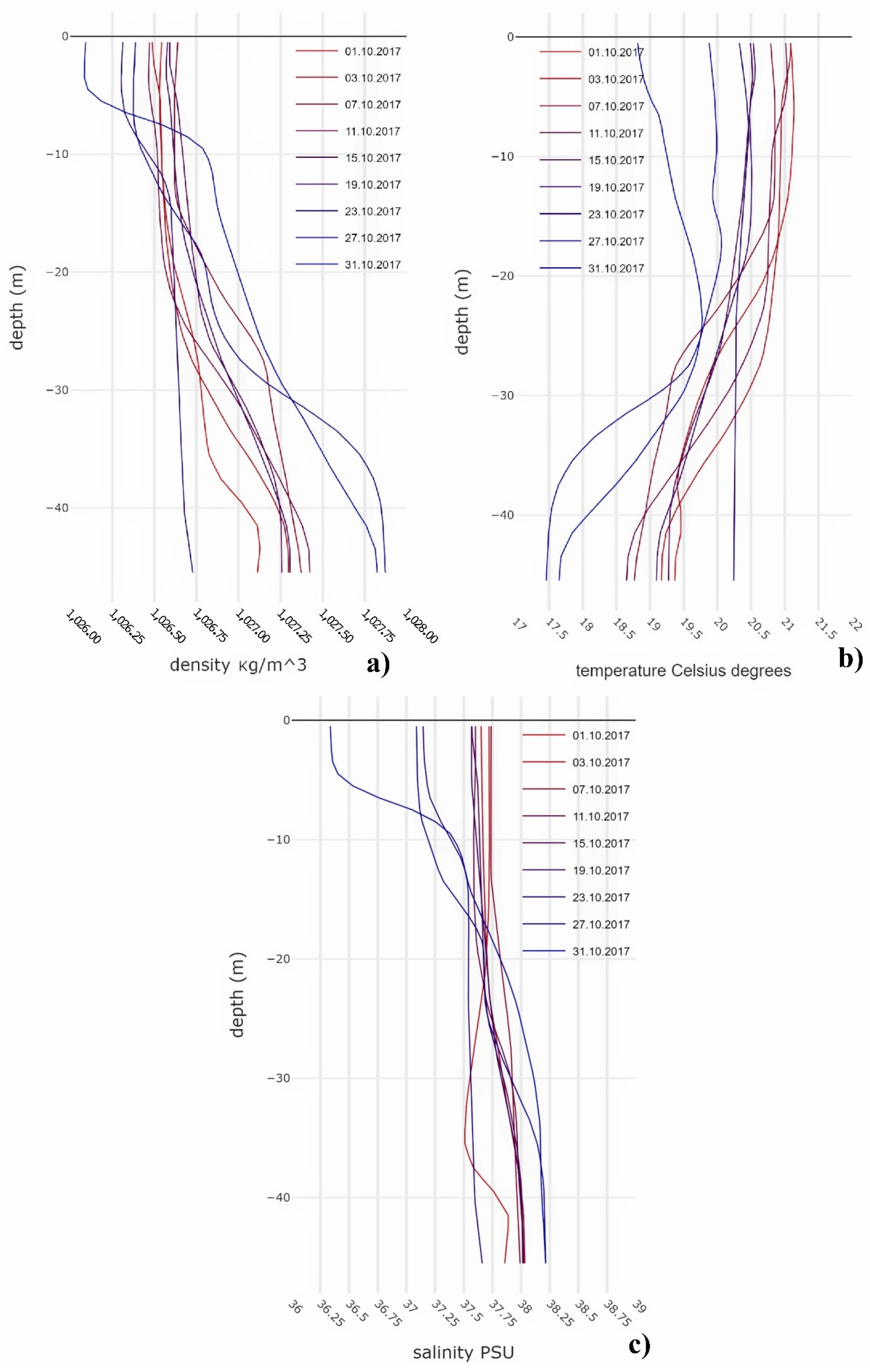
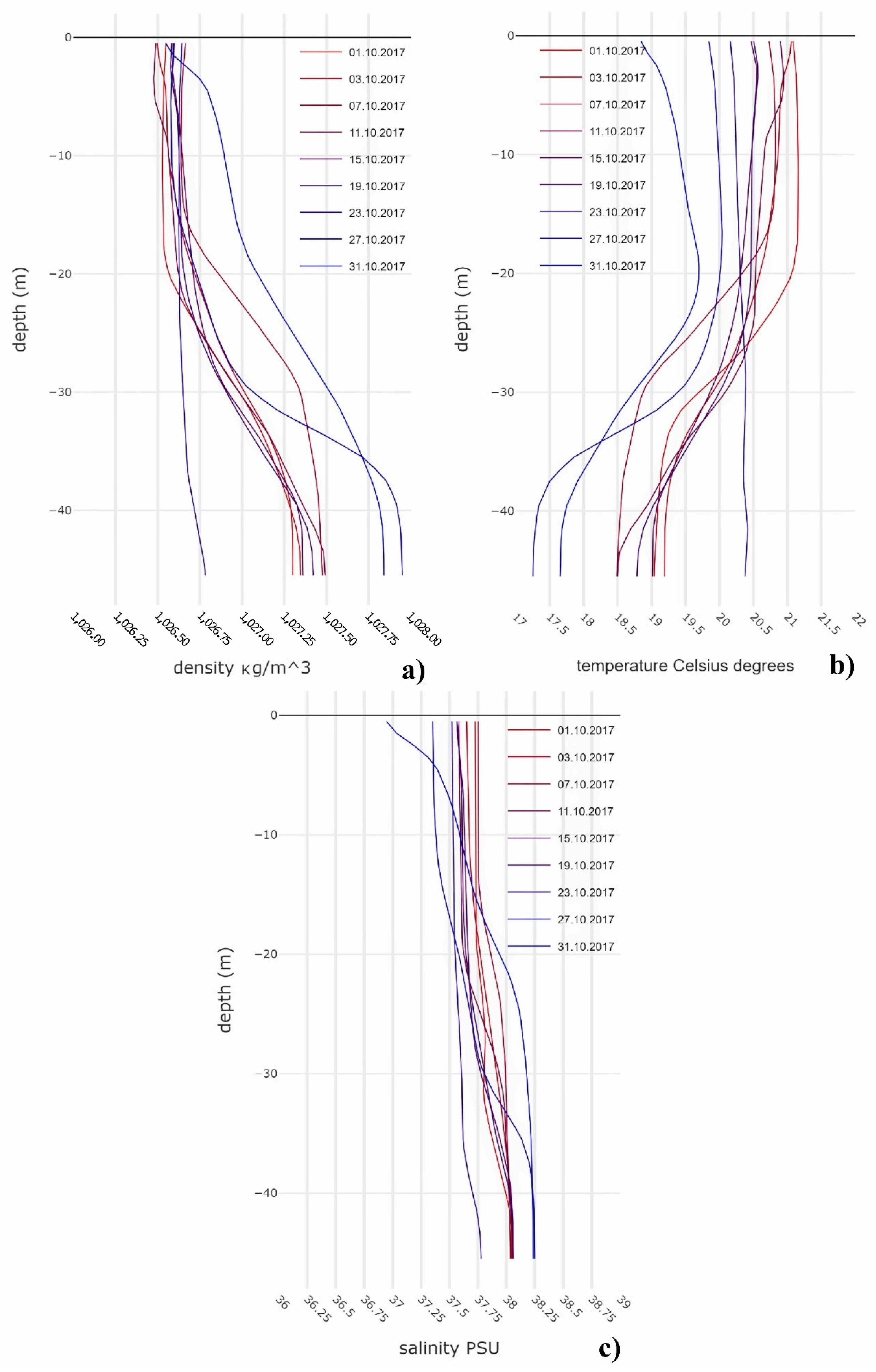
4.2. Hydrodynamic Conditions

The salinity, temperature, and density profiles from MIKE 3 HD (Figure 6 and Figure 7) showed the features of the water column, around both Plt A and B, during the simulation period 1–31 October 2017. In the neighboring of Plt A, over the first 20 days of October, the water column was characterized by a weak stratification condition, with the salinity and temperature values in the range 37.75–38.25 and 18.5–21.2 °C, respectively (Figure 6a,b). In the last 10 days of October, a density stratification condition became clear, with a fresh water mass intrusion in a subsurface layer (between 0 and ~5 m) (Figure 6a,c).
The hydrological parameters profiles (Figure 7a–c) around Plt B showed an almost homogeneous distribution in the water column, with an initial stratification condition occurring only at the end of October as observed for the Plt A area (Figure 7a).
The analysis of current fields computed by MIKE 3 HD during the simulation period at three different depths (surface, discharge, and bottom depth) at Plt A and B are presented in Figure 8. In the monthly simulation period, the most intense currents at both Plt A and B were observed primarily in the surface layer and at discharge depth (10 m), with maximum speeds in the range of 0.4–0.7 m s−1 (Figure 8). The prevalent direction at the three different depths was towards the SE sectors, while currents towards the SW and NW directions were much less frequent and less intense (≤0.2 m s−1) At both platforms sites, currents at bottom depth were much less intense (<0.2 m s−1) for all the sectors.

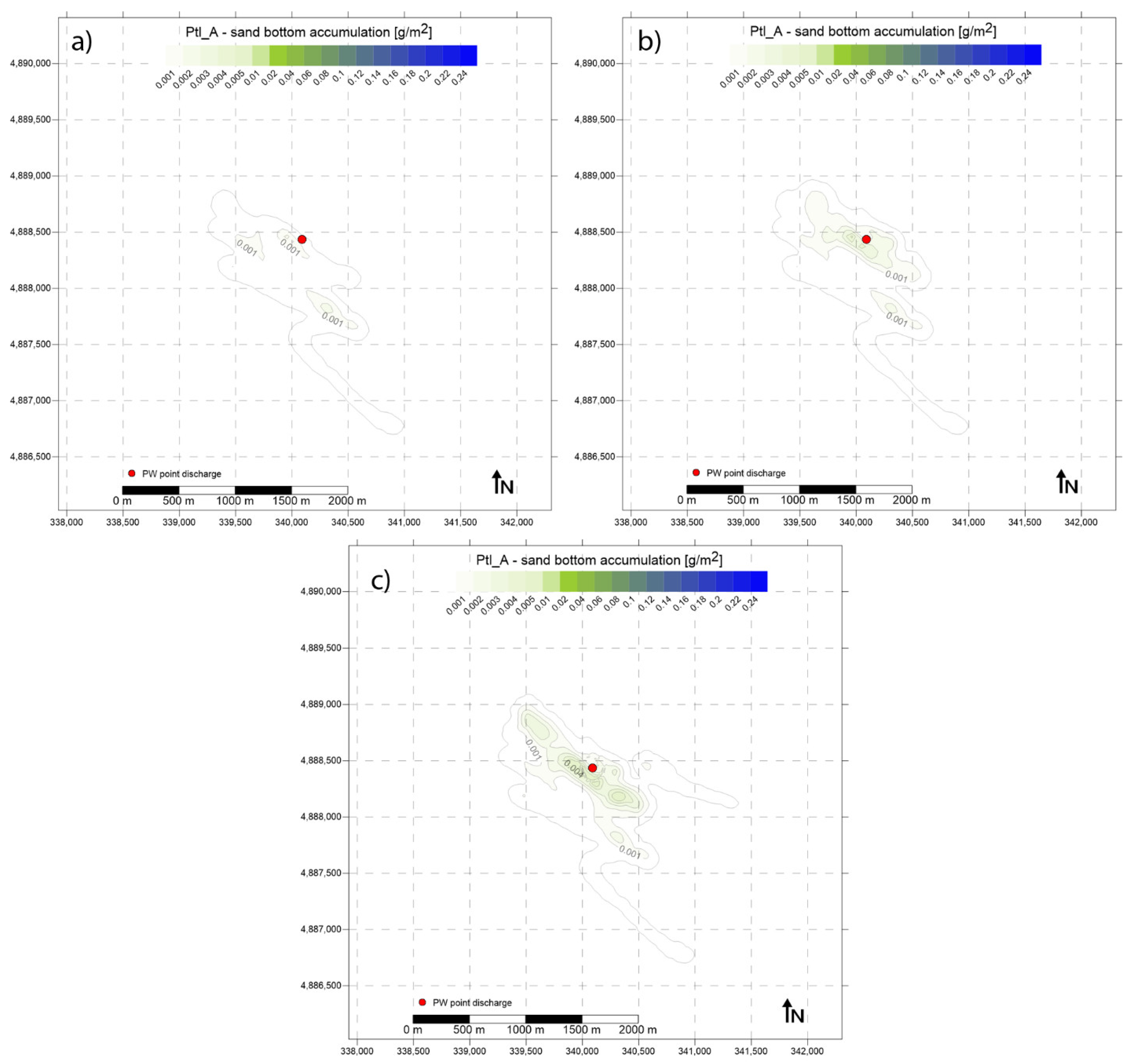
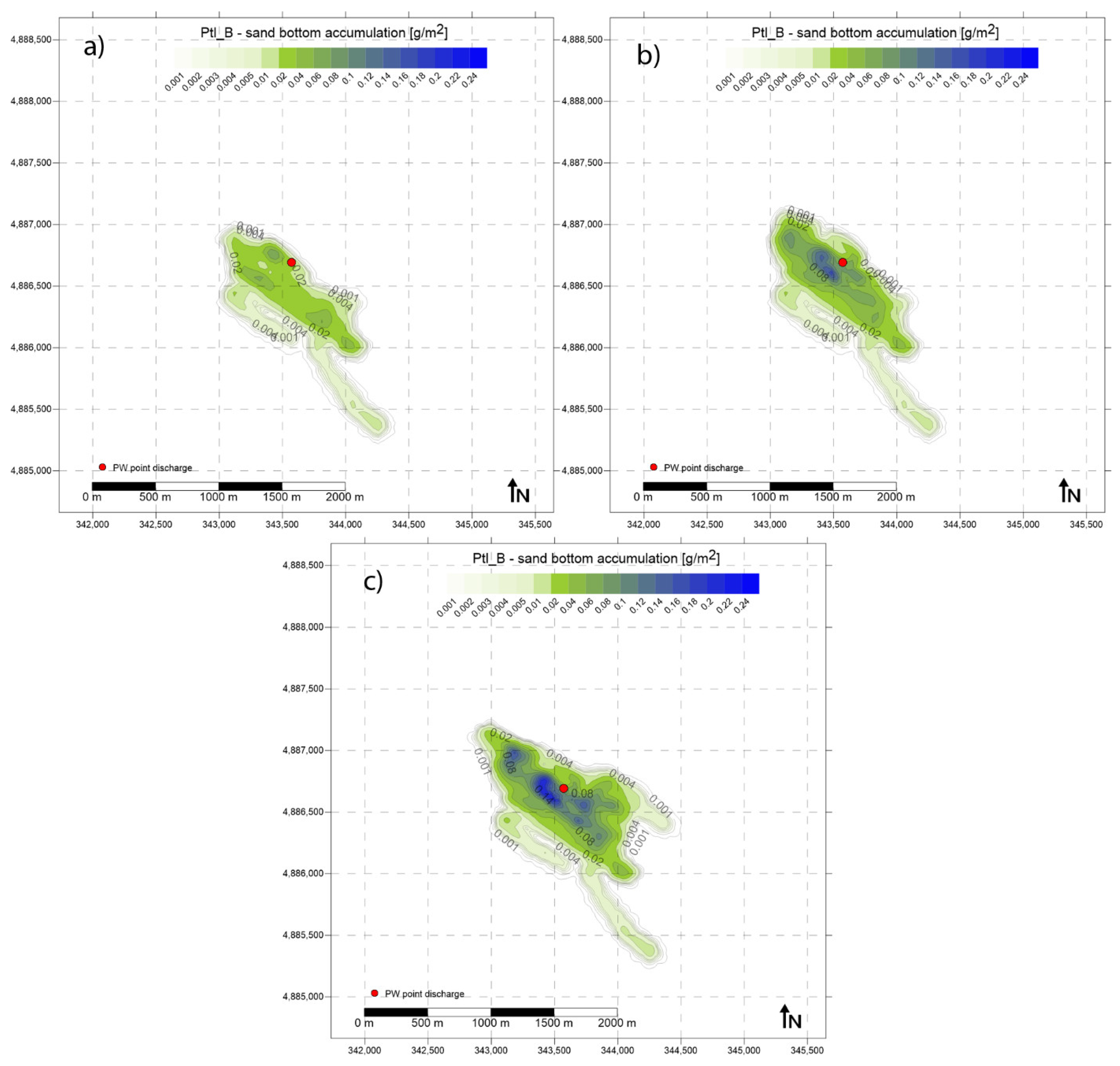
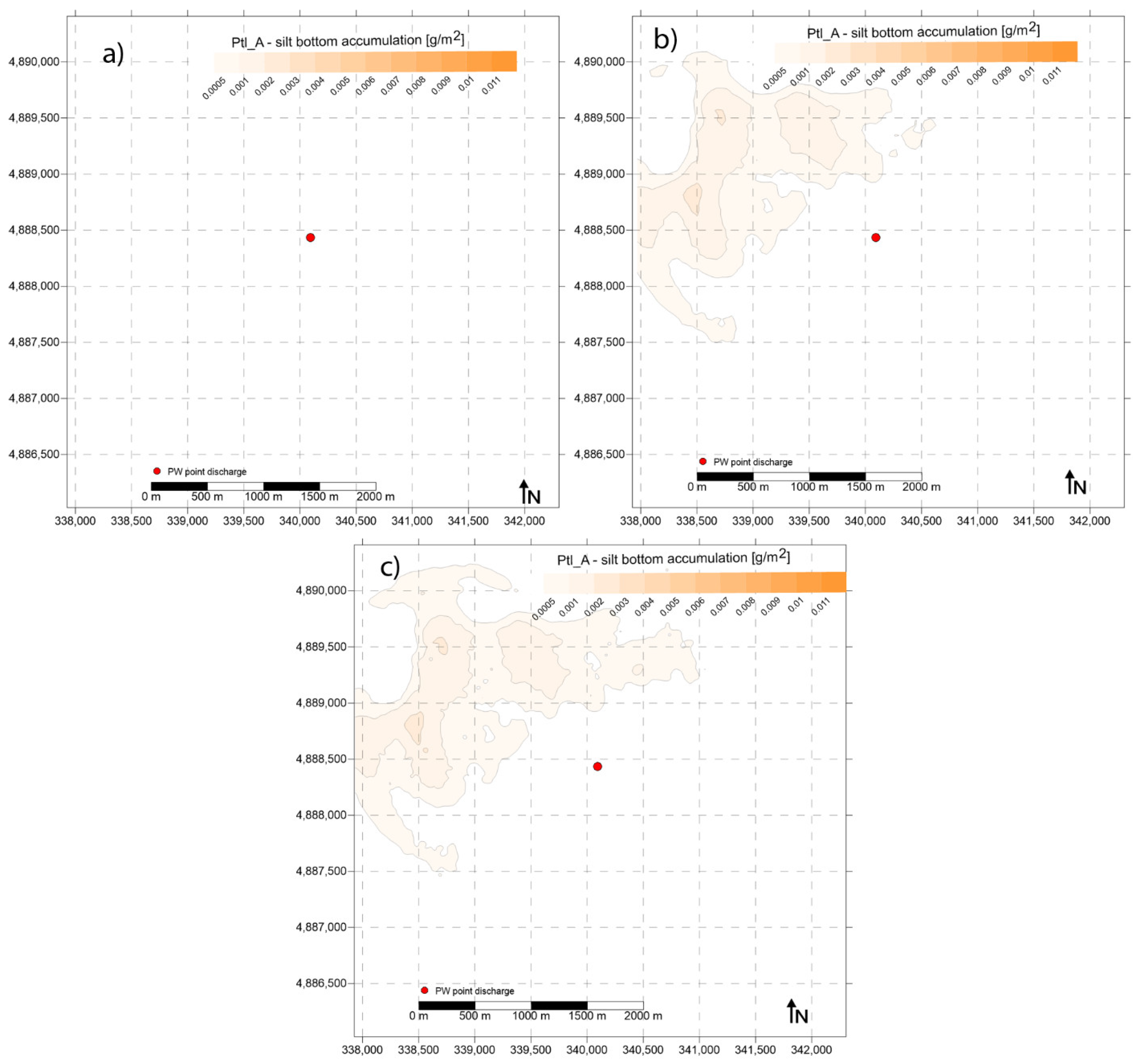
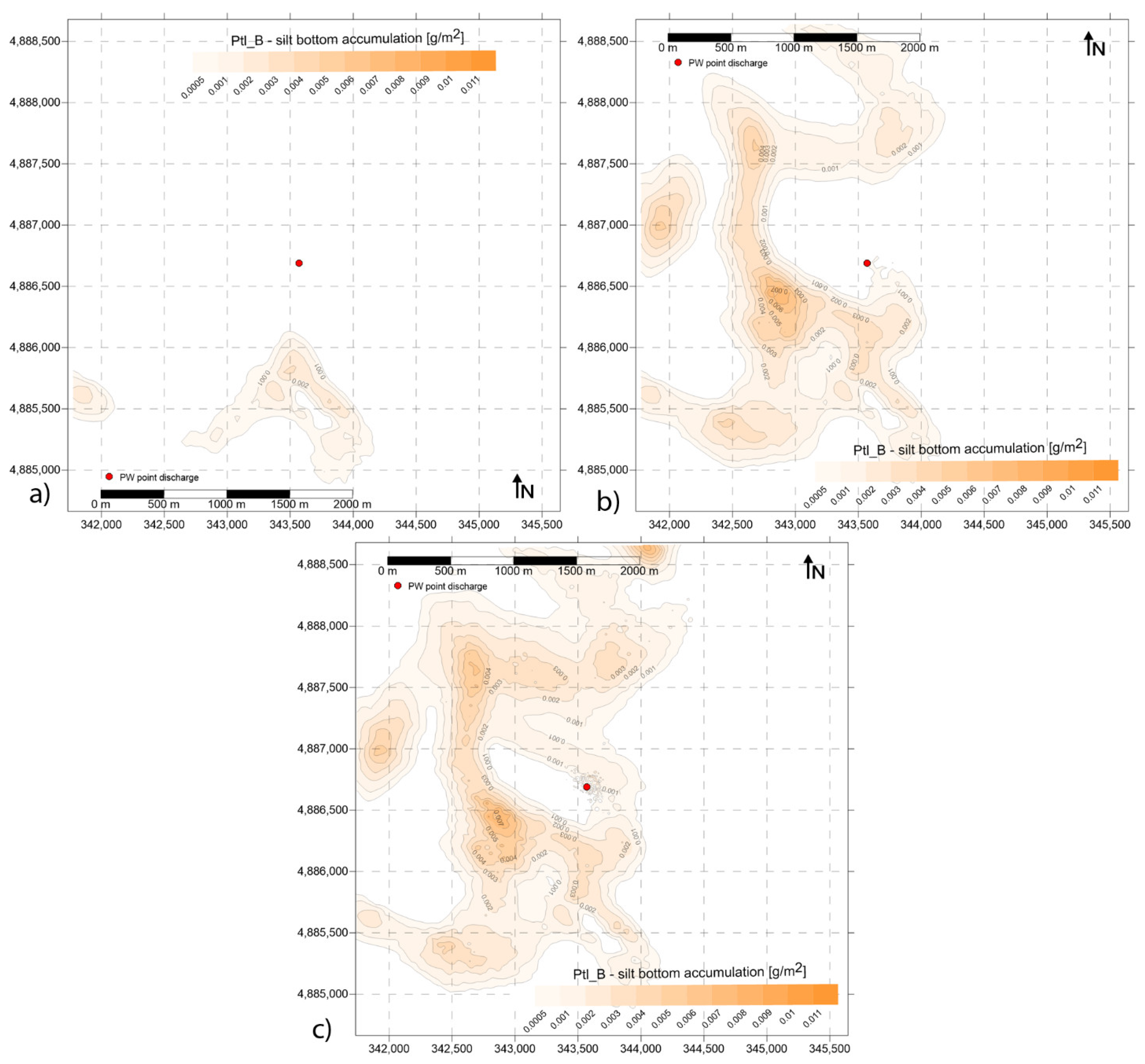
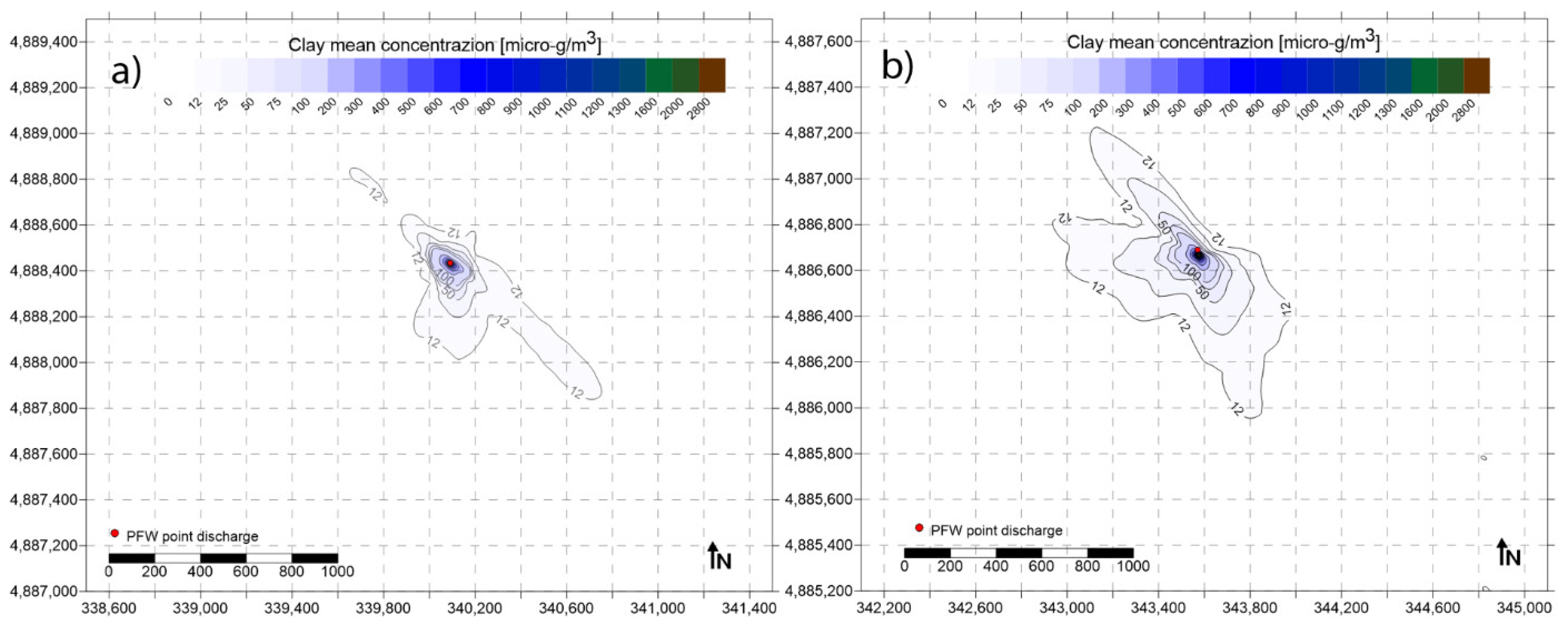
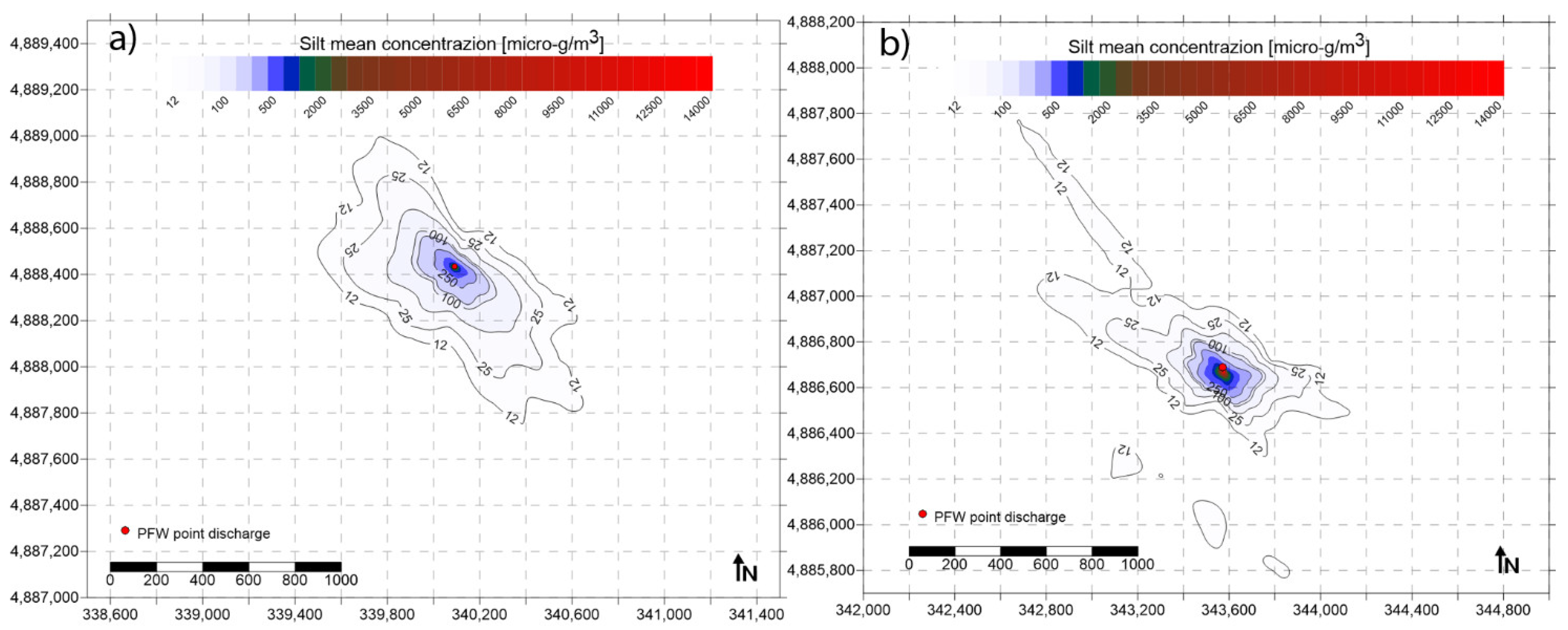
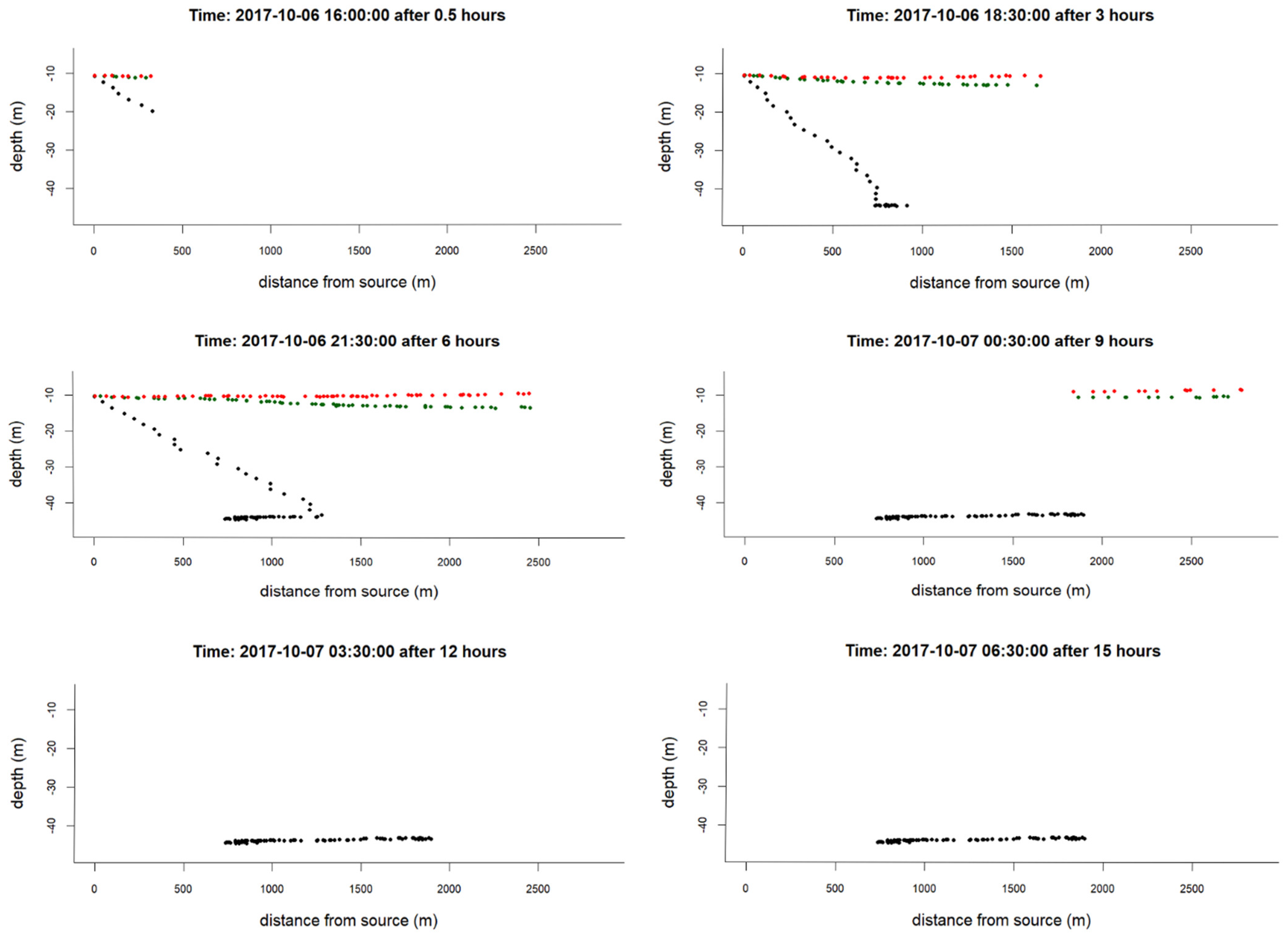
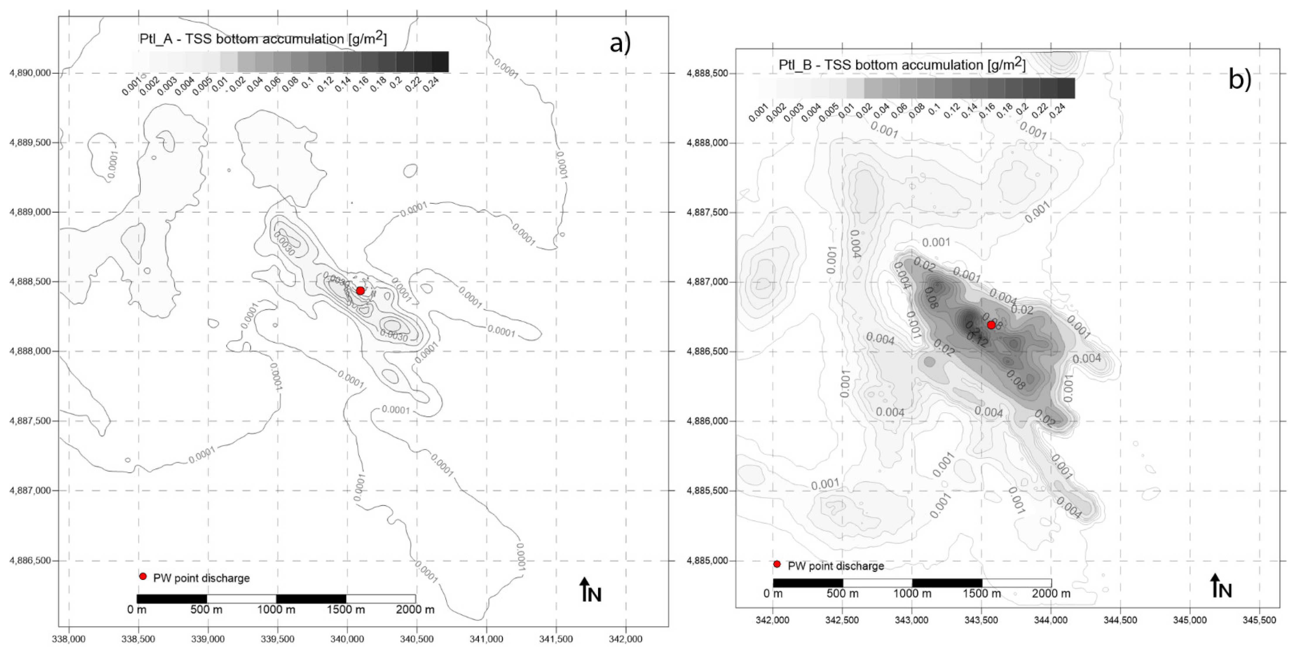
4.3. Transport and Fate of PW Particulate Matter Discharged

During the monthly simulation, based on the hypothesis of a continuous discharge of 7 h per day, Plt A released at sea about 585.9 m3 of PW containing a total of 37.35 kg of TSS, while the Plt B, during the same time interval, discharged about 5520.5 m3 of PW containing a total of 113.77 kg of TSS. Table 5 provides the total amount of TSS discharged from both platforms, split into the three particulate size classes. The amount of TSS discharged from Plt B is about three times the amount discharged from Plt A. In accordance with the characterization and the granulometric distribution of TSS in the PW (Table 4 and Figure 5), silt represents the predominant discharged component for both structures.
The simulations of the transport processes of TSS discharged along with the PW, showed a clear separation between the behavior of coarser particles (>63 microns) compared to the smaller ones (<63 microns). Table 6 reports the quantities of TSS that reach the seabed, within an area of 16 km2 around the source, and those that remain in suspension for each granulometric classes considered. In the Plt A case, only 16.5% of TSS discharged settled on the seabed, while in the Plt B case, due to the greater abundance of sand in the PW, almost 50% of TSS discharged with PW reached the bottom. At both platform sites, the behavior of the different grain size classes showed that 100% of the sand reached the seabed, less than 20% of silt settled on the bottom and 100% of clay remained in suspension in the water column and did not accumulate on the seabed around the studied area during the 31 days of the simulation run. Figure 9, Figure 10, Figure 11 and Figure 12 show, for the three particle size classes, the bottom accumulation around both platform areas, after 10 and 20 simulation days and at the end of one month as resulting by MIKE 3 PT output.
The sand particles, after the discharge, spread within a horizontal distance of about 1500 m from the source along the NW-SE direction (Figure 9 and Figure 10) for both platforms, according to the currents intensity and directions in the deepest layer, as computed by the hydrodynamic model (Figure 8). The maximum concentration of sand settled on the seabed around the Plt A (Figure 9) after one month of discharge activities, amounted to 0.0078 g/m2 and was transported by the flow fields within a distance of about 150 m from the discharge source, along the NW-SE direction. Higher sand accumulation values were found around the Plt B (Figure 10) with a maximum concentration of 0.2346 g/m2 spreading within a distance of about 170 m from discharge point, along the NW-SE direction as in the case of Plt A.
The silt (Figure 11 and Figure 12) and clay (not shown) discharged with PW, tended instead to remain suspended in the water column and to be transported by the currents outside the model domain. The small percentage of silt reaching the bottom was advected in the NW sectors of the study area around platform A (Figure 11), while around platform B a more variable distribution, covering the NW and SW sectors, may be observed (Figure 12). The silt bottom accumulated around both platform areas presented very low concentration values with the maximum values of silt settled concentration of 0.0023 g/m2 and 0.0082 g/m2 for Plt A and for Plt B, respectively.
Figure 13 shows the mean concentration of suspended clay around the platform areas calculated on the monthly simulation results at the discharge depth (Table 1), where the maximum concentration has been observed. The clay did not reach the seabed, but it remained in the suspension being advected by the current field and spreading within about a 700 m radius around both platform structures. The mean concentrations of the suspended clay around both discharge areas showed very low values in the range of 12–40 µg/m3. Slightly higher average values were displayed for Plt B discharging a PW volume about ten times that of Plt A. In the proximity of the source point, within about 3 m for Plt A and 23 m from Plt B, the mean concentrations reached values equal to 2.6 µg/L for Plt A and 3.3 µg/L for Plt B, while the maximum concentration computed during a whole month of the simulation was equal to 30 µg/L for Plt A and 38 µg/L for Plt B (Table 7).
Similar behavior may be observed for the silt, both in terms of the affected area extent and the mean concentrations of suspended particulate materials detected around the source (Figure 14). The highest mean silt concentration may be observed within a few meters from the source (about 3 m for Plt A and about 23 m for Plt B), at the same distance at which the highest clay suspended concentration values were detected too, but with slightly higher concentration values corresponding to 6.8 µg/L for Plt A and 18 µg/L for Plt B, respectively. The maximum silt concentration observed during the month of the simulation was 77 µg/L for Plt A and 191 µg/L for Plt B (Table 7).
The time series of suspended clay and silt concentration (Figure 15a for Plt A and Figure 15b for Plt B), at the point where the max concentration of TSS fine fraction was computed during the discharge simulation, showed that the higher concentration in the water column, close to the source point, corresponding to a very low current intensity condition. The variation in TSS suspended distribution therefore mainly depended on the intermittent discharge, as shown in Figure 16, and on the intensity of the current field at the discharge depth.
The vertical cross-section of the PW fate (Figure 16 and Figure 17) shows the trajectories and deposition on the seabed of the particulate matter associated with the PW plume during a single discharge event. In the case of Plt A (Figure 16) the discharge depth was 10 m and the hydrodynamic conditions determined the rapid dynamic of this release scenario (Table 8). In less than one hour after the release began, the particulate matter discharge separated into two groups of particles: the first one appeared to spread horizontally and consisted of silt and clay particles, with very small diameters and negligible sinking velocities. This finer portion of the TSS discharged with the PW remained in suspension at approximately the same depth at which it was released and, after about 9 h from the discharge activation time, spread out of the model domain. The other group of particles began sinking down towards the seabed and consisted of sand particles, coarser than the first group and with relatively large diameters. In a little more than two hours, after the end of the discharge activity, the initial discharge conditions were restored. For Plt A, the distance from the source, at which the sand reaches the bottom, varied from a minimum of 700 m up to almost 2 km.
Furthermore, in the case of Plt B (Figure 17), after half an hour from the start of the discharge activation, the TSS associated with the PW had already undergone a separation between the sand, which tended to sink down, and the lighter materials (silt and clay), that remained in suspension and were horizontally transported due to the advection and dispersion processes. In a little more than two hours, the sand particles reached the sea floor and started to settle at a distance of about 500 m from the source. During this discharge event, silt and clay showed a similar behavior and both tended to move away from the source at about the same depth of the discharge point. After eight hours from the end of the discharge activity, all the sand had already settled, while the finer part again spread in the water column. After about 15 h from the initial discharge, also the finer TSS parts left the neighboring of Plt B and the environmental situation around the source returned to the initial condition. Around both platforms, independently from the discharge source depth (10 m Plt A, 20 m Plt B), the time required for the sand to reach the sea floor was about 2 h.
The distribution map of the amount of TSS (silt plus sand) accumulated on the seabed around the Plt A (Figure 18a) after one month of discharge activity shows very low accumulation values even around the source, influenced almost exclusively by the sandy component and with a maximum accumulation value of 0.008 g/m2 within a distance of about 150–300 m from the source. In the case of Plt B (Figure 18b), the accumulated mass on the seabed was slightly higher with a maximum mass accumulated of 0.2346 g/m2 in one month of discharge activity at about 170 m distance from the source.
The one-month long simulation performed with MIKE 3 HD reproduce current fields with intensities values in a range from a minimum of 0.2 m/s to a maximum of 0.7 m/s and prevalent directions toward the SE sector in agreement with the main circulation pattern of the northern- central Adriatic Sea where the overall main current is represented by the Western Adriatic Current (e.g., [30,56]).
The volume of PW discharged by the offshore platforms varies greatly from one platform to another [57,58], while the TSS contained in the PW may change based on the type of reservoir and upstream PW treatments (minimum 4 mg/L; maximum 746 mg/L, median 94 mg/L; Technical Report Schedules B/2, 2010–2017 D.M. AMB. 28 July 1994). The two selected platforms are characterized by different features of PW discharge (Table 1) but present slightly different contents and particle size distribution of the TSS. Throughout the one-month simulation period, the different features of the two platforms’ discharge do not seem to drive the mid-term dispersion of TSS, which is mainly influenced by the hydrodynamic conditions and intermittent discharge activity according to modeling studies previously conducted in the same area [24].
The TSS (silt and clay) dispersed from both the platforms in the water column, never showed particularly high concentration values compared to the amount of suspended particulate matter naturally present in the Adriatic Sea [59,60]. Literature studies suggest, for the northern Adriatic Sea, the concentration of 3 mg/L TSS as a threshold value to discriminate water masses influenced by fluvial inputs from offshore waters, which are generally characterized by values between 0.5 and 3 mg/L TSS [61]. In the same Adriatic area, other studies indicate average TSS concentrations, measured in high salinity water masses not influenced by river input, between a minimum of 0.47 ± 0.72 mg/L and 1.81 ± 1.56 mg/L during different seasons [62]. It is also worth noting that the finest particles (diameter < 63 micron) represent the size fraction which is typically most involved in adsorption phenomena of organic and inorganic substances due to the relatively higher surface area and the compositional characteristics of the fine particles [63,64,65,66]. Compared to the literature TSS concentration values, the average silt and clay concentration resulting from the PW discharge simulation is less than one or two orders of magnitude. The maximum values of silt and clay concentration are also lower than the minimum values of particulate matter found in the northern Adriatic Sea [62].
The data of mass accumulated rates (MARs) available in the literature for the Adriatic Sea show a wide range of values from 0.03 to 6.6 g cm−2 yr−1 [67,68,69]; the highest values were reported only for the delta areas of the main rivers (Po and Isonzo), while the most abundant class of MARs is represented by values between 0.04 and 0.06 g cm−2 yr−1 [67]. More specifically, in the area around the investigated platforms, the average accumulation rate reported is about 0.15 g cm−2 yr−1 [67].
With the aim of comparing the MARs literature data and the values resulting from the simulation of the monthly discharge activity, we scaled the numerical results to the annual values, assuming a 12-month constant discharge activity and adding a precautionary correction factor of 25% to the simulated values. Since the month of October could not be assumed as representative of an entire year hydrodynamic conditions, the correction factor was added in order to perform a more precautionary comparison with MARs literature data. The maximum annual mass accumulation rates computed for the two platforms were approximately 1 µg cm−2 yr−1 for Plt A and 30 µg cm−2 yr−1 for Plt B.
The amount of particulate matter discharged with PW and deposited on the sea floor, within 2 km around the selected platforms installations, consists almost exclusively of the sandy component associated with the PW discharge, which settled affecting the underlying sediment. Compared to the sedimentation rates here reported, a very low amount of particulate matter discharged with PW reaches the seabed close to the platforms and appeared to be several orders of magnitude below the values of sedimentation rates in the literature, therefore, its contribution to the total balance of material settled annually on the seafloor of the investigated areas appears to be negligible. Moreover, the high sediment contamination levels detected, in particular for Plt A, within 50 m from the platform installation, seems to be not consistent with the model results, showing very low sedimentation rates close to the structures and distributed within a radius of more than 1000 m around the PW sources. This would also be confirmed by the lack of correlation between the sediments contamination levels detected around the two platforms, during the October 2017 oceanographic survey, and the mass accumulation rates computed at sediment sampling station sites (Figure 19). Correlation analysis was performed using the Spearman test [70], which is a rank-based correlation coefficient (non-parametric), since the data did not have a normal distribution.
Consequently, the TSS associated with the PW discharges does not appear to be clearly related to the sediment contamination levels observed during the monitoring activities in the neighboring of the platforms selected (Table 2).

5. Conclusions

To the best of our knowledge, this is the first study addressing the transport and fate of the particulate matter discharged in the marine environment with the PW plume generated during offshore hydrocarbon extraction activity. The work was conceived to assess the potential contribution of the total suspended solid, associated with the PW effluent, to the sediment contamination observed in the Adriatic Sea during offshore platforms monitoring programs carried out so far.
To this aim, we apply the hydrodynamic model MIKE 3 HD and the Lagrangian particle model (MIKE 3 PT), using TSS in situ data collected during October 2017, to simulate one month PW discharge activity from two selected platforms located in the Adriatic Sea. The outcomes show that the fate of the TSS seems to be very similar for both platforms and is mainly affected by the particles size distribution and the environmental hydrodynamic conditions. In the investigated area close to the platform installations, the sediment is affected by the settling of the sand associated with the PW discharge and the TSS showed a negligible contribution to the total balance of material deposited annually on the seafloor. The present results also suggest that at the time and space scales investigated, even in the area close to the discharge point, the amount of TSS released with the PW determines a negligible increase in suspended particulate matter along the water column. The anomalies observed in the sediment contamination levels around the selected platforms thus may be poorly related to the TSS content associated with the PW discharge.
The numerical procedure adopted here, integrating observational data from monitoring surveys, represents an important first step to understand what and how much TSS released with the PW discharge settles on the seabed. It provides an efficient alternative to conducting difficult and expensive field observations and paves the way to extend this study to many different discharge scenarios. This approach also opens to a number of broader perspectives, in terms of risk assessment and mitigation effect arising from TSS discharged with the PW in the marine environment and may play a crucial role in the design of future monitoring programs.

Author Contributions

Conceptualization, R.D.M. and A.P.; methodology, R.D.M., D.C. and A.P.; software, R.D.M.; validation, A.P.; formal analysis, R.D.M., D.C., G.G., P.L., B.D.L. and F.V.; investigation, R.D.M., D.C., G.G., P.L. and F.V.; resources, R.D.M.; data curation, R.D.M., D.C., G.G., P.L., B.D.L. and F.V.; writing—original draft preparation, R.D.M. and D.C.; visualization, R.D.M. and D.C.; supervision, D.C.; project administration, R.D.M. All authors have read and agreed to the published version of the manuscript.

Funding

Daniela Cianelli was partly supported by the Stazione Zoologica Anton Dohrn internal individual research funds. This research has been supported by ISPRA internal research funds.

Institutional Review Board Statement

Not applicable.

Informed Consent Statement

Not applicable.

Data Availability Statement

The data presented in this study are available on request at following link www.isprambiente.it. Accessed date September 2020.

Acknowledgments

Rossella Di Mento and Daniela Cianelli thank Marina. Amici for her support in Production Water chemical analysis and Marco. Uttieri for useful discussion.

Conflicts of Interest

The authors declare no conflict of interest.

References

  1. EIA. Gulf of Mexico Fact Sheet. U.S. Energy Information Administration. 2020. Available online: http://www.eia.gov/special/gulf_of_mexico/ (accessed on 1 September 2020).
  2. WOR. Oil and Gas from the sea. In World Ocean Review: Marine Resources—Opportunities and Risks; Maribus: Hamburg, Germany, 2014; pp. 8–51. Available online: http://worldoceanreview.com/en/wor-3-overview/oil-and-gas/ (accessed on 1 September 2020).
  3. Neff, J.M.; Lee, K.; DeBlois, E.M. Produced Water: Overview of Composition, Fates, and Effects. In Produced Water; Springer: New York, NY, USA, 2011; pp. 3–54. [Google Scholar] [CrossRef]
  4. OSPAR Commission. Discharges, Spills and Emissions from Offshore Oil and Gas Installations in 2017. In Offshore Oil & Gas Industry Series; Publication Number: 740/2019; OSPAR Commission: Sintra, Portugal, 2019; p. 66. [Google Scholar]
  5. Di Mento, R.; Amici, M.; Berducci; Calcagni, L.; Lanera, P.; Maggi, C.; Mannozzi, M.; Lauria, A.; Oteri, F. Technical Reports on the Italian Monitoring Program to Assess the Impact on the Marine Environment from the PW Discharges in the Sea from Offshore Platforms; ISPRA: Rome, Italy, 2009–2017. [Google Scholar]
  6. Tornambè, A.; Manfra, L.; Di Mento, R.; Moltedo, G.; Catalano, B.; Martuccio, G.; Sebbio, C.; Chiaretti, G.; Faraponova, O.; Amici, M.; et al. Application of a ‘weight-of-evidence’ model for assessing sediment quality and associated hazard with offshore gas platforms discharging produced water. In Proceedings of the SETAC Europe 28th Annual Meeting, Rome, Italy, 13–17 May 2018. [Google Scholar]
  7. Manfra, L.; Maggi, C.; d’Errico, G.; Rotini, A.; Catalano, B.; Maltese, S.; Moltedo, G.; Romanelli, G.; Sesta, G.; Granato, G.; et al. A Weight of Evidence (WOE) Approach to Assess Environmental Hazard of Marine Sediments from Adriatic Offshore Platform Area. Water 2021, 13, 1691. [Google Scholar] [CrossRef]
  8. Bakke, T.; Klungsøyr, J.; Sanni, S. Environmental impacts of produced water and drilling waste discharges from the Norwegian offshore petroleum industry. Mar. Environ. Res. 2013, 92, 154–169. [Google Scholar] [CrossRef] [PubMed] [Green Version]
  9. Beyer, J.; Anders, G.; Dag, H.; Jarle, K. Environmental effects of offshore produced water discharges: A review focused on the Norwegian continental shelf. Mar. Environ. Res. 2020, 162, 105155. [Google Scholar] [CrossRef] [PubMed]
  10. Cianelli, D.; Manfra, L.; Zambianchi, E.; Maggi, C.; Cappiello, A.; Famiglini, G.; Mannozzi, M.; Cicero, A.M. Near-field dispersion of produced formation water (PFW) in the Adriatic Sea: An integrated numerical–chemical approach. Mar. Environ. Res. 2008, 65, 325–337. [Google Scholar] [CrossRef] [Green Version]
  11. Durell, G.; Utvik, T.R.; Johnsen, S.; Frost, T.; Neff, J. Oil well produced water discharges to the North Sea. Part I: Comparison of deployed mussels (Mytilus edulis), semi-permeable membrane devices, and the DREAM model predictions to estimate the dispersion of polycyclic aromatic hydrocarbons. Mar. Environ. Res. 2006, 62, 194–223. [Google Scholar] [CrossRef]
  12. Frick, W.E.; Roberts, P.J.W.; Davis, L.R.; Keyes, J.; Baumgartner, D.J.; George, K.P. Dilution Models for Effluent Discharges, 4th ed.; Visual Plumes; EPA/600/R-03/025; Ecosystems Research Division, NERL, U.S. EPA: Athens, GA, USA, 2002. [Google Scholar]
  13. Manfra, L.; Cianelli, D.; Di Mento, R.; Zambianchi, E. Numerical-ecotoxicological approach to assess potential risk associated with oilfield production chemicals discharged into the sea. Environ. Sci. Pollut. Res. 2018, 25, 18213–18219. [Google Scholar] [CrossRef]
  14. Neff, J.M. Bioaccumulation in marine organisms. In Effects of Contaminants from Oil Well Produced Water; Elsevier: Amsterdam, The Netherlands, 2002; pp. 1–452. [Google Scholar]
  15. Niu, H.; Lee, K.; Husain, T.; Veitch, B.; Bose, N. A coupled model for simulating the dispersion of produced water in the marine environment. In Produced Water; Springer: New York, NY, USA, 2011; pp. 235–247. [Google Scholar] [CrossRef]
  16. Rye, H.; Reed, M.; Durgut, I.; Ditlevsen, M.K. ERMS Report No. 18: Documentation Report for the Revised DREAM Model; Report No. STF80MK F06224; SINTEF: Trondheim, Norway, 2006. [Google Scholar]
  17. Rye, H.; Johansen, O.; Durgut, I.; Reed, M.; Ditlevsen, M.K. ERMS Report No. 21: Restitution of an Impacted Sediment; Report No. STF80MK A06226; SINTEF: Trondheim, Norway, 2006. [Google Scholar]
  18. Sabeur, Z.A.; Tyler, A.O. Validation and application of the PROTEUS model for the physical dispersion, geochemistry and biological impacts of produced waters. Environ. Modell. Softw. 2004, 19, 717–726. [Google Scholar] [CrossRef]
  19. Rye, H.; Reed, M.; Ekrol, N. Sensitivity analysis and simulation of dispersed oil concentrations in the North Sea with the PROVANN model. Environ. Modell. Softw. 1998, 13, 421–429. [Google Scholar] [CrossRef]
  20. Neff, J.M.; Johnsen, S.; Frost, T.K.; Utvik, T.I.R.; Durell, G.S. Oil well produced water discharges to the North Sea. Part II: Comparison of deployed mussels (Mytilus edulis) and the DREAM model to predict ecological risk. Mar. Environ. Res. 2006, 62, 224–246. [Google Scholar] [CrossRef]
  21. Reed, M.; Rye, H. The DREAM Model and the Environmental Impact Factor: Decision Support for Environmental Risk Management. In Produced Water; Springer: New York, NY, USA, 2011; pp. 198–203. [Google Scholar] [CrossRef]
  22. Stagg, R.; Gore, D.J.; Whale, G.F.; Kirby, M.F.; Blackburn, M.; Bifield, S.; McIntosh, A.D.; Vance, I.; Flynn, S.A.; Foster, A. Produced Water 2: Environmental Issues and Mitigation Technologies; Reed, M., Johnsen, S., Eds.; Plenum Press: New York, NY, USA, 1996; pp. 81–100. [Google Scholar]
  23. Brandsma, M.G.; Smith, J.P. Dispersion Modeling Perspectives on the Environmental Fate of Produced Water Discharges. In Produced Water 2; Environmental Science, Research; Reed, M., Johnsen, S., Eds.; Springer: Boston, MA, USA, 1996; Volume 52. [Google Scholar] [CrossRef]
  24. Cianelli, D.; Manfra, L.; Di Mento, R.; Cicero, A.M.; Zambianchi, E. Disposal of Produced Formation Water from offshore gas platforms in the Mediterranean Sea: A parametric study on discharge conditions aimed at mitigating risks for the marine environment. In Mediterranean Sea: Ecosystems, Economic Importance and Environmental Threats; Hughes, T.B., Ed.; Nova Science Publishers: Hauppauge, NY, USA, 2013; pp. 65–90, Chapter 3. [Google Scholar]
  25. Frick, W.E. Visual Plumes mixing zone modeling software. Environ. Model. Softw. 2004, 19, 645–654. [Google Scholar] [CrossRef] [Green Version]
  26. Roberts, P.J.W.; Tian, X. New experimental techniques for validation of marine discharge models. Environ. Model. Softw. 2004, 19, 691–699. [Google Scholar] [CrossRef]
  27. Johansen, Ø.; Durgut, I. ERMS Report No. 23: Implementation of the Near-Field Module in the ERMS Model; SINTEF Report, No. STF80MK A06204; SINTEF: Trondheim, Norway, 2006. [Google Scholar]
  28. Reed, M.; Hetland, B. DREAM: A dose-related exposure assessment model technical description of physical-chemical fates components. In Proceedings of the SPE International Conference on Health, Safety and Environment in Oil and Gas Exploration and Production, Society of Petroleum Engineers, Kuala Lumpur, Malaysia, 20–22 March 2002; p. 73856. [Google Scholar]
  29. Zhao, L.; Chen, Z.; Lee, K. Modelling the dispersion of wastewater discharges from offshore outfalls: A review. Environ. Rev. 2011, 19, 107–120. [Google Scholar] [CrossRef]
  30. Russo, A.; Artegiani, A. Adriatic Sea hydrography. Sci. Mar. 1996, 60 (Suppl. 2), 33–43. [Google Scholar]
  31. Cushman-Roisin, B.; Gacic, M.; Poulain, P.M.; Artegiani, A. (Eds.) Physical Oceanography of the Adriatic Sea: Past, Present and Future; Springer-Science Business Media: Dordrecht, The Netherlands, 2013. [Google Scholar] [CrossRef]
  32. DHI. MIKE 21 & MIKE 3 Flow Model FM, Hydrodynamic and Transport Module—Scientific Documentation; DHI: Hørsholm, Denmark, 2020. [Google Scholar]
  33. DHI. MIKE 21 & MIKE 3 Flow Model FM, Particle Tracking Module—Scientific Documentation; DHI: Hørsholm, Denmark, 2020. [Google Scholar]
  34. Erichsen, A.C.; Konovalenko, L.; Møhlenberg, F.; Closter, R.M.; Bradshaw, C.; Aquilonius, K.; Kautsky, U. Radionuclide Transport and Uptake in Coastal Aquatic Ecosystems: A Comparison of a 3D Dynamics Model and a Compartment Model. Ambio 2013, 42, 464–475. [Google Scholar] [CrossRef] [PubMed] [Green Version]
  35. Noya, Y.A.; Kalay, D.E.; Purba, M.; Koropitan, A.F.; Prartono, T. Modelling baroclinic circulation and particle tracking in Inner Ambon Bay. IOP Conf. Ser. Earth Environ. Sci. 2019, 339, 012021. [Google Scholar] [CrossRef]
  36. Socolofsky, S.A.; Adams, E.E.; Boufadel, M.C.; Aman, Z.M.; Johansen, Ø.; Konkel, W.J.; Lindo, D.; Madsen, M.N.; North, W.W.; Paris, C.B.; et al. Intercomparison of oil spill prediction models for accidental blowout scenarios with and without subsea chemical dispersant injection. Mar. Pollut. Bull. 2015, 96, 110–126. [Google Scholar] [CrossRef] [PubMed]
  37. Wu, J. Wind Stress Coefficients over sea surface and near neutral conditions—A revisit. J. Phys. Oceanogr. 1980, 10, 727–740. [Google Scholar] [CrossRef] [Green Version]
  38. Wu, J. The sea surface is aerodynamically rough even under light winds. Bound.-Layer Meteorol. 1994, 69, 149–158. [Google Scholar] [CrossRef]
  39. Aupoix, B. Eddy Viscosity Subgrid Scale Models for Homogeneous Turbulence. Macroscopic Modelling of Turbulent Flows, Lecture Notes in Physics. In Proceedings of the Workshop Held at INRIA, Sophia-Antipolis, France, 10–14 December 1984; Springer: Berlin/Heidelberg, Germany, 1985; pp. 45–64. [Google Scholar]
  40. Horiuti, K. Comparison of conservative and rotational forms in large eddy simulation of turbulent channel flow. J. Comput. Phys. 1987, 71, 343–370. [Google Scholar] [CrossRef]
  41. Leonard, A. Energy cascades in Carge-Eddy simulations of turbulent fluid flows. Adv. Geophys. 1974, 18, 237–247. [Google Scholar]
  42. Lilly, D.K. On the application of the eddy viscosity concept in the inertial subrange of turbulence. Natl. Cent. Atmos. Res. Boulder Colo. Manuscr. 1966, 123. [Google Scholar] [CrossRef]
  43. Rodi, W. Turbulence Models and Their Application in Hydraulics—A State of the Art Review; IAHR Publication: Delft, The Netherlands, 1980; pp. 1–115. [Google Scholar]
  44. Rodi, W. Turbulence Models and Their Applications in Hydraulics, 3rd ed.; Routledge: London, UK, 2000. [Google Scholar] [CrossRef]
  45. Flather, R.A. A tidal model of the northwest European continental shelf. Mem. Soc. R. Sci. Liege 1976, 10, 141–164. [Google Scholar]
  46. Oddo, P.; Pinardi, N. Lateral open boundary conditions for nested limited area models: A scale selective approach. Ocean Model. 2008, 20, 134–156. [Google Scholar] [CrossRef]
  47. Guarnieri, A.; Oddo, P.; Bertoluzzi, G.; Pastore, M.; Pinardi, N.; Ravaioli, M. The adriatic basin forecasting system: New model and system development. In Coastal to Global Operational Oceanography: Achievements and Challenges, Proceedings of the 5th International Conference on EuroGOOS, Exeter, UK, 20–22 May 2008; EuroGOOS AISBL: Brussels, Belgium, 2008; pp. 184–190. Available online: http://hdl.handle.net/2122/4782 (accessed on 1 September 2020).
  48. Oddo, P.; Pinardi, N.; Zavatarelli, M.; Coluccelli, A. The Adriatic Basin forecasting system. Acta Adriat. 2006, 47, 169–184. Available online: https://hrcak.srce.hr/8550 (accessed on 1 September 2020).
  49. Bolanos, R.; Tornfeldt Sørensen, J.V.; Benetazzo, A.; Carniel, S.; Sclavo, M. Modelling ocean currents in the Northern Adriatic Sea. Cont. Shelf Res. 2014, 87, 54–72. [Google Scholar] [CrossRef]
  50. Saha, S.; Moorthi, S.; Pan, H.L.; Wu, X.; Wang, J.; Nadiga, S.; Goldberg, M. The NCEP Climate Forecast System Reanalysis. Bull. Am. Meteorol. Soc. 2010, 91, 1015–1057. [Google Scholar] [CrossRef]
  51. Azetsu-Scott, K.; Yeats, P.; Wohlgeschaffen, G.; Dalziel, J.; Niven, S.; Lee, K. Precipitation of heavy metals in produced water: Influence on contaminant transport and toxicity. Mar. Environ. Res. 2007, 63, 146–167. [Google Scholar] [CrossRef] [Green Version]
  52. Baumard, P.; Budzinski, H.; Garrigues, P. Polycyclic aromatic hydrocarbons in sediments and mussels of the western Mediterranean Sea. Environ. Toxicol. Chem. 1998, 17, 765–776. [Google Scholar] [CrossRef]
  53. Tehrani, G.M.; Hashim, R.; Sulaiman, A.H.; Sany, B.T.; Salleh, A.; Jazani, R.K.; Savari, A.; Barandoust, R.F. Distribution of total petroleum hydrocarbons and polycyclic aromatic hydrocarbons in Musa Bay sediments (Northwest of the Persian Gulf). Environ. Prot. Eng. 2013, 39, 115–128. [Google Scholar] [CrossRef]
  54. ISO. 13320: 2009. Particle size analysis—Laser diffraction methods. In ISO Standards Authority; ISO: London, UK, 2009. [Google Scholar]
  55. Jones, R.M. Particle size analysis by laser diffraction: ISO 13320, standard operating procedures, and Mie theory. Am. Lab. 2003, 35, 44–47. [Google Scholar]
  56. Ursella, L.; Gacic, M. Use of the Acoustic Doppler Current Profiler (ADCP) in the study of the circulation of the Adriatic Sea. Ann. Geophys. 2001, 19. [Google Scholar] [CrossRef] [Green Version]
  57. Clark, C.; Veil, J. Produced Water Volumes and Management Practices in the United States; Technical Report AN/EVS/R-09/1; Argonne National Laboratory, Environmental Science Division: Lemont, IL, USA, 2009; pp. 1–60. [Google Scholar] [CrossRef] [Green Version]
  58. Henderson, S.B.; Grigson, S.J.W.; Johnson, P.; Roddie, B.D. Potential impact of production chemicals on toxicity of produced water discharge in North Sea oil platforms. Mar. Pollut. Bull. 1999, 38, 1141–1151. [Google Scholar] [CrossRef]
  59. Boldrin, A.; Langone, L.; Miserocchi, S.; Turchetto, M.; Acri, F. Po River plume on the Adriatic continental shelf: Dispersion and sedimentation of dissolved and suspended matter during different river discharge rates. Mar. Geol. 2005, 222, 135–158. [Google Scholar] [CrossRef]
  60. Martini, A.; Capello, M.; Ferrari, M.; Carniel, P. Alcune considerazioni sulle caratteristiche del materiale sospeso nelle acque del nord-adriatico. Assoc. Ital. Oceanol. Limnol. AIOL Proc. 2000, 13, 43–54. [Google Scholar]
  61. Franco, P.; Rabitti, S.; Boldrin, A. Distribuzione del particellato ed idrologia nell’Adriatico settentrionale. In Proceedings of the Atti VII Congresso AIOL, Trieste, Italy, 11–14 June 1986; pp. 283–294. [Google Scholar]
  62. Gismondi, M.; Giani, M.; Savelli, F.; Boldrin, A.; Rabitti, S. Particulate organic matter in the Northern and Central Adriatic. Chem. Ecol. 2002, 18, 27–38. [Google Scholar] [CrossRef]
  63. Marchetti, R. Ecologia Applicata; Città Studi: Milano, Italy, 2000. [Google Scholar]
  64. Herut, B.; Sandler, A. Normalization Methods for Pollutants in Marine Sediments: Review and Recommendations for the Mediterranean; Report H 18; Israel Oceanographic & Limnological Research: Haifa, Israel, 2006; pp. 1–23. [Google Scholar]
  65. Szava-Kovats, R.C. Grain-size normalization as a tool to assess contamination in marine sediments: Is the <63 μm fraction fine enough? Mar. Pollut. Bull. 2008, 56, 629–632. [Google Scholar] [CrossRef] [PubMed]
  66. Ujević, I.; Odžak, N.; Barić, A. Trace metal accumulation in different grain size fractions of the sediments from a semi-enclosed bay heavily contaminated by urban and industrial wastewaters. Water Res. 2000, 34, 3055–3061. [Google Scholar] [CrossRef]
  67. Frignani, M.; Langone, L.; Ravaioli, M.; Sorgente, D.; Alvisi, F.; Albertazzi, S. Fine-sediment mass balance in the western Adriatic continental shelf over a century time scale. Mar. Geol. 2005, 222, 113–133. [Google Scholar] [CrossRef]
  68. Giani, M.; Gismondi, M.; Savelli, F.; Boldrin, A.; Rabitti, S. Carbonio organico, azoto e fosforo particellati nell’adriatico settentrionale: Distribuzione verticale e variabilità’ temporale. Atti Assoc. Ital. Oceanol. Limnol. 2000, 13, 55–65. [Google Scholar]
  69. Harris, C.K.; Sherwood, C.R.; Signell, R.P.; Bever, A.J.; Warner, J.C. Sediment dispersal in the northwestern Adriatic Sea. J. Geophys. Res. Oceans 2008, 113, 1–18. [Google Scholar] [CrossRef] [Green Version]
  70. Bolboaca, S.D.; Jäntschi, L. Pearson versus Spearman, Kendall’s tau correlation analysis on structure-activity relationships of biologic active compounds. Leonardo J. Sci. 2006, 5, 179–200. [Google Scholar]
Figure 1. Adriatic Sea basin (blue line box), location of study area (violet box) and platforms site.
Jmse 09 01195 g001
Figure 2. Model grid around platform discharge source (triangular mesh with maximum side of 100 m and minimum of 15 m).
Jmse 09 01195 g002
Figure 3. Sampling design for the two gas platforms.
Jmse 09 01195 g003
Figure 4. Produced water (PW) volume discharged in the period 2007–2017 from Plt A and B (data from Technical Annual Report Schedules B/2, 2017. D.M. AMB. 28 July 1994).
Jmse 09 01195 g004
Figure 5. Granulometric distribution of TSS (total suspended solids) in PW samples for (a) Plt A and (b) Plt B.
Jmse 09 01195 g005
Figure 6. (a) Salinity, (b) temperature, and (c) density profiles computed by MIKE 3 HD for the simulation period 1–31 October 2017, for Plt A site.
Jmse 09 01195 g006
Figure 7. (a) Salinity, (b) temperature, and (c) density profiles computed by MIKE 3 HD for the simulation period 1–31 October 2017, for Plt B site.
Jmse 09 01195 g007
Figure 8. Current chart, representing the frequency with which the current flows towards a given direction, computed by MIKE 3 HD at three different depths: surface, discharge depth, bottom depth for the Plt A (a,c,e), and Plt B site (b,d,f).
Jmse 09 01195 g008
Figure 9. Map (WGS 84 UTM 33N) of sand bottom accumulation (a) after 10 days, (b) after 20 days, and (c) after one month as resulting by MIKE 3 PT module output for Plt A (red dot).
Jmse 09 01195 g009
Figure 10. Map (WGS 84 UTM 33N) of sand bottom accumulation (a) after 10 days, (b) after 20 days, and (c) after one month as result by MIKE 3 PT module output for Plt B (red dot).
Jmse 09 01195 g010
Figure 11. Map (WGS 84 UTM 33N) of silt bottom accumulation (a) after 10 days, (b) after 20 days, and (c) after one month as result by MIKE 3 PT module output for Plt A (red dot).
Jmse 09 01195 g011
Figure 12. Map (WGS 84 UTM 33N) of silt bottom accumulation (a) after 10 days, (b) after 20 days, and (c) after one month as result by MIKE 3 PT module output for Plt B (red dot).
Jmse 09 01195 g012
Figure 13. Map (WGS 84 UTM 33N) of monthly mean concentration of clay suspended as result by MIKE 3 PT module output for (a) Plt A at 10 m depth and (b) Plt B at 20 m depth.
Jmse 09 01195 g013
Figure 14. Map (WGS 84 UTM 33N) of monthly mean concentration of silt suspended as result by MIKE 3 PT module output for (a) Plt A at 10 m depth and (b) Plt B at 20 m depth.
Jmse 09 01195 g014
Figure 15. Time series (from 14 October 2017 to 26 October 2017) of suspended silt and clay concentration and current field (speed and direction) at the point where max concentration is detected during the simulation period as result by MIKE 3 PT module: (a) Plt A (depth 10.85 m; distance from source 2.8 m) and (b) Plt B (depth 20.85 m, distance from source 23.2 m).
Jmse 09 01195 g015
Figure 16. Plt A vertical cross section of PW discharged: trajectories and deposition on the seabed of PW suspended particulate matter (clay—red line, silt—green line, sand—black line) during a continuous discharge event (every 3 h from 6 October 2010 16:30 to 7 October 2010 03:30 by MIKE 3 PT module output) Discharge point at the upper left corner of the figure.
Jmse 09 01195 g016
Figure 17. Plt B vertical cross section of PW discharged, trajectories and deposition on the seabed of PW suspended particulate matter (clay—red line, silt—green line, sand—black line) during a continuous discharge event (every 3 h from 1 October 2010 16:00 to 2 October 2010 06:30 by MIKE 3 PT module output). Discharge point at the upper left corner of the figure.
Jmse 09 01195 g017
Figure 18. Map (WGS 84 UTM 33N) of TSS bottom accumulation in one month for: (a) Plt A and (b) Plt B by MIKE 3 PT module.
Jmse 09 01195 g018
Figure 19. Correlation analysis between the sediments contamination levels detected and the mass accumulation rates (MARs) computed (Spearman rho, rank-based correlation coefficients).
Jmse 09 01195 g019
Table 1. PW discharge features in the year 2017 for platform A and B.
Temperature
(°C)
Salinity
(PSU)
PW Discharge Depth
(m)
Water Column Depth
m
PW Discharge Volume 2017 *
m3/y
Plt A2233.510446745
Plt B2232.5204764,526
* From Technical Annual Report Schedules B/2, 2017. D.M. AMB. 28 July 1994.
Table 2. Particle class sources settings (continuous discharge 7 h per day).
Plt APlt B
Diameter
(µm)
Settling Velocity *
(m/s)
PW Flow Rate
(m3/s)
Mass Discharge
(mg/s)
PW Flow Rate
(m3/s)
Mass Discharge
(mg/s)
Sand>63 ≤1755 × 10−3 2.12 57.70
Silt>4.3 ≤632.5 × 10⁻⁴ 33.10 74.11
Clay≤4.310−5 12.48 13.48
Total 7.5 × 10−447.707.076 × 10−3145.29
* Computed from density values available in Rye et al., 2006a.
Table 3. Statistical data of ΣPAHs (polycyclic aromatic hydrocarbons) and TPH (total petroleum hydrocarbons) in marine sediments from 2009 to 2017.
ParameterΣPAHs—16 EPA Congeners (ng/g dw)TPH (mg/kg dw)
PlatformPlt APlt BPlt APlt B
Distance from Platform0–50 m500 m0–50 m500 m0–50 m500 m0–50 m500 m
Min1843312314953
Max10,83244726339432,3072209348
Mean10971861071701131543423
Median250173102163197393121
Total samples5320502053205020
N. samples > ref. val.*900026100
* reference value indicating high contamination for ΣPAHs is 1000 ng/g [52] and for TPH is 200 mg/kg [53].
Table 4. Characterization of TSS in the PW for platform A and B.
Plt APlt B
Diameter
µm
TSS
%
TSS
mg/L
TSS
%
TSS
mg/L
Sand>63 ≤1754.452.83139.718.16
Silt>4.3 ≤6369.3944.13951.0110.49
Clay≤4.326.1616.6409.281.91
Total 63.61 20.56
Table 5. TSS discharged with the PW during the monthly simulation for platform A and B.
Plt APlt B
Diameter
(µm)
TSS
(kg)
TSS
(kg)
Sand>63 ≤1751.6645.18
Silt>4.3 ≤6325.9258.03
Clay≤4.39.7710.56
Tot 37.35113.77
Table 6. TSS discharged fate around platform A and B during the monthly simulation.
Plt APlt B
TSS Settled
(kg)
TSS Suspended
(kg)
TSS Settled
(kg)
TSS Suspended
(kg)
Sand1.66045.180
Silt4.5221.4011.6746.36
Clay09.77010.56
Tot TSS6.18 (16.5%)31.17 (83.5%)56.85 (49.9%)56.92 (50.1%)
Table 7. TSS values for platform A and B during one-month simulation detected at the point of max concentration.
Mean Mass-Suspended
(µg/L)
Max Mass-Suspended
(µg/L)
Distance from Source
(m)
Depth
(m)
Depth Discharge
(m)
Plt ASilt6.8773−10.85−10
Clay2.630
Plt BSilt1819123−20.32−20
Clay3.338
Table 8. Current intensity and direction during the discharge event shown in Figure 16 and Figure 17.
Plt A (from 6 October 2010 16:30 to 7 October 2010 03:30)
MIN Speed (m/s)MAX Speed (m/s)Principal Direction (deg)
−10 m0.130.26S
−30 m0.120.28S-SE
Bottom0.050.19SE
Plt B (from 1 October 2010 16:00 to 2 October 2010 06:30)
MIN Speed (m/s)MAX Speed (m/s)Principal Direction (deg)
−20 m0.070.16S-SE
−30 m0.040.18E-SE
bottom0.040.10S-SE
Publisher’s Note: MDPI stays neutral with regard to jurisdictional claims in published maps and institutional affiliations.

