Large-Eddy Simulation of Cavitating Tip Leakage Vortex Structures and Dynamics around a NACA0009 Hydrofoil

Abstract

The tip leakage vortex (TLV) has aroused great concern for turbomachine performance, stability and noise generation as well as cavitation erosion. To better understand structures and dynamics of the TLV, large-eddy simulation (LES) is coupled with a homogeneous cavitation model to simulate the cavitation flow around a NACA0009 hydrofoil with a given clearance. The numerical results are validated by comparisons with experimental measurements. The results demonstrate that the present LES can well predict the mean behavior of the TLV. By visualizing the mean streamlines and mean streamwise vorticity, it shows that the TLV dominates the end-wall vortex structures, and that the generation and evolution of the other vortices are found to be closely related to the development of the TLV. In addition, as the TLV moves downstream, it undergoes an interesting progression, i.e., the vortex core radius keeps increasing and the axial velocity of vortex center experiences a conversion from jet-like profile to wake-like profile.

1. Introduction

The existence of clearance between impeller tip and casing wall in a turbomachine is inevitable for its operation. However, this tip clearance is the major source of tip leakage flow, the production of complicated tip vortices, and turbulent flow. These tip vortices, especially the tip leakage vortex (TLV), may cause significant adverse effects in practical engineering problems. For example, the generation of strong turbulent flow in the tip region results in efficiency losses [1], the propeller tip vortex cavitation on a submerged submarine causes undesirable noise and vibration [2], and the tip vortex often induces blockage and rotating instabilities in the flow passage in an axial compressor [3,4,5].

Over recent decades, a large number of experimental and numerical investigations of the TLV have been conducted. With regard to the experimental investigations, the tip leakage flow and its subsequent rolling up into a TLV were clearly demonstrated and described originally by Rains [6], in which an assumption was proposed that the tip leakage flow could be simulated by a two-dimensional (2-D) unsteady crossflow. Lakshminarayana et al. [7,8] used a triaxial hot-wire probe rotating with the rotor to determine the flow field and turbulence properties in the end-wall region of an axial compressor rotor. They found that the leakage flow starts beyond a quarter-chord and tends to roll up further away from the suction surface, and that all the components of turbulent intensities and stresses are high in the leakage flow mixing region. Storer and Cumpsty [9] experimentally studied the tip leakage flow in a linear cascade with tip gaps of 2% and 4% of the chord. They concluded that the distribution of the tip leakage flow is controlled by the static pressure distributions at the blade tip, and that the formation of the TLV affects the distribution of pressure near the blade tip. Kang and Hirsch [10,11,12] measured the three-dimensional (3-D) flow in a linear compressor cascade tunnel with different tip clearance using surface flow visualization and a five-hole probe, and observed a multiple tip vortex structure (TLV, tip separation vortex, passage vortex and secondary vortex). More recently, Wu et al. [13,14,15] captured the structure of TLV and turbulence in an axial water-jet pump with Stereo Particle Image Velocimetry (SPIV) technology. The SPIV results showed that the instantaneous TLV structure is composed of a train of vortex filaments, and that turbulence in the TLV is anisotropic and spatially non-uniform.

In addition to the experimental measurements, numerical simulation has proved to be a reliable approach to study the tip leakage flow. Storer and Cumpsty [16] conducted RANS calculations and showed that the principal mechanism of loss creation due to tip leakage flow is the mixing of passage and leakage flows. Shin [17] and Khorrami et al. [18] performed RANS computations to predict the flow field in a low-speed linear compressor cascade with stationary end-wall. The numerical results agreed favorably with experimental data. You et al. [19,20] applied LES to analyze the vorticity and turbulent kinetic energy production mechanisms, and examined the influence of rotor blade geometry on the structure of the TLV. Recently, Gaggero et al. [21] demonstrated the capability of multiphase RANS computations (realizable k-ε approach in conjunction with the Schnerr–Sauer cavitation model) to correctly predict the tip cavitation and tip leakage vortex cavitation in the propeller. Zhang et al. [21,22] investigated the trajectory and unsteady cavitation of TLV in an axial flow pump employing the shear-stress transport turbulence model combined with a homogeneous cavitation model.

The aforementioned experimental and numerical studies have focused on the tip leakage flow in axial turbomachines. However, to the author’s knowledge, there is little information [23,24,25] regarding the study of the cavitating TLV around a hydrofoil. Moreover, because of some limitations of experimental measurements and inherent assumptions for the RANS model, we conducted this study by performing LES in conjunction with a homogeneous cavitation model. The specific objectives of this study are to investigate the TLV in a configuration matched by Dreyer et al. [25] to gain a better understanding of cavitating TLV around a NACA0009 hydrofoil, and to obtain insight into the evolution of the internal structure of the TLV and associated dynamic characteristics in the whole flow field by examining vortex strength, velocity and pressure distributions, vortex core radius and the changes in axial velocity.

2. Mathematical Model and Numerical Method

2.1. Physical Cavitation Model

The cavitation model used in this study is based on Zwart et al. [26], in which the liquid-vapor mass transfer (evaporation and condensation) is governed by the following equations:

$$\frac{\partial \left({\alpha }_v{\rho }_v\right)}{\partial t}+\frac{\partial \left({\alpha }_v{\rho }_v{u}_j\right)}{\partial x_j}=R_e-R_c$$

(1)

where α_v is the vapor volume fraction, ρ_v is the vapor density, u_j is velocity in tensor form, x_j is Cartesian coordinates, and t is time. The terms of R_e and R_c account for the mass transfer between the liquid and vapor phases in cavitation and are modeled based on the Rayleigh-Plesset equation. These two terms are defined as:

$$R_e=F_{vap}\frac{3{\alpha }_{nuc}\left(1-{\alpha }_v\right){\rho }_v}{R_B}\sqrt{\frac{2}{3}\frac{P_v-P}{{\rho }_l}}\left(P\le P_v\right)$$

(2)

$$R_c=F_{cond}\frac{3{\alpha }_v{\rho }_v}{R_B}\sqrt{\frac{2}{3}\frac{P-P_v}{{\rho }_l}}\left(P\le P_v\right)$$

(3)

where ρ_l is the liquid density, R_B is the bubble radius, α_nuc is the nucleation site volume fraction, P_v is the saturated liquid vapor pressure, which is set to be 3574 Pa, P is the local fluid pressure, and F_vap and F_cond are the empirical coefficients for vaporization and condensation process, respectively. In this work, the assumed model constants are R_B = 10⁻⁶ m, α_nuc = 0.0005, F_vap = 50, and F_cond = 0.01 based on the work by Zwart et al. [26], which were validated in various studies [27,28].

2.2. Governing Equations and the LES Approach

Based on the assumption of the mixture of vapor and liquid in a cavitation flow having the same velocity and pressure, the governing equation consists of the mass and momentum conservation equation as follows:

$$\{\begin{array}{l}\frac{\partial {\rho }_m}{\partial t}+\frac{\partial \left({\rho }_m{u}_j\right)}{\partial x_j}=0\\ \frac{\partial \left({\rho }_m{u}_i\right)}{\partial t}+\frac{\partial \left({\rho }_m{u}_i{u}_j\right)}{\partial x_j}=-\frac{\partial P}{\partial x_i}+\frac{\partial }{\partial x_i}\left({\mu }_m\frac{\partial u_i}{\partial x_j}\right)\end{array}$$

(4)

where $u_i$ is velocity in tensor form. The dynamic viscosity ${\mu }_m$ and the mixture density ${\rho }_m$ are defined as:

$${\mu }_m={\alpha }_v{\mu }_v+\left(1-{\alpha }_v\right){\mu }_l$$

(5)

$${\rho }_m={\alpha }_v{\rho }_v+\left(1-{\alpha }_v\right){\rho }_l$$

(6)

The LES is an approach which filters the equations of movement and decomposition of the flow variables into a large scale (resolved) and a small scale (unresolved) at the grid level. The filtered velocity filed $\overline{u_i}$ is computed by the following equation:

$$\{\begin{array}{l}\frac{\partial {\rho }_m}{\partial t}+\frac{\partial \left({\rho }_m{\overline{u}}_j\right)}{\partial x_j}=0\\ \frac{\partial \left({\rho }_m{\overline{u}}_i\right)}{\partial t}+\frac{\partial \left({\rho }_m{\overline{u}}_i{\overline{u}}_j\right)}{\partial x_j}=-\frac{\partial \overline{P}}{\partial x_i}+\frac{\partial }{\partial x_i}\left({\mu }_m\frac{\partial {\overline{u}}_i}{\partial x_j}\right)-\frac{\partial {\tau }_{ij}}{\partial x_i}\end{array}$$

(7)

where ${\tau }_{ij}$ denotes the SGS stress, which includes the small scale effect and is defined by:

$${\tau }_{ij}={\rho }_m(\overline{u_i{u}_j}-{\overline{u}}_i{\overline{u}}_j)$$

(8)

One commonly used SGS model is an eddy-viscosity approach which relates ${\tau }_{ij}$ to $\overline{S_{ij}}$ in the following way:

$$-\left({\tau }_{ij}-\frac{{\delta }_{ij}}{3}{\tau }_{kk}\right)=2v_{sgs}\overline{S_{ij}}$$

(9)

where $\overline{S_{ij}}$ is the large scale strain rate tensor, and $v_{sgs}$ is the eddy viscosity. In the dynamic Smagorinsky-Lilly model [29,30], $v_{sgs}$ is computed as:

$$v_{sgs}=C_d{\Delta }^2\left|\overline{S_{ij}}\right|$$

(10)

where $C_d$ is the model coefficient obtained from the dynamic Smagorinsky-Lilly model in time and space over a fairly wide range, and $\Delta$ is the local grid size defined as:

$$\Delta ={\left(\Delta x\cdot \Delta y\cdot \Delta z\right)}^{1/3}$$

(11)

where $\Delta x$, $\Delta y$, and $\Delta z$ are the mesh sizes.

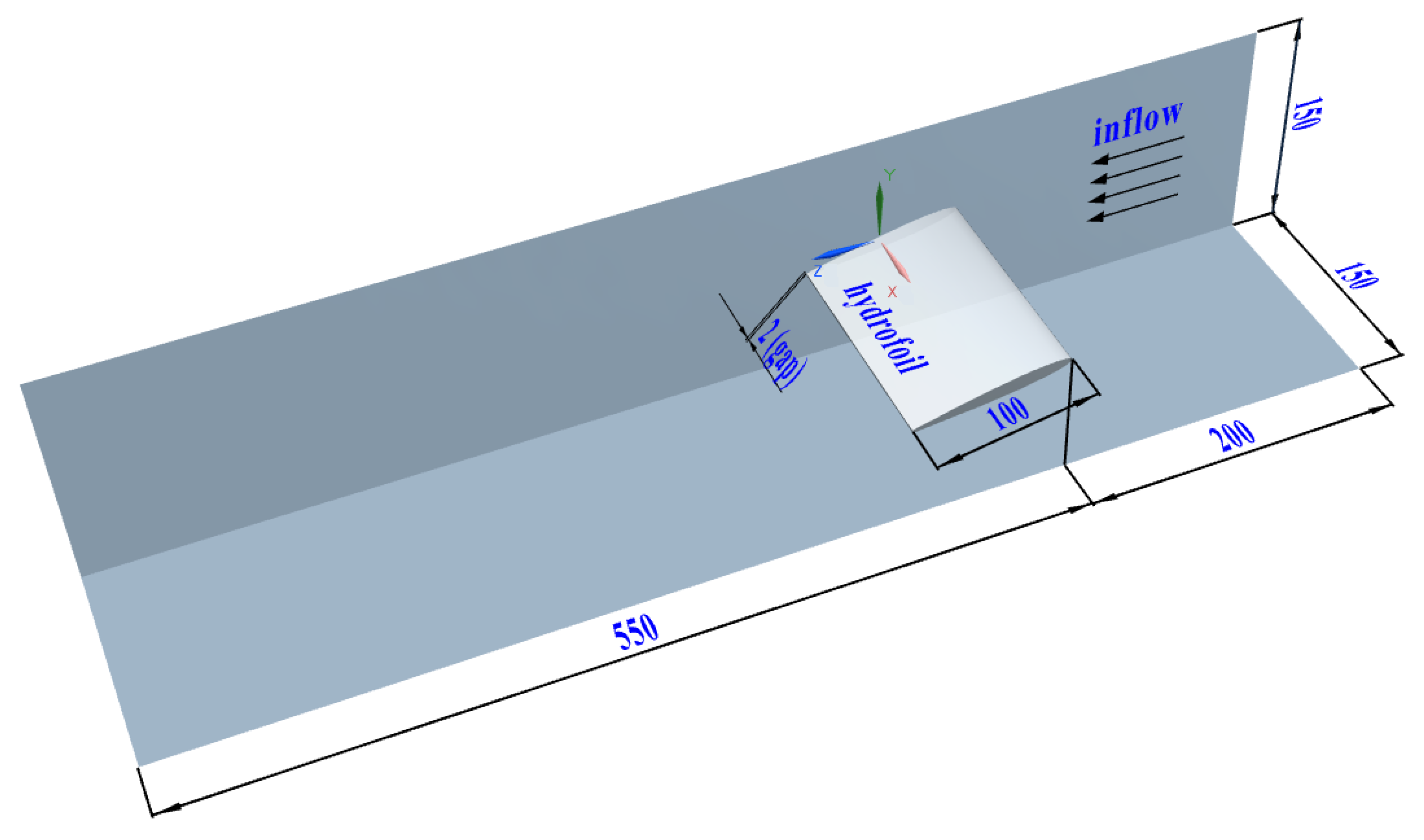
2.3. Hydrofoil Model and Setup

The present study focuses on a NACA0009 hydrofoil with an original chord of c₀ = 110 mm and a span of 150 mm, following the experimental setup of Dreyer et al. [25]. In the experiment, the hydrofoil truncated at c = 100 mm was mounted on a sliding support allowing an adjustable clearance between 0 and 20 mm. In addition, five incidence angles (3°, 5°, 7°, 10°, 12°) were tested in combination with four inflow velocities (5, 10, 15, and 20 m/s). It should be noted that only one of the experimental configurations was carried out in the current LES research.

The flow configuration and the coordinate system are schematically shown in Figure 1. The computational domain, which extends two chords upstream from the leading edge and 4.5 chords downstream from the trailing edge, has dimensions of $L_x\times L_y\times L_z=7.5c\times 1.5c\times 1.5c$, in which the subscript x, y and z represent spanwise, pitchwise and streamwise coordinates, respectively. The other important physical parameters for this simulation are as follows: the blade span is s = 1.48c, the size of the tip gap is τ = 0.02c, and the incidence angle is 10°. The boundary conditions are specified according to the experimental setup, and the inflow velocity, which will be a reference velocity to normalize the velocity variables, is fixed at V_∞ = 10 m/s with a turbulent intensity set at 1%. The corresponding Reynolds number is 1,120,000 based on the chord (c) and the inflow velocity (V_∞). A uniform outlet pressure is specified as P_outlet = 1 bar, and the corresponding cavitation number is 1.93 computed by $\sigma =\left(P_{outlet}-P_v\right)/0.5{\rho }_l{V}_{\infty }^2$. A no-slip boundary condition is set for the hydrofoil surface, and wall conditions are set for the boundaries of the tunnel.

2.4. Grid Spacing and Resolution

The mesh size is of extreme importance to ensure the validity of the LES computation because the LES approach filters the equations of momentum and decomposition of the flow variables into a large scale (resolved) and a small scale (unresolved) at the grid level. It is recommended that the mesh size in the region of primary interest should be located in the inertial subrange to resolve approximately 80% of the energy directly according to Pope’s theory [31]. Namely, the ratio of the grid size Δ to the lengthscale $l_{EI}$ should be less than 1.0, in which the lengthscale $l_{EI}$ is defined as the demarcation between the anisotropic large eddies ($l>l_{EI}$) and the isotropic small eddies ($l<l_{EI}$) according to Kolmogorov’s hypothesis. The distribution of $l_{EI}$ can be obtained by the following equations:

$$l_{EI}=\frac{1}{6}{L}_{11}$$

(12)

where $L_{11}$ is the integral length scale, and its ratio to the lengthscale of the energy-containing eddies ($L=k^{1.5}/\epsilon$) is a function of $R_{\lambda }$ as shown in Figure 2, and $R_{\lambda }$ is defined as:

$$R_{\lambda }={\left(\frac{20}{3}{\mathrm{Re}}_L\right)}^{1/2}={\left(\frac{20}{3}\frac{k^2}{\epsilon \upsilon }\right)}^{1/2}$$

(13)

where $R{e}_L$ is the turbulence Reynolds number defined by $R{e}_L=k^2/\epsilon \upsilon$, k is the local turbulent kinetic energy, $\epsilon$ is the local rate of turbulent energy dissipation, and $\upsilon$ is the kinematic viscosity.

To obtain the ratio of $\Delta /l_{EI}$, the spatial distribution of the lengthscale $l_{EI}$ or, equivalently, the distributions of total kinetic energy and dissipation are required. Consequently, before performing the LES, a RANS calculation should be carried out to determine the distributions of the kinetic energy and dissipation based on a relatively coarse mesh, which then serves as a guide for the mesh size in the region of primary interest. Then the LES is conducted with the modified mesh size until it satisfies the standard ($\Delta /l_{EI}\le 1$).

Based on the above method, and considering a compromise between calculation accuracy and computational time, the final ratio of the grid size $\Delta$ to the lengthscale l_EI is shown in a x-y plane at z/c = 0.3 where a variety of vortex structures are fully developed (Figure 3). This shows that the present LES is capable of resolving 80% of the energy at least in the region of primary interest (x/c < 0.1).

The mesh size used for the present study is 150 × 255 × 300. As shown in Figure 4, the meshes are clustered around the tip gap, blade pressure and suction surfaces, and end-wall to ensure appropriate resolution in the region of primary interest. There are 31 mesh points allocated across the tip-gap region for with a tip-gap size of 0.02c. Based on the chord in the spanwise, pitchwise, and streamwise directions, the grid spacings are $6.7\times {10}^{-4}\le \Delta x/c\le 5.5\times {10}^{-2}$, $5\times {10}^{-4}\le \Delta y/c\le 5\times {10}^{-2}$, and $5.8\times {10}^{-3}\le \Delta z/c\le 6.5\times {10}^{-2}$, respectively. The growth factor of the mesh around the tip-gap and blade surface is limited to a range of 1.0~1.2. The values of y⁺ varies due to different velocity magnitude, ranging from 0.3 to 19 with an average value of 3.4.

The LES was performed using commercial software ANSYS CFX. The time-dependent governing equations are discretized in both space and time domains and solved with a pressure-velocity coupling method using a finite volume method. A non-dissipative central-difference is used for spatial-discretization on a fine structure grid, which has been certified to be crucial for retaining the accuracy and predictive capability of the LES method [32,33,34]. For the transient terms, an implicit second-order Backward Euler scheme is used, which is recommended by ANSYS CFX. There are about 10 internal iterations to accomplish the convergence criterion (1 × 10⁻⁶) for a constant time step of 5 × 10⁻⁶ s. The corresponding non-dimensional time step based on the inflow velocity and the minimum mesh size (5 × 10⁻⁵ m) is 1, which ensures an average Courand-Friedrichs-Lewy number less than 1.0. In addition, the initial condition is specified by interpolating the velocity profile extracted from the RANS computations.

3. Results and Discussion

3.1. Validation of the LES

To check whether the LES is able to capture the accurate flow information and analyze the tip leakage vortex structures and dynamics characteristics, the present LES was validated against the experimental data. It should be noted that the foil tip pressure side corner was rounded with a small radius of 1mm in the experiment, which was not considered in the present LES.

Figure 5a shows the cavitation patterns in the whole computational domain defined by the vapor fraction iso-surface of α_v = 0.1 [22], and Figure 5b represents experimental cavitation patterns used to visualize the TLV trajectory. The qualitative comparison shows that the various cavitation patterns including the TLV cavitation, clearance cavitation and blade surface cavitation (behind in the TLV cavitation) in the experiment are also shown by the LES. However, the TLV cavitation appears almost along the whole chord in the experiment, while the iso-surface of vapor fraction only extends to 65% of the chord, which indicates that the TLV cavitation is underestimated by the present LES. On the contrary, the clearance cavitation predicted by the present LES is more intense than in the experiment. These differences are attributed to the influence of the rounded pressure edge which has an impact on the trajectory and the strength of the TLV [35], and contributes to reducing the clearance cavitation [36].

The quantitative comparisons between experimental data [37] and present LES results are presented in Figure 6, Figure 7 and Figure 8. Figure 6 shows the comparison of the TLV trajectories in the part of the flow field. Figure 7 shows the comparison of iso-lines of non-dimensional different streamwise vorticity calculated by ${\omega }_z^{*}=\left({\omega }_{z}c\right)/V_{\infty }$. Figure 8 shows the comparison of contours of each velocity component at x/c = 1.0.

As shown in Figure 6, the trajectories of TLV were generated by each vortex center defined as the point of maximum streamwise vorticity [18,37]. For the spanwise position (Figure 6a), the present computational TLV trajectory shows that TLV evolves closer to the endwall than the experiment. For the pitchwise position (Figure 6b), it is apparent that the trend of TLV evolution is well described by the present LES.

In Figure 7, it should be noted that the negative magnitude of streamwise vorticity predicted by present LES corresponds to the positive one in the experiment due to the opposite definition of streamwise direction. Figure 7a shows that the present computational results not only exhibit the profile of TLV fairly well, but also predict a high level of vorticity located around the TLV and near the endwall in the experiment. Figure 7b shows that the present LES can also predict the higher vorticity region well. Under both conditions, the iso-lines predicted by the present LES are quite reasonable in size and profile compared with the experimental measurements.

The top panel of Figure 8 shows that the whole magnitude of spanwise velocity ranging from the minimum to the maximum in the experiment is predicted better by the present LES. However, the pitchwise gradient of the spanwise velocity around the vortex center is spread on a larger band than that in the experiment. Similarly, the pitchwise velocity topology as shown in the middle panel of Figure 8 is again well captured by the present LES, while the spanwise gradient of the pitchwise velocity around the vortex center is not as steep as that in the experiment. Consequently, the strength of the TLV for the present LES is slightly weaker than that in the experiment. As for the streamwise velocity shown in the bottom panel of Figure 8, the velocity profile and the deficit of the streamwise velocity in the vortex center are captured well by the present simulation. However, the magnitude of the streamwise velocity of the hydrofoil wake viewed by on a horizontal region in the present LES is weaker than that in the experiment. Generally, the velocity topology and velocity magnitude predicted by the present computation agree better with the experimental data.

In summary, the present computational results accurately provide mean quantities and reach an adequate level of confidence to systematically analyze the characteristics of the TLV.

3.2. Development of Vortex Structures

In this section, mean streamlines were used to visualize the endwall vortex structures and investigate their development at different streamwise locations. To better understand the vortex structures in the endwall region, firstly a schematic was used to show the gross features, as shown in Figure 9. There are three main vortex structures: tip-leakage vortex which dominates the flow in the endwall region, tip separation vortex which is caused by flow separation, and induced vortex. To learn more about the generation and evolution of the endwall vortex structures observed in Figure 10a,c,e,g, the contour plots of the mean non-dimensional streamwise vorticity in the corresponding x-y planes are shown in Figure 10b,d,f,h, because the vorticity method makes it easier to clearly identify the vortex strength and its rotational direction which is generally difficult to recognize when only using mean streamlines.

As shown in Figure 10, vortex structures and their strength are completely different at different locations. At z/c = −0.4 (Figure 10a,e) which is close to the leading edge, the TLV is clearly captured with a compact structure near the suction side corner and rotates in counter-clockwise direction, and a tip separation vortex is underneath the hydrofoil rotating in the same direction as the TLV. There is also a small secondary vortex located slightly above the TLV near the suction surface, rotating in the opposite direction to the two other vortices, but its strength is relatively weak and it is not observed in any further downstream locations. At z/c = −0.1 (Figure 10c,d), the TLV is fully developed and its size increases substantially. Additionally, an induced vortex located in the lower-right of the TLV is displayed and rotates in clock-wise direction. At z/c = 0.2 (Figure 10e,f), the size of the TLV further increases and the core of the main part of the TLV is very well defined but less compact, and its strength is much reduced as displayed in Figure 10f. The induced vortex is no longer as clear as presented in Figure 10c and its strength also decreases suddenly. In addition, the TLV induces a swirling motion beyond its core causing the leakage flow to bend inward and then interact with the tip leakage jet, which generates an array of vortex filaments that rotate in the same direction as the TLV and extend from the suction tip edge to the TLV, as shown in Figure 10e,g. At z/c = 0.4 (Figure 10g,h), the TLV has lost its coherence and broken up, as shown in Figure 10h. The strength of the induced vortex is further reduced even though it is still well shown. Furthermore, there is no merging between the tip separation vortex and the TLV in this configuration.

Another remarkable feature is that the strength of the induced vortex decreases as the strength of the TLV decreases during the evolution of induced vortex (Figure 10c–h). This is because the formation of the induced vortex results from the interaction between the TLV and the wall boundary layer leading to the roll up of a part of the boundary layer [38]. Thus, the higher the strength of the TLV, the easier it is to roll up the boundary layer to form a strong induced vortex.

3.3. The Production Mechanism of Vorticity

Figure 11a,b illustrate the contour plots of the non-dimensional mean spanwise vorticity (${\omega }_z^{*}$) in x-y planes at two different streamwise locations (z/c = −0.1 and z/c = 0.2). Figure 11c,d show the pitchwise vorticity (${\omega }_y^{*}$) in corresponding planes. Compared with the corresponding streamwise vorticity shown in Figure 10b,d,f,g, it can be seen that the streamwise vorticity component dominates the vorticity field since the strength of streamwise vorticity of the TLV is much bigger than the two other vorticity components in the endwall region. Streamwise vorticity in the TLV is composed of two different velocity derivatives (ω_z = ∂v_y/∂x − ∂v_y/∂x), i.e., the spanwise derivatives of the pitchwise velocity (∂v_y/∂x) and the pitchwise derivatives of the spanwise velocity (∂v_y/∂x). However, it is mainly produced by the spanwise derivatives of the pitchwise velocity (${\omega }_z\approx \left(\partial v_y/\partial x\right)$) because the mean spanwise velocity is quite small.

Figure 12 shows the mean streamlines and the non-dimensional pitchwise velocity distributions in y-z planes close to the endwall (x/c = 0.01) and away from the endwall (x/c = 0.2). In Figure 12a, the flow undergoes a sudden change in the pressure side due to the existence of the pressure difference between the pressure side and the suction side, and eventually passes through the tip gap and converges. Because of the turning flow, a positive pitchwise velocity component is produced and its magnitude gradually reduces from the leading edge to the trailing edge in the tip leakage region as can be seen in the contour plot of pitchwise velocity in Figure 12a. While in the plane away from the end-wall (Figure 12b), the streamlines are approximately along the blade surface, and the magnitude of the pitchwise velocity is very small with no clear velocity gradient except in the leading edge region. The abrupt change of the pitchwise velocity along the blade span results in large spanwise derivatives of the mean pitchwise velocity (∂v_y/∂x), which plays a significant role in generating the strong vorticity of the TLV.

3.4. The TLV Development and Profile Evolution

In this section, some characteristics of the TLV were obtained by investigating the time averaged profiles of the pitchwise velocity and the axial velocity (i.e., streamwise velocity) along a horizontal line through the vortex core at different streamwise locations starting from the mid-chord to a downstream area far from the trailing edge.

Figure 13a shows the distribution of pitchwise velocity, in which the black crossed symbol represents the position of the vortex center. Note that the distance between the two maxima in these velocity profiles is indicative of the vortex core size [39]. This plot clearly shows that the two maxima of the pitchwise velocity decrease as the TLV moves downstream while the size of vortex core is increased monotonically, indicating that the vorticity in the vortex core gradually decreases from mid-chord to the area far away from the trailing edge according to the Rankine vortex model. Moreover, the positive maximum of the pitchwise velocity is larger than the absolute value of the maximum negative magnitude at any streamwise location (as clearly in shown in the middle panel of Figure 8 for z/c = 1.0), demonstrating that the velocity distribution in the core of the TLV is asymmetric. This can be explained by the image vortex with the same strength as the TLV rotating in the opposite direction required to satisfy the boundary conditions [40], and this image vortex induces a larger pitchwise velocity on the half of the actual vortex close to the endwall than that on the other half.

Figure 13b shows the axial velocity along the horizontal line. The axial flow in the vortex core features several interesting velocity profiles at different streamwise locations. At z/c = 0.0 the velocity in the vortex center is a jet-like profile with a peak velocity 23% higher than the inflow velocity, and in front of this location the velocity profile is also a jet-like region which is not depicted in this Figure At z/c = 0.1 the velocity around the vortex center approximates to the inflow velocity, while at z/c = 0.2 the axial velocity has a small velocity deficit with a value of 0.9V_∞ (wake-like profile) and the magnitude of this deficit further decreases to a value of about 0.5V_∞ as the TLV moves downstream to the streamwise location at z/c = 1.2. This progression (axial velocity profile in the vortex core changing from jet-like to wake-like) can be explained by the competition between the energy loss due to dissipation and the radial gradient in circulation strength according to Batchelor’s theory [41]. As discussed in Section 3.2, the TLV in front of the mid-chord has a more concentrated structure and a higher strength than that in the downstream area, so it produces a large radial gradient in circulation strength which generates a large axial velocity in the vortex center. Opposite to the region behind the mid-chord, the strength of the TLV gradually decreases but its radius increases further. This trend results in a small radial gradient compared with the location near the leading edge, and causes the interaction between the TLV and endwall boundary layer which intensifies the energy loss due to dissipation. As a result, a wake-like profile is produced. As the TLV moves further downstream from the trailing edge, the interaction with the hydrofoil wake leads to a further decrease in axial velocity in the vortex center. In addition, the streamwise velocity in the vortex center starts to increase behind the location at z/c = 1.2. This is because the strength of the TLV is quite small behind z/c = 1.2, it is not able to support its structure and starts to be assimilated by the surrounding flow and eventually dissipates due to the viscous influence.

4. Conclusions

In this paper, the characters of the tip leakage vortex was numerically investigated by LES, and the following conclusions can be derived based on the results obtained from this study:

(1)

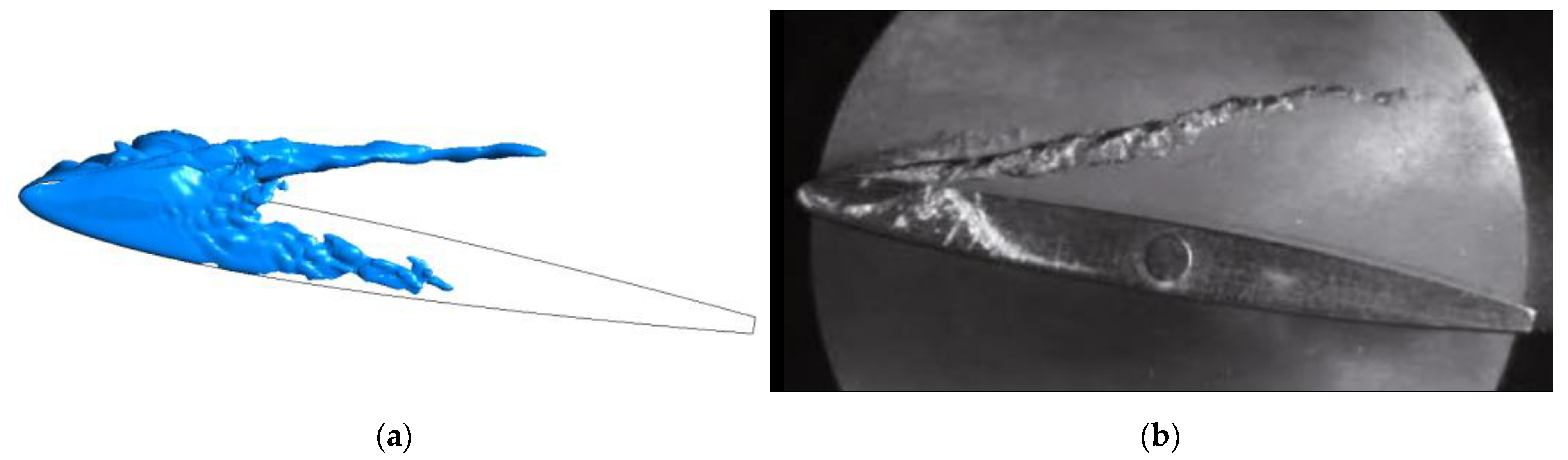
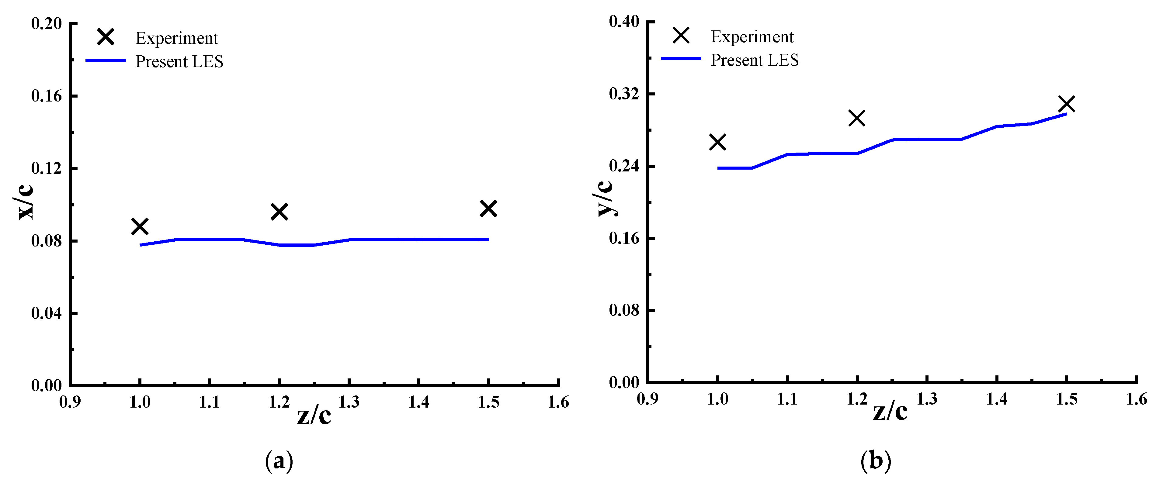
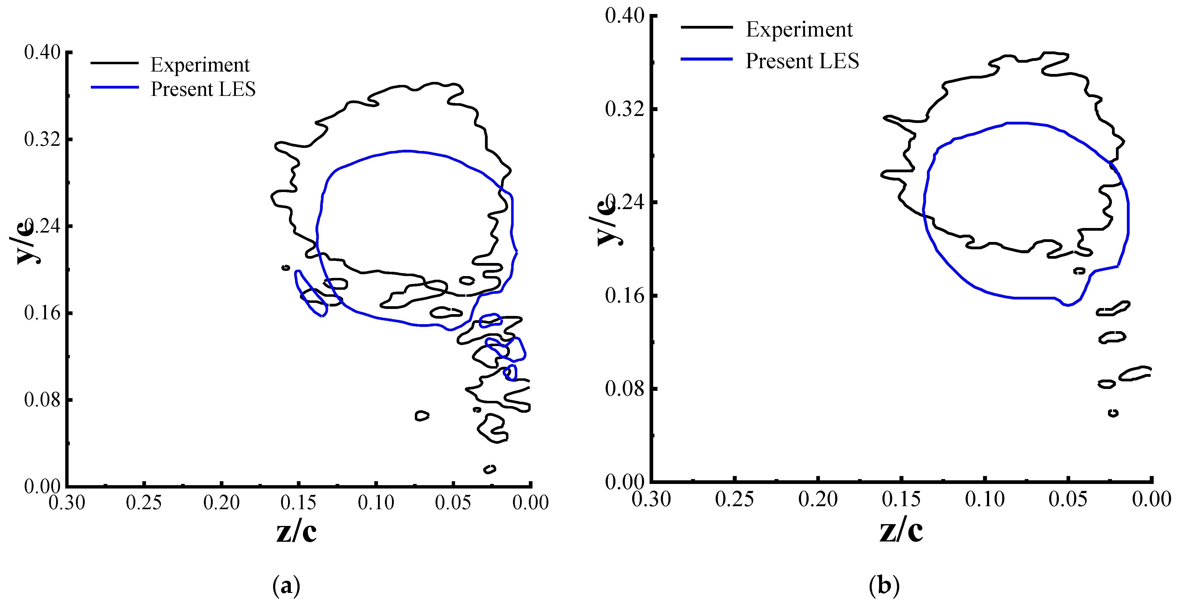
By validation of mesh sizes, the present LES predicts well the average characteristics of the TLV when compared to the experimental data.

(2)

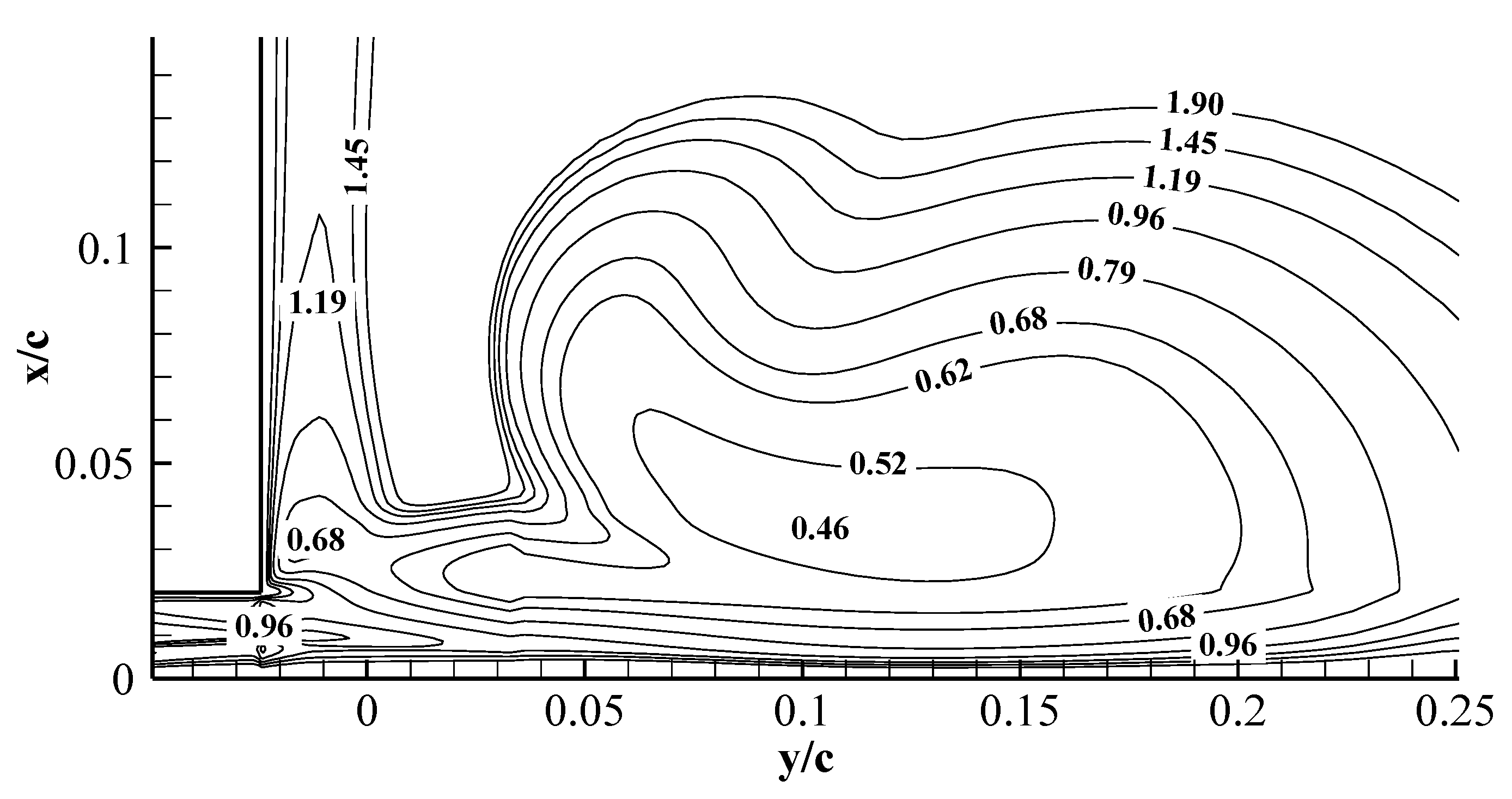
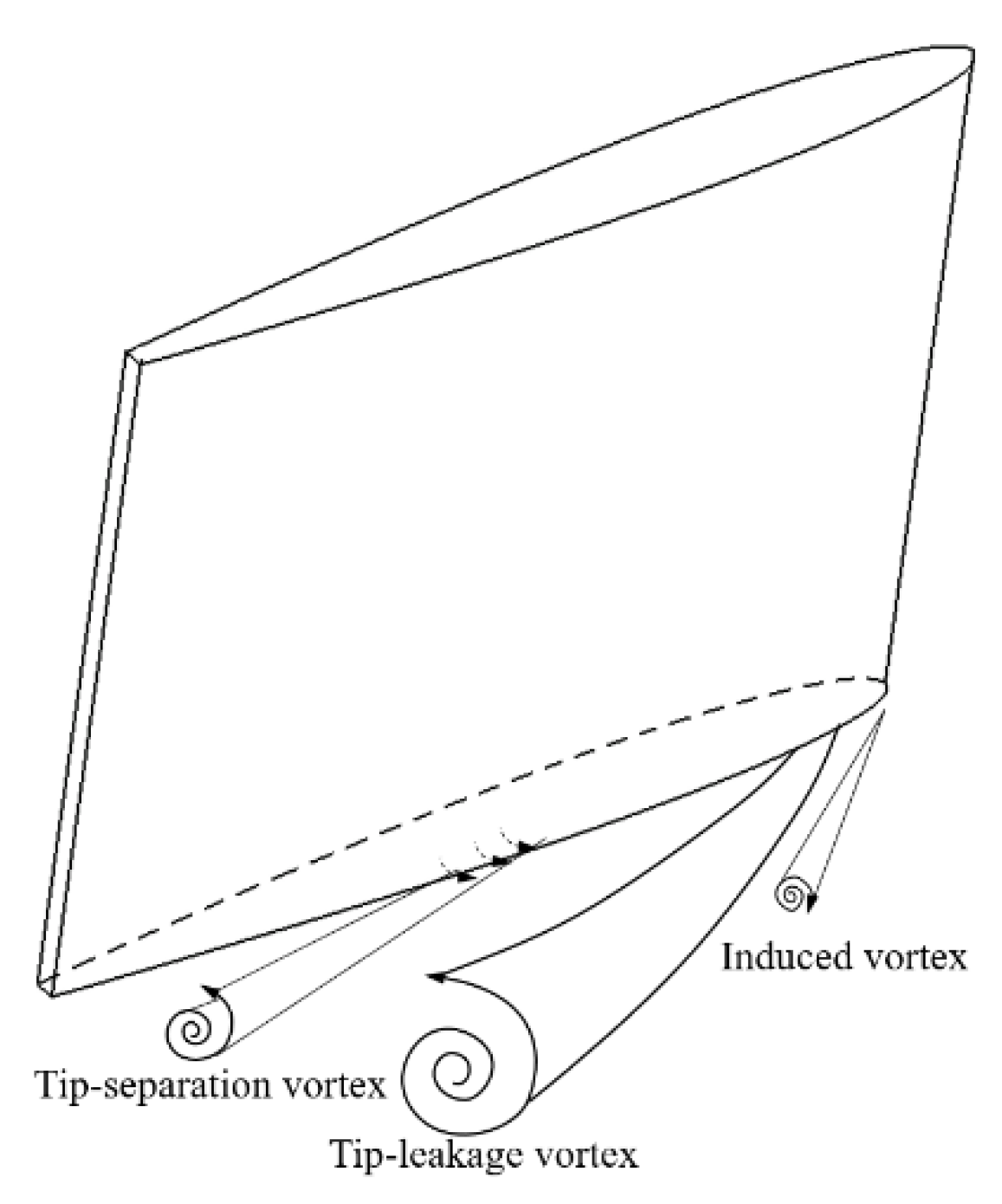
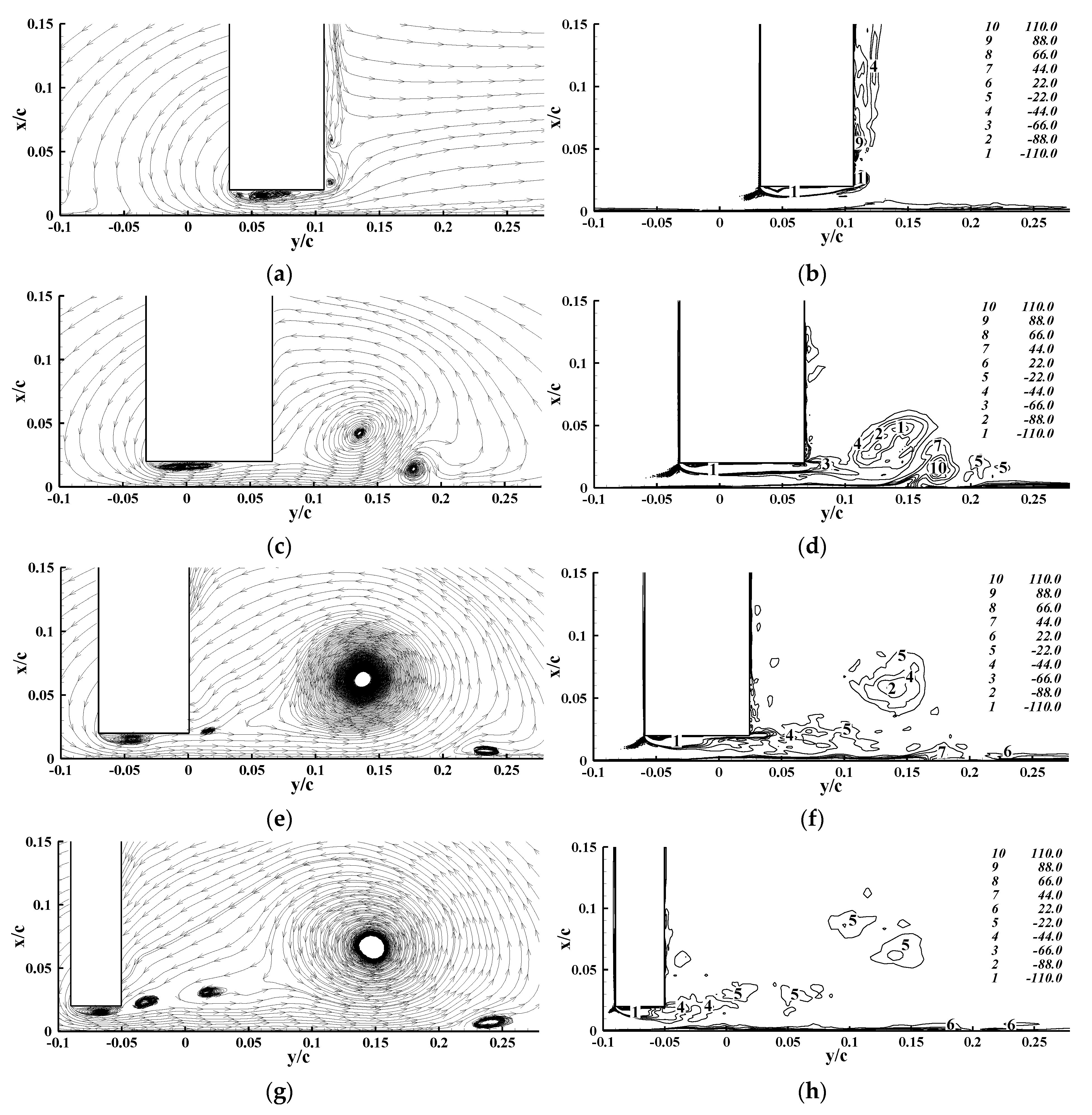
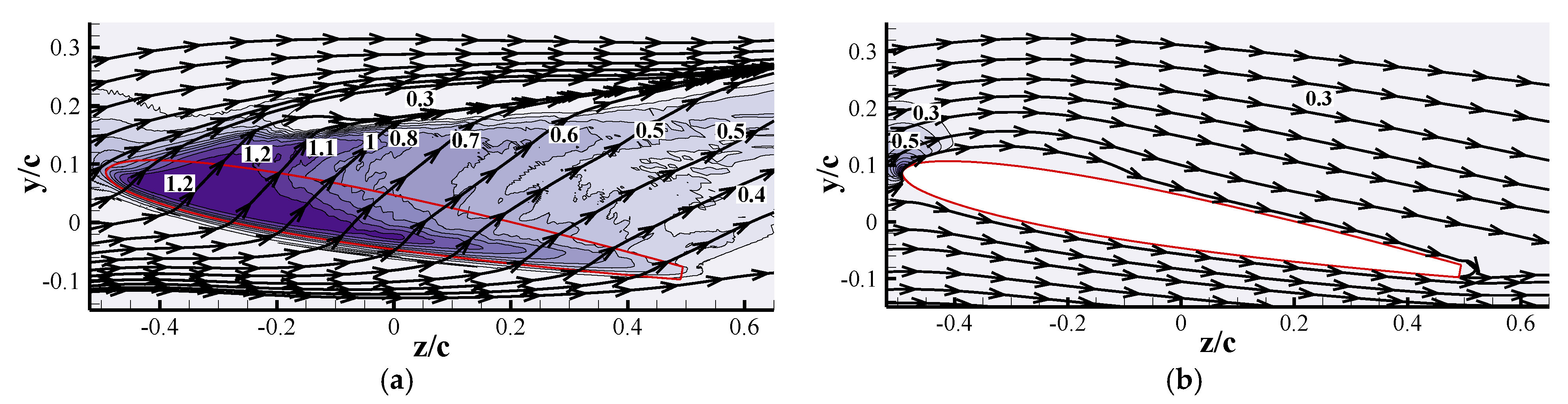
The various vortex structures in the endwall region are identified by the mean streamlines and the region of high non-dimensional streamwise vorticity. The TLV is found to dominate the endwall vortex structures.

(3)

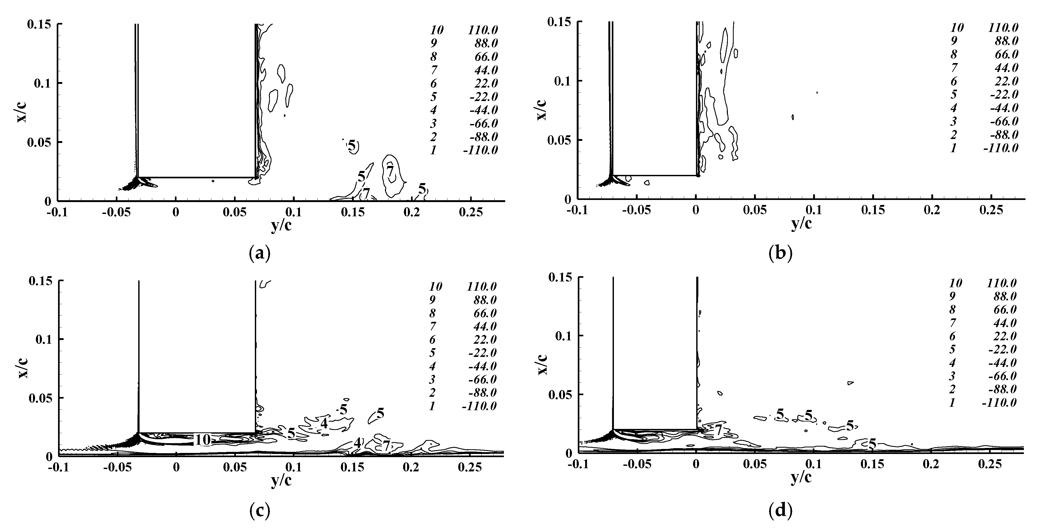
The streamwise vorticity component dominates the vorticity field compared to the different components of vorticity, and this streamwise vorticity component is mainly produced by the spanwise derivative of the mean pitchwise velocity.

(4)

During the TLV evolution, the vortex core radius keeps increasing, and its axial velocity experiences a switchover from a jet-like profile to a wake-like profile.

References

1. Denton, J.D. The 1993 IGTI Scholar Lecture: Loss Mechanisms in Turbomachines. J. Turbomach. 1993, 115, 621–656. [Google Scholar] [CrossRef]
2. Park, C.; Seol, H.; Kim, K.; Seong, W. A study on propeller noise source localization in a cavitation tunnel. Ocean Eng. 2009, 36, 754–762. [Google Scholar] [CrossRef]
3. Li, Y.S.; Cumpsty, N.A. Mixing in Axial Flow Compressors: Part I—Test Facilities and Measurements in a Four-Stage Compressor. J. Turbomach. 1991, 113, 161–165. [Google Scholar] [CrossRef]
4. Li, Y.S.; Cumpsty, N.A. Mixing in Axial Flow Compressors: Part II—Measurements in a Single Stage Compressor and a Duct. J. Mech. Des. 1990, 113, 166–174. [Google Scholar] [CrossRef] [Green Version]
5. Mailach, R.; Lehmann, I.; Vogeler, K. Rotating Instabilities in an Axial Compressor Originating From the Fluctuating Blade Tip Vortex. J. Turbomach. 2000, 123, 453–460. [Google Scholar] [CrossRef]
6. Rains, D.A. Tip Clearance Flows in Axial Compressors and Pumps. Ph.D. Thesis, California Institute of Technology, Pasadena, CA, USA, 2001. [Google Scholar]
7. Lakshminarayana, B.; Pouagare, M.; Davino, R. Three-Dimensional Flow Field in the Tip Region of a Compressor Rotor Passage—Part I: Mean Velocity Profiles and Annulus Wall Boundary Layer. J. Eng. Power 1982, 104, 760–771. [Google Scholar] [CrossRef]
8. Lakshminarayana, B.; Davino, R.; Pouagare, M. Three-Dimensional Flow Field in the Tip Region of a Compressor Rotor Passage—Part II: Turbulence Properties. J. Eng. Power 1982, 104, 772–781. [Google Scholar] [CrossRef]
9. Storer, J.A.; Cumpsty, N.A. Tip Leakage Flow in Axial Compressors. J. Turbomach. 1991, 113, 252–259. [Google Scholar] [CrossRef]
10. Kang, S.; Hirsch, C. Experimental Study on the Three-Dimensional Flow within a Compressor Cascade with Tip Clearance: Part I—Velocity and Pressure Fields. J. Turbomach. 1993, 115, 435–443. [Google Scholar] [CrossRef]
11. Kang, S.; Hirsch, C. Experimental Study on the Three Dimensional Flow within a Compressor Cascade with Tip Clearance: Part II—The Tip Leakage Vortex. J. Turbomach. 1992, 115, 444–452. [Google Scholar] [CrossRef]
12. Kang, S.; Hirsch, C. Tip Leakage Flow in Linear Compressor Cascade. J. Turbomach. 1994, 116, 657–664. [Google Scholar] [CrossRef]
13. Wu, H.; Miorini, R.L.; Katz, J. Measurements of the TLV structures and turbulence in the meridional plane of an axial water-jet pump. Exp. Fluids 2011, 50, 989–1003. [Google Scholar] [CrossRef]
14. Wu, H.; Tan, D.; Miorini, R.L.; Katz, J. Three-dimensional flow structures and associated turbulence in the tip region of a water-jet pump rotor blade. Exp. Fluids 2011, 51, 1721–1737. [Google Scholar] [CrossRef]
15. Wu, H.; Miorini, R.L.; Tan, D.; Katz, J. Turbulence within the Tip-Leakage Vortex of an Axial Waterjet Pump. AIAA J. 2012, 50, 2574–2587. [Google Scholar] [CrossRef]
16. Storer, J.A.; Cumpsty, N.A. An approximate analysis and prediction method for tip clearance loss in axial compressors. J. Turbomach. 1993, 116, 648–656. [Google Scholar] [CrossRef]
17. Shin, S. Reynolds-Averaged Navier-Stokes Computation of Tip Clearance Flow in a Compressor Cascade Using an Unstructured Grid. Ph.D. Thesis, Virginia Polytechnic Institute and State University, Blacksburg, VA, USA, 2001. [Google Scholar]
18. You, D.; Wang, M.; Moin, P.; Mittal, R. Effects of tip-gap size on the tip-leakage flow in a turbomachinery cascade. Phys. Fluids 2006, 18, 105102. [Google Scholar] [CrossRef] [Green Version]
19. You, D.; Wang, M.; Moin, P.; Mittal, R. Large-eddy simulation analysis of mechanisms for viscous losses in a turbomachinery tip-clearance flow. J. Fluid Mech. 2007, 586, 177–204. [Google Scholar] [CrossRef] [Green Version]
20. Gaggero, S.; Tani, G.; Viviani, M.; Conti, F. A study on the numerical prediction of propellers cavitating tip vortex. Ocean Eng. 2014, 92, 137–161. [Google Scholar] [CrossRef]
21. Zhang, D.; Shi, W.; van Esch, B.B.; Shi, L.; Dubuisson, M. Numerical and experimental investigation of TLV trajectory and dynamics in an axial flow pump. Comput. Fluids 2015, 112, 61–71. [Google Scholar] [CrossRef]
22. Zhang, D.; Shi, L.; Shi, W.; Zhao, R.; Wang, H.; Esch, B.P.M.V. Numerical analysis of unsteady TLV cavitation cloud and unstable suction-side-perpendicular cavitating vortices in an axial flow pump. Int. J. Multiph. Flow 2015, 77, 244–259. [Google Scholar] [CrossRef]
23. Higashi, S.; Yoshida, Y.; Tsujimoto, Y. Tip leakage vortex cavitation from the tip clearance of a single hydrofoil. JSME Int. J. 2002, 45, 662–671. [Google Scholar] [CrossRef] [Green Version]
24. Murayama, M. Unsteady tip leakage vortex cavitation originating from the tip clearance of an oscillating hydrofoil. J. Fluids Eng. 2006, 128, 421–429. [Google Scholar] [CrossRef]
25. Dreyer, M. Mind The Gap: Tip Leakage Vortex Dynamics and Cavitation in Axial Turbines. Ph.D. Thesis, EPFL, Lausanne, Switzerland, 2015. [Google Scholar]
26. Zwart, P.J.; Gerber, A.G.; Belamri, T. A two-phase flow model for predicting cavitation dynamics. In Proceedings of the Fifth International Conference on Multiphase Flow, Yokohama, Japan, 30 May–4 June 2004; Volume 152. [Google Scholar]
27. Mejri, I.; Bakir, F.; Rey, R.; Belamri, T.; Mejri, I. Comparison of computational results obtained from a homogeneous cavitation model with experimental investigations of three inducers. J. Fluids Eng. 2006, 128, 1308–1323. [Google Scholar] [CrossRef]
28. Luo, X.; Ji, B.; Peng, X.; Xu, H.; Nishi, M. Numerical simulation of cavity shedding from a three-dimensional twisted hydrofoil and induced pressure fluctuation by large-eddy simulation. J. Fluids Eng. 2012, 134, 041202. [Google Scholar] [CrossRef]
29. Germano, M.; Piomelli, U.; Moin, P.; Cabot, W.H. A dynamic subgrid-scale eddy viscosity model. Phys. Fluids A Fluid Dyn. 1991, 3, 1760–1765. [Google Scholar] [CrossRef] [Green Version]
30. Lilly, D.K. A proposed modification of the germano subgrid-scale closure method. Phys. Fluids A Fluid Dyn. 1992, 4, 633–635. [Google Scholar] [CrossRef]
31. Pope, S.B. Turbulent flows. Turbul. Flows 2001, 10, 806. [Google Scholar] [CrossRef]
32. Beaudan, P.; Moin, P. Numerical Experiments on the Flow Past a Circular Cylinder at Sub-Critical Reynolds Number (No. TF-62). Ph.D. Thesis, Stanford University, Stanford, CA, USA, 1995. [Google Scholar]
33. Mittal, R.; Moin, P. Suitability of upwind-biased finite difference schemes for large-eddy simulation of turbulent flows. AIAA J. 1997, 35, 1415–1417. [Google Scholar] [CrossRef]
34. You, D.; Mittal, R.; Moin, P.; Wang, M. Computational methodology for large-eddy simulation of tip-clearance flows. AIAA J. 2004, 42, 271–279. [Google Scholar] [CrossRef]
35. Lee, T.; Pereira, J. Nature of wakelike and jetlike axial tip vortex flows. J. Aircr. 2010, 47, 1946–1954. [Google Scholar] [CrossRef]
36. Laborde, R.; Chantrel, P.; Mory, M. Tip clearance and tip vortex cavitation in an axial flow pump. J. Fluids Eng. 1997, 119, 680–685. [Google Scholar] [CrossRef]
37. Decaix, J.; Balarac, G.; Dreyer, M.; Farhat, M.; Munch, C. RANS and LES computations of the tip-leakage vortex for different gap widths. J. Turbul. 2015, 16, 309–341. [Google Scholar] [CrossRef]
38. Doligalski, T.L.; Smith, C.R.; Walker, J.D.A. Vortex interactions with walls. Annu. Rev. Fluid Mech. 1994, 26, 573–616. [Google Scholar] [CrossRef]
39. Ghias, R.; Mittal, R.; Dong, H.; Lund, T. Study of tip-vortex formation using large-eddy simulation. AIAA J. 2005, 1280, 1–13. [Google Scholar]
40. Chen, G.T.; Greitzer, E.M.; Tan, C.S.; Marble, F.E. Similarity analysis of compressor tip clearance flow structure. J. Turbomach. 1991, 113, 260–271. [Google Scholar] [CrossRef]
41. Anderson, E.A.; Lawton, T.A. Correlation between Vortex Strength and Axial Velocity in a Trailing Vortex. J. Aircr. 2003, 40, 699–704. [Google Scholar] [CrossRef]
Figure 1. Computational domain with Cartesian coordinates.
Jmse 09 01198 g001
Figure 2. The ratio of the integral lengthscale L11 to L as a function of the Reynolds number for the model spectrum.
Jmse 09 01198 g002
Figure 3. The ratio of the grid size Δ to the lengthscale lEI at at z/c = 0.3.
Jmse 09 01198 g003
Figure 4. Meshing computational domain: (a) global mesh, and (b) local region A.
Jmse 09 01198 g004
Figure 5. Qualitative comparison of cavitation patterns: (a) vapor fraction iso-surface of αv = 0.1 predicted by the present LES, and (b) cavitation in the experiment.
Jmse 09 01198 g005
Figure 6. Comparison of trajectories of TLV: (a) spanwise, and (b) pitchwise.
Jmse 09 01198 g006
Figure 7. Comparison of iso-lines of the non-dimensional streamwise vorticity: (a)   ω z * = 2 , and (b)   ω z * = 3 .
Jmse 09 01198 g007
Figure 8. Comparison of contours of velocity components at x/c = 1.0: top: vx, middle: vy, and bottom: vz. (a) Present LES. (b) Experiment.
Jmse 09 01198 g008
Figure 9. Illustration of the flow structures in the endwall region.
Jmse 09 01198 g009
Figure 10. Mean streamlines and the corresponding contours of non-dimensional mean streamwise vorticity in x-y planes: (a,b) for z/c = −0.4, (c,d) for z/c = −0.1, (e,f) for z/c = 0.2, and (g,h) for z/c = 0.4.
Jmse 09 01198 g010
Figure 11. Contours of non-dimensional mean spanwise (top) and pitchwise (bottom) vorticity components in x-y planes: (a,c) for z/c = −0.1, and (b,d) for z/c = 0.2.
Jmse 09 01198 g011
Figure 12. Pitchwise velocity distributions normalized by the inflow velocity and the streamlines in y-z planes: (a) x/c = 0.01, and (b) x/c = 0.2.
Jmse 09 01198 g012
Figure 13. Distribution of velocity component along a horizontal line through vortex core: (a) Pitchwise velocity, and (b) axial velocity.
Jmse 09 01198 g013
Publisher’s Note: MDPI stays neutral with regard to jurisdictional claims in published maps and institutional affiliations.