Integral Sliding Mode Based Finite-Time Tracking Control for Underactuated Surface Vessels with External Disturbances

Abstract

This study focuses on the problem of finite-time tracking control for underactuated surface vessels (USVs) through sliding-mode control algorithms with external disturbances. Considering the nonexistence of relative degree caused by the underactuated property, the initial tracking error system is firstly transformed to a high order system for the possibility of applying a sliding-mode control algorithm. Subsequently, a finite-time controller based on an integral sliding surface (ISMS) is designed to achieve trajectory tracking. With the aid of this controller, the tracking errors converge to a steady state in a finite time. In contrast to the backstepping-based approach, the proposed method makes it possible to integrate controller design of position tracking and attitude tracking in one step, thus ensuring simplicity for implementation. Finally, theoretical analysis and numerical simulations are conducted to confirm the effectiveness of the proposed method.

1. Introduction

Over the past decades, USVs have attracted a continuously growing interest from the academic community attributing to its broad ocean application prospects, such as inspection, surveillance, and oceanography study, etc. For these missions, trajectory tracking control technologies are of great significance, especially when the harsh ocean environment is taken into consideration. Nevertheless, the ever-increasing complexity of marine environment and automation pose a variety of challenges for tracking a controller design of USVs. To guarantee desirable tracking performances, researchers have put forward a great diversity of control algorithms for USVs, involving prescribed performance control [1,2,3], backstepping control [4,5,6], and sliding-mode control [7,8,9]. Specifically, sliding-mode control has become a current research hotspot due to its robustness to external disturbances, model uncertainties, and system parametric variations.

A majority of the current literature concentrates on endowing fully actuated surface vessels with attractive properties, such as collision avoidance capability [10], excellent anti-saturation capability [11,12,13], and anti-interference [14]. A practical adaptive sliding-mode control scheme is proposed in [11] for an unmanned surface vehicle. Meanwhile, the auxiliary dynamic system and the adaptive technology are employed to handle input saturation and unknown disturbances, respectively. However, the above method can only achieve asymptotic stability, which makes the unmanned surface vehicles unable to face time-required maritime missions. Different from the basic sliding-mode control method used in [11]. In [13], subject to input saturations and unknown disturbances, finite-time trajectory tracking control of an unmanned surface vehicle is addressed by integral sliding-mode control and homogeneous disturbance observer as a technical extension of this result. Ref. [14] proposes a fixed-time sliding-mode control scheme for the rapid and accurate trajectory tracking of a fully actuated unmanned surface vehicles in the presence of model uncertainties and external disturbances. For the sake of fast converge speed for tracking missions, finite-time stability [14,15,16] and fixed-time stability [17,18,19] were ensured based on a sliding-mode control algorithm.

In spite of the effectiveness of these achievements for fully actuated vehicles, there is still the requirement to design controllers for USVs, especially in terms of the integration design. More specially, USVs’ controller design for position tracking and attitude tracking should be integrated together to provide simplicity in real implementations. Unfortunately, this kind of integration design is scarce, attributing to the USVs’ inherent underacted dynamics. The majority of current methods always divide USVs into two subsystems, i.e., surge motion and yaw motion. However, at present, various control algorithms focus on satisfying the steady-state performance of the system, and pay less attention to the transient performance (mainly refer to overshoot and convergence speed) [20,21,22]. In order to maintain control accuracy and provide satisfactions on transient performance for USVs, prescribed performance strategies have acquired extensive attention in both trajectory tracking issues [21,22] and cooperative formation issues [23,24,25]. Besides prescribed performance guarantees, communication frequency among different modules is another important criterion that deserves further investigation. To improve the applicability of tracking controllers and save onboard resources, the event-triggered mechanisms that could reduce data transmission rate were recently adopted for issues of dynamic positioning [25,26] and trajectory tracking [27,28]. Among these algorithms, it can only realize the asymptotic stability of the control system, which is not conducive to engineering applications with time requirements.

Inspired by these observations, it is essential but challenging to propose a proper strategy that can render the integration design a solvable issue for USVs. With this in mind, this paper is dedicated to designing an integrated finite-time algorithm for the tracking issues of USVs based on ISMS. The main contributions of this paper are shown as follows:

(i) As opposed to the backstepping based algorithms [20,21,22,23,24,25,26,27,28], the integration controller design for position motion and attitude motion is achievable with the employment of a novel model transformation method. Thus, it provides the feasibility for the actual marine application of the underactuated surface vessels. Consequently, the presented method enjoys a distinguishing feature of conciseness and simplicity for real implementation in the future.

(ii) Unlike current finite-time control algorithm [6,18,27], this paper constructs an artful ISMS, even if the initial error dynamics are transformed into a third-order system, the design of the integrated controller can still be realized, and the tracking errors have finite-time stability. Additionally, the devised updating laws will force the tracking errors converging to zero rather than a small region.

The rest of this paper is given as follows. In Section 2, the system model of underactuated ship is established and the control objective is set. Model transformation and adaptive controller is conducted in Section 3. Simulations are presented to validate the effectiveness of controller in Section 4. Finally, conclusions are obtained in Section 5.

2. System Dynamics and Problem Formulation

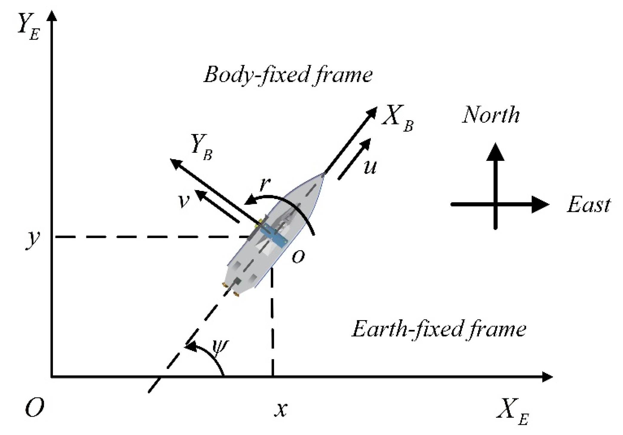
2.1. Modeling of USV

In this section, it is reasonable to assume that the desired trajectory of the USVs is described in the horizontal plane. Two coordinate systems, including the body-fixed coordinate $O_B{X}_B{Y}_B$ and the earth-fixed coordinate $O_E{X}_E{Y}_E$, are defined in Figure 1 to demonstrate the motions of USVs. By resorting to these two coordinates, the kinematic and dynamic mathematical models are constructed as (1) [29]:

$$\{\begin{array}{l}\dot{x}=u\cos \psi -v\sin \psi \\ \dot{y}=u\sin \psi +v\cos \psi \\ \dot{\psi }=r\end{array}$$

(1)

In which state variables $x$, $y$ and $\psi$ are defined under the coordinate $O_E{X}_E{Y}_E$. $x$, $y$, and $\psi$ represent USV’s position and the yaw angle. u, $v$, and $r$ denote the surge velocity, sway velocity, and yaw velocity with respect to $O_B{X}_B{Y}_B$, respectively.

$$\{\begin{array}{l}\dot{u}=(m_{22}vr-d_{11}u+{\tau }_u+{\tau }_{ud})/m_{11}\\ \dot{v}=(-m_{11}ur-d_{22}v)/m_{22}\\ \dot{r}=\left[(m_{11}-m_{22})uv-d_{33}r+{\tau }_r+{\tau }_{rd}\right]/m_{33}\end{array}$$

(2)

where $m_{ii},i=1,2,3$ represent inertia masses of ship, and $d_{ii},i=1,2,3$ denote the hydrodynamic coefficients. ${\tau }_u$ and ${\tau }_r$ are the control inputs which are generated by actuators. ${\tau }_{ud}$ and ${\tau }_{rd}$ denote the unknown time-varying disturbance caused by waves, winds, and ocean currents.

Remark 1.

It should be noted that only two control inputs, τ_u and τ_r, are involved in system Equations (1) and (2) with an exception in the sway channel, making the model underactuated of USVs. With only surge force and yaw moment available, the difficulty lies in how to eliminate the lateral position errors since sway channel is uncontrollable, which makes it a challenging work to design controllers for USVs.

Remark 2.

Since the design of lateral thruster is not only costly, but also causes hull hydrodynamic performance deterioration in high-speed scenarios, the USV platforms are often designed to be underactuated. As a result, only the propulsion force and yaw moment are necessary for most marine missions, which means that the investigations in this work are meaningful and practical.

2.2. Notations, Lemmas and Assumptions

The following assumptions and lemmas are given to facilitate the controller construction and model transformation.

Notations. 

In this paper, $\xi$ is a vector defined as $\xi ={\left[{\xi }_1,{\xi }_2,\dots ,{\xi }_n\right]}^{\mathrm{T}}$.The Euclidean norm and the determinants of matrix $\xi$ are defined as $\Vert \xi \Vert$ and $\det (\xi )$, respectively. Additionally, $\mathrm{sig}{(\xi )}^{\alpha }$ is defined as $\mathrm{sig}{(\xi )}^{\alpha }={\left[\mathrm{sign}({\xi }_1){\left|{\xi }_1\right|}^{\alpha },\mathrm{sign}({\xi }_2){\left|{\xi }_2\right|}^{\alpha }\right]}^{\mathrm{T}}$.

Lemma 1

([19]). For the system presented in Equations (1) and (2), if the Lyapunov function $V(\xi ):U\to R$ exists and satisfies:

$$\dot{V}(\xi )\le -\beta V{(\xi )}^{\gamma },\xi \in U_0\backslash \left\{0\right\}$$

(3)

with $\beta >0$, $0<\gamma <1$, and $U_0$ represent an open neighborhood containing the equilibrium point. Then, it can be concluded that $\xi =0$ is achieved in finite time T with $T\le \frac{V{(0)}^{1-\gamma }}{\beta (1-\gamma )}$.

Lemma 2

([20]). If a system satisfies the following equation:

$$\{\begin{array}{l}{\dot{\epsilon }}_1={\epsilon }_2\\ {\dot{\epsilon }}_2={\epsilon }_3\\ ⋮\\ {\dot{\epsilon }}_n=u\end{array}$$

(4)

And the controller is established as Equation (5) with ${\epsilon }_i,i=1,2,\dots ,n$:

$$u=-k_1\mathrm{sign}({\epsilon }_1){\left|{\epsilon }_1\right|}^{{\alpha }_1}-k_2\mathrm{sign}({\epsilon }_2){\left|{\epsilon }_2\right|}^{{\alpha }_2}-k_3\mathrm{sign}({\epsilon }_3){\left|{\epsilon }_3\right|}^{{\alpha }_3}-\cdots -k_n\mathrm{sign}({\epsilon }_n){\left|{\epsilon }_n\right|}^{{\alpha }_n}$$

(5)

It jumps to the conclusion that the system mentioned above possesses the character of finite-time convergence, where ${\alpha }_{j-1}=\frac{{\alpha }_j{\alpha }_{j+1}}{2{\alpha }_{j+1}-{\alpha }_j}$, $j=2,3,\dots ,n$ with ${\alpha }_n=\alpha$, ${\alpha }_{n+1}=1$, $\alpha \in (1-\iota ,1)$, $\iota \in (0,1)$. Moreover, $k_1,\dots k_n$ must ensure that $s^n+k_n{s}^{n-1}+\dots +k_1=0$ is Hurwitz.

Assumption 1.

During the tracking missions for USVs, the surge velocityuis supposed to be nonzero since the environment drift force and actuator torque always exist.

Assumption 2.

It assumes that there is always the inequation$m_{11}\ne m_{22}$for the inertial masses.

Assumption 3.

For the external disturbances${\tau }_{rd}$,${\dot{\tau }}_{ud}$,and${\tau }_{ud}$, inequalities$\left|{\dot{\tau }}_{ud}\right|\le D_1$,$\left|{\tau }_{rd}\right|\le D_2$and$\left|{\tau }_{ud}\right|\le D_3$exist, in which$D_1$,$D_2$,and$D_3$are positive constants. Then, a constant$D$is defined as$D=\sqrt{D_1^2+D_2^2}$.

Remark 3.

The inertia masses of USVs are composed of platform displacementmand added mass$\Delta m_{ii}$,$i=1,2,3$, which can be expressed as$m_{ii}=m+\Delta m_{ii}$. The added mass is mainly determined by the hull shape and motion direction as it is an inherent hydrodynamic characteristic in the fluid environments. Hence, Assumption 2 is tenable with the existence of the equation$\Delta m_{11}\ne \Delta m_{22}$for marine vehicles.

Remark 4.

In the ocean environment, external disturbances are always inscrutable, time-varying but bounded. In this case, the relation in Assumption 3 is deemed to be reasonable.

Control objective: 

This study is dedicated to proposing an integrated controller for the trajectory tracking task of USVs in the presence of external disturbances, enabling finite time stability of the tracking errors.

The following part is organized to complete this objective with the employment of the integral sliding-mode surface and Lyapunov-based analysis.

3. Controller Design

Due to the nonexistence of relative degree in USV systems, model transformation is first carried out in this section, which will transform the initial system to a high-order system. For the transformed system, the traditional finite-time sliding-mode control algorithm is no longer effective. To this end, the construction of a novel ISMS is presented with the combination of Lemma 2, which will make the tracking errors characterize with finite-time stability [30]. For the purpose of endowing the system with desirable adaptions to the complex environment, an adaptive updating law is established with adjustable design parameters.

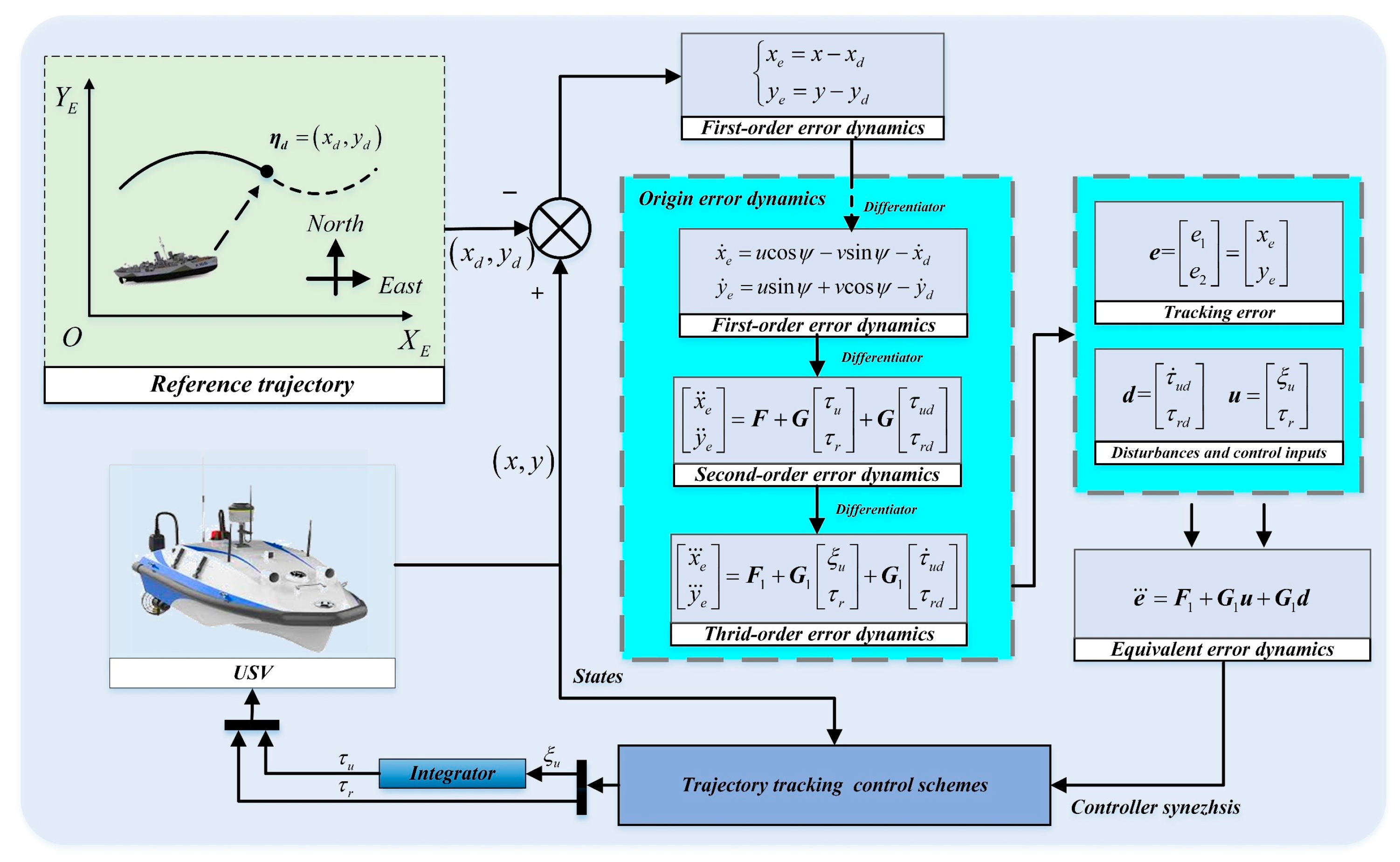
3.1. Model Transformation

On account of the underactuated property, it poses a great challenge to apply sliding-mode methods for USVs’ controller development, especially in tracking missions. However, due to the advantages of the sliding-mode control algorithm that can avoid complex calculations, it is necessary to develop the controller of underactuated surface vessels based on the sliding-mode surface. In order to solve this problem, the initial tracking error dynamics will be properly transformed to a 3-order system. The main architecture of the transformation process is shown in Figure 2.

By defining the reference trajectory as ${\eta }_d=(x_d,y_d)$, the tracking errors are derived as the following equation:

$$\{\begin{array}{l}{x}_e=x-x_d\\ y_e=y-y_d\end{array}$$

(6)

Based on the aforementioned preliminaries, the tracking issue in this study can be regarded as forcing the tracking errors converging to equilibrium point within finite time. To show the influence of under-actuation, the time derivative on both sides of Equation (6) is presented as:

$$\begin{array}{l}{\dot{x}}_e=u\cos \psi -v\sin \psi -{\dot{x}}_d\\ {\dot{y}}_e=u\sin \psi +v\cos \psi -{\dot{y}}_d\end{array}$$

(7)

Noting that the control inputs τ_u and τ_r do not appear on the right side of Equation (7), the further differentiation of Equation (7) is needed, thus leading to:

$$\begin{array}{l}{\ddot{x}}_e=\dot{u}\cos \psi -u\dot{\psi }\sin \psi -\dot{v}\sin \psi -v\dot{\psi }\cos \psi -{\ddot{x}}_d\\ {\ddot{y}}_e=\dot{u}\sin \psi +v\dot{\psi }\cos \psi +\dot{v}\cos \psi -v\dot{\psi }\sin \psi -{\ddot{y}}_d\end{array}$$

(8)

Then, Equation (8) is further developed as follows for better illustration:

$$\left[\begin{array}{c}{\ddot{x}}_e\\ {\ddot{y}}_e\end{array}\right]=F+G\left[\begin{array}{c}{\tau }_u\\ {\tau }_r\end{array}\right]+G\left[\begin{array}{c}{\tau }_{ud}\\ {\tau }_{rd}\end{array}\right]$$

(9)

$$F=\left[\begin{array}{c}{f}_u\cos \psi -ur\sin \psi -\dot{v}\sin \psi -vr\cos \psi -{\ddot{x}}_d\\ f_u\sin \psi +ur\cos \psi +\dot{v}\cos \psi -vr\sin \psi -{\ddot{y}}_d\end{array}\right]$$

(10)

$$G=\left[\begin{array}{cc}\cos \psi /m_{11}& 0\\ \sin \psi /m_{11}& 0\end{array}\right]$$

(11)

where $f_u=(m_{22}vr-d_{11}u)/m_{11}$, $f_r=\left[(m_{11}-m_{22})uv-d_{33}r\right]/m_{33}$.

As shown in Equation (11), it can be deduced that G is singular with $\det (G)=0$. Because of the invalid $G^{-1}$, synthesizing the controller directly based on Equation (9) is impossible for designers. To circumvent this, an alternative solution in existing work is to transmit origin error dynamics into a new combined system with a yaw guidance law [23]. For instance, a new position error and yaw error are constructed as ${\rho }_e=\sqrt{x_e^2+y_e^2}$ and ${\psi }_e=\mathrm{atan}2(x_e,y_e)$, respectively. However, singularity is not eliminated when ${\rho }_e=0$ or ${\psi }_e=\pm \frac{\pi }{2}$, though $y_e$ could be controlled in this way according to the analysis in [23]. Thus, finding alternatives to prevent this phenomenon from happening is imperative.

By viewing the control inputs τ_u and τ_r as state variables, further differential is taken on both sides of Equation (9) to achieve the relative degree of y_e:

$$\begin{array}{l}{\stackrel{⃛}{x}}_e=(\ddot{u}-\dot{v}\dot{\psi }-v\ddot{\psi })\cos \psi -(\dot{u}-v\dot{\psi })\dot{\psi }\sin \psi \\ -(\ddot{v}-\dot{u}\dot{\psi }-u\ddot{\psi })\sin \psi -(\dot{v}+u\dot{\psi })\dot{\psi }\cos \psi -{\stackrel{⃛}{x}}_d\\ {\stackrel{⃛}{y}}_e=(\ddot{u}-\dot{v}\dot{\psi }-v\ddot{\psi })\sin \psi +(\dot{u}-v\dot{\psi })\dot{\psi }\cos \psi \\ +(\ddot{v}+\dot{u}\dot{\psi }+u\ddot{\psi })\cos \psi -(\dot{v}+u\dot{\psi })\dot{\psi }\sin \psi -{\stackrel{⃛}{y}}_d\end{array}$$

(12)

By defining ${\dot{\tau }}_u={\xi }_u$, $\ddot{u}$ and $\ddot{v}$ can be rewritten as:

$$\begin{array}{l}\ddot{u}=(m_{22}\dot{v}r+m_{22}v\dot{r}-d_{11}\dot{u}+{\xi }_u+{\dot{\tau }}_{ud})/m_{11}\\ \ddot{v}=(-m_{11}\dot{u}r-m_{11}u\dot{r}-d_{22}\dot{v})/m_{22}\end{array}$$

(13)

For the sake of convenience, the following auxiliary variables are defined:

$$\begin{array}{l}{a}_u=(m_{22}\dot{v}r+m_{22}v{f}_r-d_{11}\dot{u})/m_{11}\\ b_u=m_{22}v/m_{11}{m}_{33}\\ a_v=(-m_{11}\dot{u}r-m_{11}u{f}_r-d_{22}\dot{v})/m_{22}\\ b_v=-m_{11}u/m_{22}{m}_{33}\end{array}$$

(14)

Consequently, Equation (13) can be further developed as the following expression:

$$\begin{array}{l}\ddot{u}=a_u+({\xi }_u+{\dot{\tau }}_{ud})/m_{11}+b_u({\tau }_r+{\tau }_{rd})\\ \ddot{v}=a_v+b_v({\tau }_r+{\tau }_{rd})\end{array}$$

(15)

Substituting Equation (15) into Equation (12), the following 3-order system can be obtained:

$$\left[\begin{array}{c}{\stackrel{⃛}{x}}_e\\ {\stackrel{⃛}{y}}_e\end{array}\right]=F_1+G_1\left[\begin{array}{c}{\xi }_u\\ {\tau }_r\end{array}\right]+G_1\left[\begin{array}{c}{\dot{\tau }}_{ud}\\ {\tau }_{rd}\end{array}\right]$$

(16)

where the intact expressions of $F_1$, $G_1$ are given as follows:

$$\begin{array}{l}{F}_1=\left[\begin{array}{c}(a_u-2\dot{v}r-v{f}_r-u{r}^2)\cos \psi -(a_v+2\dot{u}r-u{f}_r-v{r}^2)sin\psi -{\stackrel{⃛}{x}}_d\\ (a_u-2\dot{v}r-v{f}_r-u{r}^2)sin\psi +(a_v+2\dot{u}r-u{f}_r-v{r}^2)\cos \psi -{\stackrel{⃛}{y}}_d\end{array}\right]\\ G_1=\left[\begin{array}{cc}\cos \psi /m_{11}& ((m_{22}/m_{11}-1)v\cos \psi +(m_{11}/m_{22}-1)usin\psi )/m_{33}\\ \sin \psi /m_{11}& ((m_{22}/m_{11}-1)vsin\psi -(m_{11}/m_{22}-1)u\cos \psi )/m_{33}\end{array}\right]\end{array}$$

(17)

For simplification in the subsequent steps, $F_1$ and $G_1$ are presented as $F_1=\left[\begin{array}{c}{f}_{11}\\ f_{21}\end{array}\right]$ and $G_1=\left[\begin{array}{cc}{g}_{11}& g_{12}\\ g_{21}& g_{22}\end{array}\right]$.

Then, for the control coefficient matrix $G_1$ presented in Equation (17), it can be verified that:

$$\det (G_1)=\frac{(m_{11}-m_{22})u}{m_{11}{m}_{22}{m}_{33}}$$

(18)

From the above discussion, we learned that $m_{11}\ne m_{22}$ and $u\ne 0$. According to Equation (18), one can deduce that $G_1$ is invertible. Eventually, a newer error dynamic equation is established as:

$$\stackrel{⃛}{e}=F_1+G_{1}u+G_{1}d$$

(19)

where $e=\left[\begin{array}{c}{e}_1\\ e_2\end{array}\right]=\left[\begin{array}{c}{x}_e\\ y_e\end{array}\right]$, $u=\left[\begin{array}{c}{\xi }_u\\ {\tau }_r\end{array}\right]$ and $d=\left[\begin{array}{c}{\dot{\tau }}_{ud}\\ {\tau }_{rd}\end{array}\right]$.

Remark 5.

For the transformed error dynamics Equation (19), controller design for surge motion and yaw motion could be integrated together, which is the main feature that distinguishes the proposal in this paper from the existing backstepping based control algorithms [20,21,22,23,24,25,26].

3.2. Adaptive Controller Design with External Disturbances

In this section, we will use the hyperbolic tangent function to design an adaptive controller to compensate for the external time-varying marine environment disturbances. The initial underactuated system is transformed to a 3-order system Equation (19), which is the foundation of the controller synthesis. However, it puts forward a new challenge to ensure finite-time convergence for this 3-order system. Taking this problem into account, an ISMS will be established such that desirable performance is obtained during tracking missions. The diagram of the tracking controller is depicted in Figure 3.

To facilitate the application of Lemma 2 for stability analysis, an ISMS is presented as the following expression:

$$s=(\ddot{e}-\ddot{e}(0))+{\displaystyle {\int }_{t_0}^t\left[k_1\mathrm{sig}{(e(l))}^{{\alpha }_1}+k_2\mathrm{sig}{(\dot{e}(l))}^{{\alpha }_2}+k_3\mathrm{sig}{(\ddot{e}(l))}^{{\alpha }_3}\right]}dl$$

(20)

where ${\alpha }_1=\frac{\alpha }{4-3\alpha }$, ${\alpha }_2=\frac{\alpha }{3-2\alpha }$, and ${\alpha }_3=\frac{\alpha }{2-\alpha }$ with $\alpha \in (1-\iota ,1)$, $\iota \in (0,1)$. In addition, $k_1$, $k_2$, and $k_3$ are provided to make sure $z^3+k_3{z}^2+k_{2}z+k_1=0$ is Hurwitz.

Remark 6.

According to Lemma 2,${\alpha }_j,j=2,3,4$is designed with${\alpha }_{j-1}=\frac{{\alpha }_j{\alpha }_{j+1}}{2{\alpha }_{j+1}-{\alpha }_j}$for the sake of possessing global finite-time convergence. Besides, tracking performance can be adjusted by just turning corresponding design parameters α, k₁, k₂and k₃.

Remark 7.

It is the state variables that are deemed to be far from the sliding manifold at the initial stage for general sliding-mode control methods. Additionally, during the reaching phase, systems possess much sensitivity to perturbances and parameter variations. In the proposed ISMS, these two disadvantages are well treated.

With the application of Equations (19) and (20), the derivative of s can be written as:

$$\begin{array}{ll}\dot{s}& =\stackrel{⃛}{e}+k_1\mathrm{sig}{(e(l))}^{{\alpha }_1}+k_2\mathrm{sig}{(\dot{e}(l))}^{{\alpha }_2}+k_3\mathrm{sig}{(\ddot{e}(l))}^{{\alpha }_3}\\ & =F_1+G_{1}u+G_{1}d+k_1\mathrm{sig}{(e(l))}^{{\alpha }_1}+k_2\mathrm{sig}{(\dot{e}(l))}^{{\alpha }_2}+k_3\mathrm{sig}{(\ddot{e}(l))}^{{\alpha }_3}\end{array}$$

(21)

Then, the tracking controller is synthesized as follows with ${\eta }_1>D$ and ${\eta }_2>0$:

$$u=-G_1^{-1}\left[k_1\mathrm{sig}{(e(l))}^{{\alpha }_1}+k_2\mathrm{sig}{(\dot{e}(l))}^{{\alpha }_2}+k_3\mathrm{sig}{(\ddot{e}(l))}^{{\alpha }_3}+F_1+{\eta }_{2}s\right]-{\eta }_1\mathrm{sign}(G_1^{\mathrm{T}}s)$$

(22)

Remark 8.

The two parameters, η₁and η₂, are designed to adjust the overshoot and convergence rate of s to some extent. More specifically, larger η₁and η₂mean larger overshoot and shorter settling time.${\alpha }_i,k_i,i=1,2,3$are control parameters that determine the performance of tracking errors when the sliding-mode surface is stabilized. In this account, the proper values of parameters should be selected based on the expected performance requirements.

Remark 9.

When the control scheme Equation (22) is constructed, it cannot be implemented for USVs directly since${\dot{\tau }}_u$rather than${\tau }_u$is designed here. Thus,${\tau }_u={\displaystyle {\int }_0^t{\xi }_u}dt$should be utilized for real applications.

Theorem 1.

For the USV system Equation (19) under Assumptions 1–3, the tracking of reference trajectories will be finished in finite time when the control scheme is designed as Equation (22) with the control parameters satisfying η₁ > D and η₂ > 0.

Proof of Theorem 1.

See Appendix A.1. □

Remark 10.

Summarizing the analysis given above, the integral sliding-mode manifold is constructed and the stability of the system is ensured by endowing the designed parameters with proper value under the circumstance of available D. For the feasibility in real applications, further research should be carried out for unavailable D.

Although the presented control algorithm Equation (22) provides effectiveness in tracking missions for USVs, it relies heavily on the information of external disturbances. However, it is impossible to acquire this kind of knowledge in marine engineering, which will cause much performance degradation or even makes this controller cease to be applicable. To this end, it makes sense to revisit the above tracking problem with an adaptive control scheme that is designed to obtain an estimation of external disturbances. On the basis of the analysis given above and recalling Equation (22), we redesign the control scheme and Equations (23) and (24) with γ₁, η₁, η₂, η₃ being positive constants and $\widehat{D}$ being the estimation of D:

$$\begin{array}{c}u=-G_1^{-1}[k_1\mathrm{sig}{(e(l))}^{{\alpha }_1}+k_2\mathrm{sig}{(\dot{e}(l))}^{{\alpha }_2}+k_3\mathrm{sig}{(\ddot{e}(l))}^{{\alpha }_3}\\ +F_1+{\eta }_1\mathrm{sign}(s)+{\eta }_{2}s]-{\eta }_3\mathrm{sign}(G_1^{\mathrm{T}}s)\tanh (\widehat{D})\end{array}$$

(23)

$$\dot{\widehat{D}}=\Vert s\Vert \Vert G_1\Vert \frac{{\gamma }_1}{{\eta }_3}{\cosh }^2(\widehat{D})$$

(24)

Remark 11.

For the purpose of disturbance rejection, the estimation parameter$\widehat{D}$is designed here. It is$\tanh (\widehat{D})$rather than$\widehat{D}$that is directly utilized in the control law (23). In this way, the designed adaptive law will lead to bounded control input even when it approaches infinite values.

Remark 12.

Under the existing algorithms for tracking missions of USVs, the controller can only guarantee asymptotical convergence, which means that the tracking errors will be constrained within a region as time goes infinite. In contrast to this situation, the presented proposal makes it possible to drive tracking errors shrinking to zero in finite time, thus improving tracking accuracy and convergence rate considerably.

Remark 13.

In consideration of the special definition of Equation (24), we define the estimation error as$\tilde{D}=D-{\eta }_3\tanh (\widehat{D})$to facilitate the stability analysis. Upon utilizing this definition, finite-time convergence of e is illustrated in what follows.

Theorem 2.

For the USV system Equation (19) under Assumptions 1–3, the desired trajectory will be followed within finite time if the control algorithm is implemented as Equations (23) and (24) with γ₁, η₁, η₂, η₃being positive constants. In addition,$\tilde{D}$will remain ultimately bounded.

Proof of Theorem 2.

See Appendix A.2. □

Remark 14.

Stability analysis of e is based on the combination of Lemma 1 and Lemma 2. By resorting to the newly defined estimation error$\tilde{D}=D-{\eta }_3\tanh (\widehat{D})$, this ISMS will be illustrated converging to zero under the constructed controller. Thus, tracking accuracy is considerably improved when it is compared with current researches [6,18,27]. In view of the presented analysis, it concludes that tracking accuracy and estimation accuracy are well guaranteed.

4. Simulation Results

In this section, two simulation examples are presented for manifesting the validity and superiority of the devised tracking controllers. Specifically, the first experiment was conducted to reveal the effectiveness and robustness of the proposed controller Equation (23) when the adopted USV underwent external disturbances. Aiming at further illustrating the preferable peculiarities of the proposed algorithm, the second experiment was conducted by comparing with the existing work [29] in the condition of different levels of parameter variations and disturbances. More details of the simulation results are exhibited in the subsequent part.

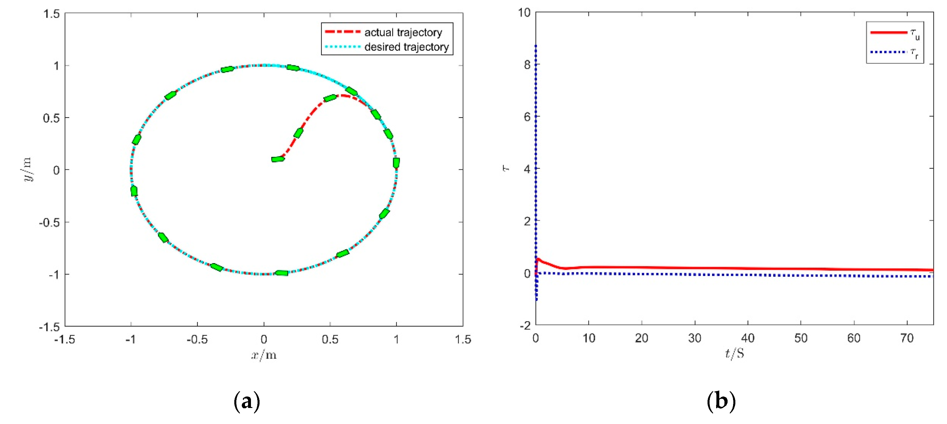
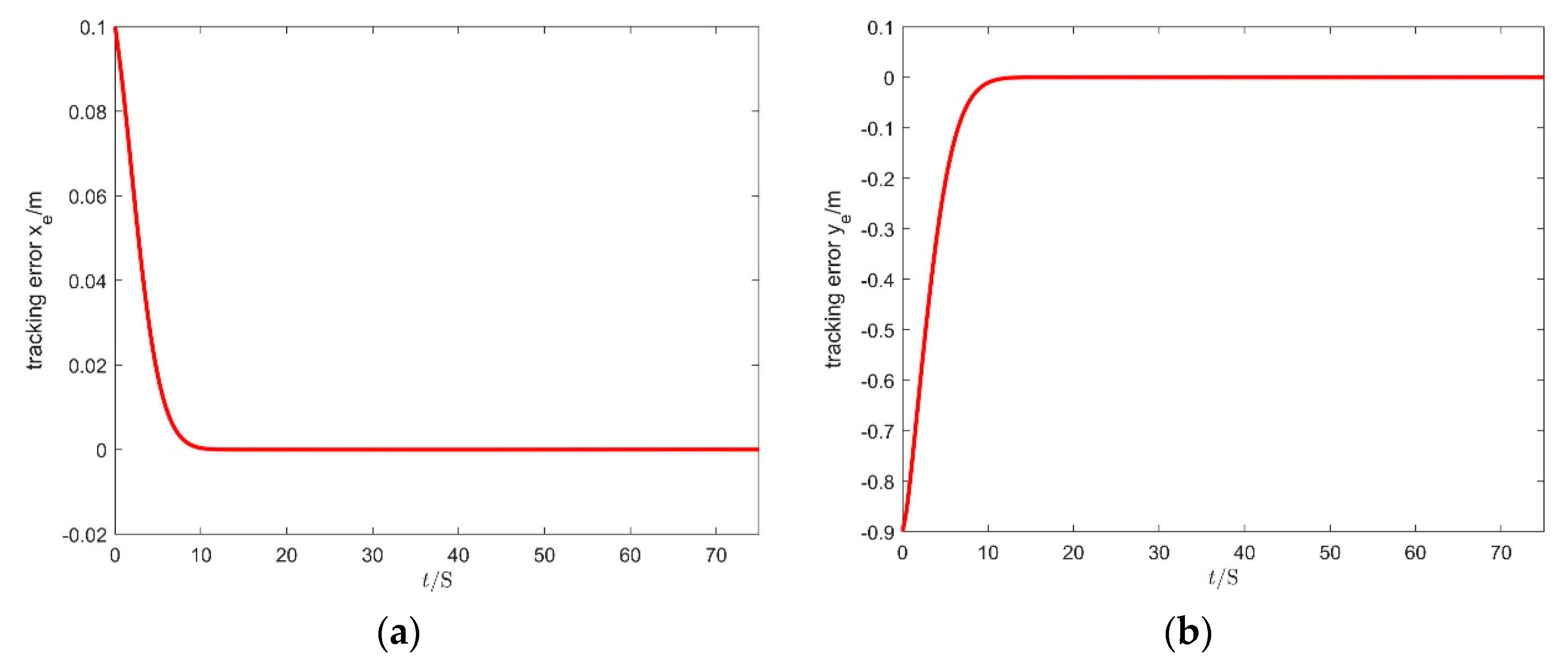
4.1. Simulation of ISMS Controller

Here, the motion dynamics of the USV are carried out by Equations (1) and (2). With the reference of [29], its model parameters could be given as

Table 1. Main parameters of USV.

Model Parameters	Values
[m11, m22, m33]T	[1.956, 2.405, 0.043]T (Unit: kg)
[d11, d22, d33]T	[2.436, 12.992, 0.0564]T

.

As stated in Remarks 6 and 8, the tracking error performance will be governed by the control parameters’ selection. Consequently, the parameters that appear in ISMS (20), as well as control laws (22) (23) and adaptive law (24), are properly chosen as

Table 2. Designed parameters of the control algorithm.

Control Parameters	Values
[k1, k2, k3]T	[1, 3, 3]T
[η1, η2, η3]T	[5, 5, 0.5]T
γ, α	0.05, 0.9

for trading off accuracy against convergence rate.

Without loss of generality, the initial states are set as $x(0)=0.1$, $y(0)=0.1$, $\psi (0)=0.1$, $u(0)=0.1$, $v(0)=0.1$, $r(0)=0.1$, and the desired trajectory is expressed as $(x_d,y_d)=(\sin (0.1t),\cos (0.1t))$. Besides, to imitate the variability of the marine environment more preferably, the external disturbances are taken as ${\tau }_{ud}={\tau }_{rd}=0.2\sin (0.01t)\mathrm{N}$.

As depicted in Figure 4a, the actual trajectory of USV can track the desired curve successfully in a timely manner. More detailed, the control inputs, as shown in Figure 4b, are of considerable changes at the initial stage so as to achieve a fast response. When the tracking errors turn to the stable state, there still exist the small control input signals producing to maintain the disturbance cancellation capability. For better observation of tracking precision, time responses for x_e and y_e are figured out in Figure 5. It is distinct that the tracking errors converge to zero within 10 s. It can be observed from Figure 6a that the uncontrolled state v keeps steady and increases slightly within an allowable range. Thus, the overall stability of this underactuated system can be achieved. From Figure 6b, the estimation value of perturbances increases fast at the initial phase for compensating the tracking errors. Though it always keeps increasing, the term $\tanh (\widehat{D})$ can ensure finite torques imposed on the USV system.

4.2. Comparative Simulation Results on the Different Conditions

In this subsection, the experiments consisting of two scenarios are conducted by comparing with the existing dynamic inverse controller Equation (14) in [29]. For brevity, the proposed controller in the paper is called ISMS, while the dynamics inverse controller in [29] is called as DI. With the unchanged model parameters and control parameters that shown in Table 1 and Table 2, simulation results of two specific circumstances are presented hereinafter.

Case 1. The model parameters of USV exhibited in Table 1 are suffering from 15% uncertainties and the external disturbances are chosen as ${\tau }_{ud}={\tau }_{rd}=0.3\sin (0.1t)\mathrm{N}$. The simulated wave surface of external disturbances in Case 1 is given in Figure 7.

Case 2. The model uncertainties are further enlarged to 25% and the external disturbances are set as ${\tau }_{ud}={\tau }_{rd}=0.6\sin (0.01t)\mathrm{N}$ to further show the excellent robustness of devised methods compared to the existing DI controller. The simulated wave surface of external disturbances in Case 2 is given in Figure 8.

The tracking error and control torques of Case 1 are presented in Figure 9 and Figure 10, while the corresponding results of Case 2 are presented in Figure 11 and Figure 12. It is observed from Figure 9 and Figure 11 that bigger perturbances and uncertainties will cause unexpected oscillations to tracking errors when the DI controller is applied. Totally different from this, satisfactory tracking performance will be remained under the presented controller in this paper. The tracking errors can converge to zero within 10 s without oscillation. As seen from Figure 10 and Figure 12, the output of controller DI changed a lot at the initial stage, which will lead to a significant hardware burden and even cause the occurrence of actuator faults. The ISMS control scheme has higher control accuracy. From these two aspects, one can deduce that the ISMS control scheme possesses the better convergence speed and control accuracy against disturbances and parameter variations. Therefore, it can be seen that, compared with the DI controller, the ISMS control scheme has better control performance.

5. Conclusions

The adaptive finite-time tracking control issue of USVs is tackled in the investigation with the employment of an integration design method. Firstly, the position motion and the attitude motion are treated as a whole in the design process, which mainly relies on a novel model transformation approach. Then, the finite-time controller of underactuated surface vessels is designed by using ISMS under external disturbances so that all signals of the closed-loop system converge to a stable state within a finite time. Additionally, control accuracy is improved to some extent due to the fact that tracking errors are forced to converge to zero instead of a small region when an artful adaptive updating law is devised. Finally, theoretical illustration and numerical simulations reflect the validity and appealing features of the presented methods. The advantage of the controller designed in this paper is that all control signals can converge in a finite time. Compared with the usual backstepping method, the calculation complexity is simplified and the differential explosion is avoided. The disadvantage is that the input saturation of the actuator is not considered. This will also be our direction in future research. In future work, we will study the underactuated surface vessels control considering both input saturation and actuator failure.

References

1. Dai, S.-L.; He, S.; Wang, M.; Yuan, C. Adaptive Neural Control of Underactuated Surface Vessels with Prescribed Performance Guarantees. IEEE Trans. Neural Netw. Learn. Syst. 2018, 30, 3686–3698. [Google Scholar] [CrossRef]
2. He, S.; Dai, S.-L.; Luo, F. Asymptotic Trajectory Tracking Control With Guaranteed Transient Behavior for MSV with Uncertain Dynamics and External Disturbances. IEEE Trans. Ind. Electron. 2018, 66, 3712–3720. [Google Scholar] [CrossRef]
3. Jia, Z.; Hu, Z.; Zhang, W. Adaptive output-feedback control with prescribed performance for trajectory tracking of underactuated surface vessels. ISA Trans. 2019, 95, 18–26. [Google Scholar] [CrossRef]
4. Lu, Y.; Zhang, G.; Sun, Z.; Zhang, W. Robust adaptive formation control of underactuated autonomous surface vessels based on MLP and DOB. Nonlinear Dyn. 2018, 94, 503–519. [Google Scholar] [CrossRef]
5. Qin, H.; Li, C.; Sun, Y.; Wang, N. Adaptive trajectory tracking algorithm of unmanned surface vessel based on anti-windup compensator with full-state constraints. Ocean Eng. 2020, 200, 106906. [Google Scholar] [CrossRef]
6. Qin, H.; Li, C.; Sun, Y.; Li, X.; Du, Y.; Deng, Z. Finite-time trajectory tracking control of unmanned surface vessel with error constraints and input saturations. J. Frankl. Inst. 2019, 357, 11472–11495. [Google Scholar] [CrossRef]
7. Zhang, P.; Guo, G. Fixed-time switching control of underactuated surface vessels with dead-zones: Global exponential stabilization. J. Frankl. Inst. 2020, 357, 11217–11241. [Google Scholar] [CrossRef]
8. Zhang, J.; Yu, S.; Yan, Y. Fixed-time velocity-free sliding mode tracking control for marine surface vessels with uncertainties and unknown actuator faults. Ocean Eng. 2020, 201, 107107. [Google Scholar] [CrossRef]
9. Weng, Y.; Wang, N.; Soares, C.G. Data-driven sideslip observer-based adaptive sliding-mode path-following control of underactuated marine vessels. Ocean Eng. 2020, 197, 106910. [Google Scholar] [CrossRef]
10. Mina, T.; Singh, Y.; Min, B.-C. Maneuvering Ability-Based Weighted Potential Field Framework for Multi-USV Navigation, Guidance, and Control. Mar. Technol. Soc. J. 2020, 54, 40–588. [Google Scholar] [CrossRef]
11. Qiu, B.; Wang, G.; Fan, Y.; Mu, D.; Sun, X. Adaptive sliding mode trajectory tracking control for unmanned surface vehicle with modeling uncertainties and input saturation. Appl. Sci. 2019, 9, 1240. [Google Scholar] [CrossRef] [Green Version]
12. Zhao, Y.; Sun, X.; Wang, G.; Fan, Y. Adaptive Backstepping Sliding Mode Tracking Control for Underactuated Unmanned Surface Vehicle With Disturbances and Input Saturation. IEEE Access 2020, 9, 1304–1312. [Google Scholar] [CrossRef]
13. Wang, N.; Gao, Y.; Shuailin, L.; Er, M.J. Integral sliding mode based finite-time trajectory tracking control of unmanned surface vehicles with input saturations. India J. Geo Mar. Sci. 2017, 46, 2493–2501. [Google Scholar]
14. Yao, Q. Fixed-time trajectory tracking control for unmanned surface vessels in the presence of model uncertainties and external disturbances. Int. J. Control 2020, 1–11. [Google Scholar] [CrossRef]
15. Yao, Q. Adaptive finite-time sliding mode control design for finite-time fault-tolerant trajectory tracking of marine vehicles with input saturation. J. Frankl. Inst. 2020, 357, 13593–13619. [Google Scholar] [CrossRef]
16. Yu, Y.; Guo, C.; Yu, H. Finite-Time PLOS-Based Integral Sliding-Mode Adaptive Neural Path Following for Unmanned Surface Vessels With Unknown Dynamics and Disturbances. IEEE Trans. Autom. Sci. Eng. 2019, 16, 1500–1511. [Google Scholar] [CrossRef]
17. Zhang, J.; Yu, S.; Yan, Y. Fixed-time output feedback trajectory tracking control of marine surface vessels subject to unknown external disturbances and uncertainties. ISA Trans. 2019, 93, 145–155. [Google Scholar] [CrossRef]
18. Zhou, B.; Huang, B.; Su, Y.; Zheng, Y.; Zheng, S. Fixed-time neural network trajectory tracking control for underactuated surface vessels. Ocean. Eng. 2021, 236, 109416. [Google Scholar] [CrossRef]
19. Zhang, J.X.; Yang, G.H. Fault-Tolerant Fixed-Time Trajectory Tracking Control of Autonomous Surface Vessels with Specified Accuracy. IEEE Trans. Ind. Electron. 2019, 67, 4889–4899. [Google Scholar] [CrossRef]
20. Lu, Y.; Zhang, G.; Qiao, L.; Zhang, W. Adaptive output-feedback formation control for underactuated surface vessels. Int. J. Control. 2018, 93, 400–409. [Google Scholar] [CrossRef]
21. Dai, S.L.; He, S.; Lin, H. Transverse function control with prescribed performance guarantees for underactuated marine surface vehicles. Int. J. Robust Nonlinear Control 2019, 29, 1577–1596. [Google Scholar] [CrossRef]
22. Wang, S.; Tuo, Y. Robust trajectory tracking control of underactuated surface vehicles with prescribed performance. Pol. Marit. Res. 2020. [Google Scholar] [CrossRef]
23. Yoo, S.J.; Park, B.S. Guaranteed performance design for distributed bounded containment control of networked uncertain underactuated surface vessels. J. Frankl. Inst. 2017, 354, 1584–1602. [Google Scholar] [CrossRef]
24. Park, B.S.; Yoo, S.J. An error transformation approach for connectivity-preserving and collision-avoiding formation tracking of networked uncertain underactuated surface vessels. IEEE Trans. Cybern. 2018, 49, 2955–2966. [Google Scholar] [CrossRef] [PubMed]
25. Zhang, G.; Yao, M.; Xu, J.; Zhang, W. Robust neural event-triggered control for dynamic positioning ships with actuator faults. Ocean Eng. 2020, 207, 107292. [Google Scholar] [CrossRef]
26. Liu, L.; Zhang, W.; Wang, D.; Peng, Z. Event-triggered extended state observers design for dynamic positioning vessels subject to unknown sea loads. Ocean Eng. 2020, 209, 107242. [Google Scholar] [CrossRef]
27. Deng, Y.; Zhang, X.; Im, N.; Zhang, G.L.; Zhang, Q. Model-based event-triggered tracking control of underactuated surface vessels with minimum learning parameters. IEEE Trans. Neural Netw. Learn. Syst. 2019, 31, 4001–4014. [Google Scholar] [CrossRef] [PubMed]
28. Ma, Y.; Nie, Z.; Yu, Y.; Hu, S.; Peng, Z. Event-triggered fuzzy control of networked nonlinear underactuated unmanned surface vehicle. Ocean Eng. 2020, 213, 107540. [Google Scholar] [CrossRef]
29. Ye, L.; Zong, Q. Tracking control of an underactuated ship by modified dynamic inversion. ISA Trans. 2018, 83, 100–106. [Google Scholar] [CrossRef] [PubMed]
30. Sun, H.; Li, S.; Sun, C. Finite time integral sliding mode control of hypersonic vehicles. Nonlinear Dyn. 2013, 73, 229–244. [Google Scholar] [CrossRef]
Figure 1. Coordinates definition of USV motioning in horizontal planes.
Jmse 09 01204 g001
Figure 2. The structure of the model transformation.
Jmse 09 01204 g002
Figure 3. Diagram of the tracking controller for USVs.
Jmse 09 01204 g003
Figure 4. Reference trajectory tracking in xy plane (a) and Control inputs (b).
Jmse 09 01204 g004
Figure 5. Time response of tracking errors regarding x-axis (a) and y-axis (b).
Jmse 09 01204 g005
Figure 6. Time response of uncontrolled state v (a) and the estimation variable D ^ (b).
Jmse 09 01204 g006
Figure 7. Wave surface of external disturbances in Case 1.
Jmse 09 01204 g007
Figure 8. Wave surface of external disturbances in Case 2.
Jmse 09 01204 g008
Figure 9. Comparative tracking errors of x-axis (a) and y-axis (b) under Case 1.
Jmse 09 01204 g009
Figure 10. Comparative control inputs τu (a) and τr (b) under Case 1.
Jmse 09 01204 g010
Figure 11. Comparative tracking errors of x-axis (a) and y-axis (b) under Case 2.
Jmse 09 01204 g011
Figure 12. Comparative control inputs τu (a) and τr (b) under Case 2.
Jmse 09 01204 g012