Abstract
In this study, we constructed a rapid refresh wave forecast model using sea winds from the Korea Local Analysis and Prediction System as input forcing data. The model evaluated the changes in forecast performance considering the influence of input wind–wave interaction, which is an important factor that determines forecast performance. The forecast performance was evaluated by comparing the forecast results of the wave model with the significant wave height, wave period, and wave direction provided by moored buoy observations. During the typhoon season, the model tended to underestimate the conditions, and the root mean square error (RMSE) was reduced by increasing the wind and wave interaction parameter. The best value of the interaction parameter that minimizes the RMSE was determined based on the results of the numerical experiments performed during the typhoon season. The forecast error in the typhoon season was higher than that observed in the analysis results of the non-typhoon season. This can be attributed to the variations of the wave energy caused by the relatively strong typhoon wind field considered in the wave model.
1. Introduction
Global, regional, local coastal, and regional probability wave forecast models currently used by the Korea Meteorological Administration (KMA) generate forecasts for sea weather conditions. Although these conditions vary constantly, the forecasts contribute significantly toward responding to extreme weather conditions and supporting safe maritime activities. However, accidents at sea and maritime disasters occur every year due to extreme weather despite using wave forecast systems. Moreover, the increase in various maritime activities has threatened the safety of the public. Therefore, providing wave forecast information for rapid response and countermeasure planning with regard to extreme weather is essential.
The wave forecast model currently operated was constructed based on WAVEWATCH3 (WW3), which is the standard wave forecast model used for wave research globally. Due to the presence of various physics modules, WW3 uses a model optimization process to execute highly accurate numerical modeling. It was configured to consider the effects of tide, current, sea ice, and other factors [1,2,3,4,5,6,7,8]. However, sensitivity experiments are required to select the appropriate physics modules and parameters because the WW3 model is highly sensitive to changes in the packages and variables [9,10,11]. Several studies investigated the effects of the physics packages in the wave model by implementing various physical phenomena in the model, such as wave–wave interactions, wind–wave interactions, wave energy dissipation, and wave breaking phenomena, considering the coastal topography [12,13,14,15,16,17,18,19]. Researchers have reported results regarding wave dispersion and nonlinear effects [20,21,22,23,24,25,26]. Furthermore, studies are actively being conducted to calculate the accuracy of atmospheric input fields, which is an important factor in determining the accuracy of forecast models [27,28,29,30,31]. In addition, research on the characteristics of wind waves developed by extreme wind fields, such as typhoons, is actively being conducted [32,33,34,35,36,37].
However, most of the aforementioned studies focus on physical phenomena that appear on a global scale, and research on wave models that incorporate the rapidly changing weather phenomena of local areas is limited. Analysis and prediction results are greatly affected by the physical modules and parameterizations of the wave model and the quality of the input wind field. Therefore, it is necessary to closely evaluate these impacts and construct the most suitable wave model [38,39,40].
In this study, we used the Korea Local Analysis and Prediction System (KLAPS) for the Korean Peninsula region to construct a rapid refresh wave forecast model, which incorporates the rapidly changing atmospheric conditions. Numerical experiments were performed under various conditions to examine the effect of the input wind and wave interaction on the results of the forecast model. The forecast results obtained for the typhoon season were compared with the observation data, and the effects of the input wind and wave interactions were evaluated under multiple experimental conditions. Based on the results, the forecast performance of the model was verified in terms of the significant wave height, wave period, and wave direction during the rapidly changing atmospheric conditions of the typhoon season.
2. Methodology
2.1. Model Setup and Observation Data
The proposed rapid refresh wave forecast model constructed based on WW3 was assigned a modeling area with a latitude of 32–44 N° and a longitude of 120–132 E°. The wind field forecast data for this area include the waters around the Korean Peninsula (Figure 1). The ETOPO1 global data from the National Geophysical Data Center (NGDC) were used for the ocean bathymetric grid, and Global Self-consistent, Hierarchical, High-resolution Shoreline (GSHHS) data were used to obtain the high-resolution shoreline data.
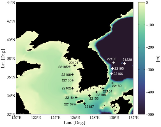
Figure 1.
Numerical domain and topography for the rapid refresh wave forecast model (+ indicates the ocean data buoys).
In order to perform the rapid wave forecast, the computational grids are evenly distributed (1/12° × 1/12° resolution) over the entire domain with a total number of 21,025 cells (145 × 145). The model uses 25 spectral frequency bins ranging from 0.0412 to 0.4056 Hz with a logarithmic increment factor of 1.1 and 36 directional bins with a resolution of 10 degrees. The wave forecast system is implemented with ST4 source packages. Equation (1) is for the wind input parameterization in ST4.
where is a wind–wave source term, is a growth parameter, is the effective wave age, is von Kármán constant, is the phase speed, is the wind friction velocity, and represents the spectral densities. In this way, the wind–wave source term contains parameterizations for the input wind field and directly affects the calculation of the wave spectral energy. In addition, since interactions between variables are included, step-by-step numerical simulation experiments should be performed according to variables in constructing sensitivity experiments [38].
To verify the forecast performance of the wave model, we used data that were observed at 30 min intervals using 16 ocean data buoys operated by the KMA. Figure 1 depicts the installation locations of the ocean data buoys. The observation data provide the significant wave height, marine weather observations on wave direction, wind speed, pressure, and other factors. As ocean data are provided in real time, it is extremely useful for rapidly ascertaining and responding to marine weather conditions.
2.2. Sea Wind Data
To generate rapid refresh wave forecast information, it is necessary to obtain the sea wind forecast results of an atmospheric model that can generate forecasts by reflecting rapidly changing atmospheric conditions. In this study, the 10 m sea wind forecast results of KLAPS, which performs forecasts at 1 h intervals for 12 h, served as the input wind field. Additionally, the wave model was set to perform forecasts every hour for 12 h considering the execution time and forecast time of the atmospheric model. The boundary conditions were obtained using the forecast results provided by a regional wave forecast model based on WW3, which was executed at 12 h intervals. The results that were forecast by running the model for 1 h prior to the execution formed the initial conditions of this study.
As the forecast results of the wave model are affected by the accuracy of the sea winds that are used as the input wind field, it is necessary to closely examine the wind–wave interaction growth parameter () as seen in Equation (1), which quantifies the direct effect of the input wind field on wave development [38,41,42,43]. Therefore, it plays a dominant role in the wave development and propagation processes and exhibits a more significant effect on the wave forecast results than other physical parameters. As this is the most dominant variable with respect to wind–wave development, a previous study examined the effect of changes in the physical variables of the rapid refresh wave model by varying the value of between 1.15 and 3.25, and the wave model was executed for the non-typhoon season [44].
Conversely, the forecast results for each experimental condition in this study were evaluated considering the typhoon season as seen in Table 1. These parameters in the wave model are important to determine the accuracy of the forecast performance because the wind–wave interaction growth parameter must be adjusted to different wind fields [11].

Table 1.
Numerical experimental conditions of wind–wave interaction growth parameter (Reproduced with permission from Roh et al., J. Korean Soc. Coast. Ocean Eng.; published by J. Korean Soc. Coast. Ocean Eng., 2020.) [44].
2.3. Verification Method
The experimental conditions for the aforementioned were applied, and the wave model was run from 00 UTC on 1 September 2019 to 23 UTC on 30 September 2019. Typhoons Lingling and Tapah, which occurred in September 2019, were modeled numerically. The rapid changes in the atmosphere due to the typhoons were the direct cause of large amounts of damage. Therefore, this period is considered the most suitable for evaluating the forecast performance of the proposed rapid refresh wave forecast model.
Figure 2 depicts the best track data of the typhoons provided by the Joint Typhoon Warning Center (JTWC). The results were compared with the observed significant wave heights based on the best track data collected during the same period, and the forecast performance was evaluated for each experimental condition.
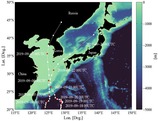
Figure 2.
Best tracks of Lingling (2–8 September 2019) and Tapah (19–23 September 2019) provided by the Joint Typhoon Warning Center (JTWC).
To evaluate the forecast performance of the wave model, the significant wave height, wave period, and wave direction results for the entire run time and all observation points of the wave model (Figure 1) were divided by the forecast time from +00 h to +12 h. Equations (2) and (3) were used to calculate the mean error (bias) and root mean square error (RMSE) using the observed values at all observation points, respectively [45].
where denotes the forecast value, indicates the observed value, and represents the weighting factor. The monthly forecast results for each experimental condition in terms of the significant wave height, wave period, and wave direction observed by the marine weather buoys were averaged for the run time of the entire model. Thus, the overall forecast performance of the wave model was evaluated by considering the forecast lead time from +00 h to +12 h. In addition to the significant wave height, the effects of changes in on the wave period and wave direction were analyzed using the same method.
3. Results
3.1. Verification of the Sea Wind Forecast Performance
Before evaluating the prediction performance of the wave model based on the changes in , we examined the sea winds as the input wind forcing data around the Korean Peninsula for one month. The analysis time was from 00 UTC on 1 September 2019 to 23 UTC on 30 September 2019. Table 2 lists the monthly averaged bias and RMSE of sea winds at all observation points for each forecast lead time calculated using Equations (1) and (3). The bias for each forecast lead time verifies that the model initially exhibited a tendency toward underestimation. However, the model tended to overestimate with the increase in the forecast lead time. The average RMSE for one month was approximately 2.5 m/s, and according to the forecast lead time, the difference was not large.
Table 2.
Values of bias and root mean square error (RMSE) of sea wind data averaged over all observation points.
In general, a high prediction performance is shown at the beginning of prediction time, whereas the prediction performance of the input wind field of KLAPS used in this study tended to decrease as the prediction time increased. This phenomenon is due to an optimization option that improves the predictive performance of the standby model. Therefore, to improve the forecast performance of the wave model, the effects of forecast error in the atmospheric model must be minimized. This implies that the effects of changes in input wind forcing and wave interactions need to be considered.
3.2. Results of the Numerical Experiments and Evaluation of the Effects of Wind–Wave Interaction Growth Parameter
To evaluate the effects of changes in , the forecast results for each experimental condition were divided considering the forecast time.
Figure 3 depicts the results of executing the Case00 wave model. Here, was 1.65, which served as the control case for the numerical experiment in this study. Figure 3a–c illustrate the time when the model was run at 12:00 UTC on 6 September 2019 and the forecast results six and twelve hours later. Figure 3d–i illustrate the forecast results of the model when run at 18:00 UTC on 6 September 2019 and 00:00 UTC on 7 September 2019, respectively. We compared the results for 18:00 UTC on 6 September 2019 (Figure 3b) that were forecast at 12:00 UTC on 6 September 2019 with the results when the model was run 6 h later (Figure 3d). Furthermore, we compared the results for 00:00 UTC on 7 September 2019 (Figure 3c) that were forecast at 12:00 UTC on 6 September 2019 and the results for 00:00 UTC on 7 September 2019 (Figure 3e) that were forecast at 18:00 UTC on 6 September 2019 with Figure 3g. A similar rapid energy dissipation effect was observed based on the forecast time. Overall, the significant wave height forecast by the model generally increased with the strong input wind forcing around typhoons, and the forecast performance was affected by the initial forecast result. The initial condition was used for the restart file from the model running one hour previous. We determined that the difference existed in the forecast results of the model based on the experimental conditions.

Figure 3.
Simulated significant wave height and input sea wind vectors of Case00 ( = 1.65) in the numerical experiment results: (a) 6 September 2019 12:00 UTC (+00 h); (b) 6 September 2019 18:00 UTC (+06 h); (c) 7 September 2019 00:00 UTC (+12 h); (d) 6 September 2019 18:00 UTC (+00 h); (e) 7 September 2019 00:00 UTC (+06 h); (f) 7 September 2019 06:00 UTC (+12 h); (g) 7 September 2019 00:00 UTC (+00 h); (h) 7 September 2019 06:00 UTC (+06 h); (i) 7 September 2019 12:00 UTC (+12 h).
Figure 4 and Figure 5 illustrate the forecast results for each experimental condition, and the changes in significant wave height () at all buoy positions were determined based on the set values. Figure 4 compares the observed and simulated results at the forecast lead times of 00 h, 06 h, and 12 h for Case00, Case01, and Case02. Similarly, Figure 5 depicts the comparison for Case03, Case04, and Case05. The simulated results indicate an underestimated significant wave height, and the beginning of the forecast lead time exhibits a significant difference under all experimental conditions. Furthermore, certain differences were observed in the forecast tendencies depending on the forecast lead time. Nevertheless, we concluded that as the set value increased, the simulated significant wave height increased.
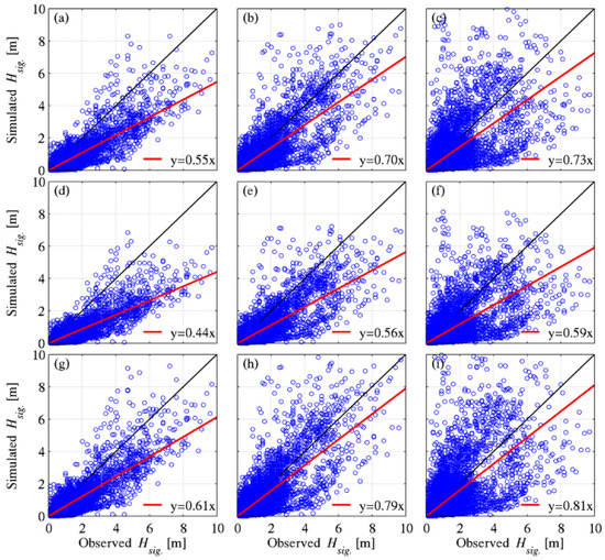
Figure 4.
Comparison of the simulated and observed significant wave heights based on the experimental conditions of the numerical model. (a) Case00 (+00 h); (b) Case00 (+06 h); (c) Case00 (+12 h); (d) Case01 (+00 h); (e) Case01 (+06 h); (f) Case01 (+12 h); (g) Case02 (+00 h); (h) Case02 (+06 h); (i) Case02 (+12 h).
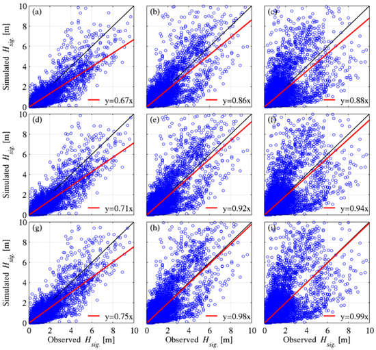
Figure 5.
Comparison of the simulated and observed significant wave heights based on experimental conditions of the numerical model. (a) Case03 (+00 h); (b) Case03 (+06 h); (c) Case03 (+12 h); (d) Case04 (+00 h); (e) Case04 (+06 h); (f) Case04 (+12 h); (g) Case05 (+00 h); (h) Case05 (+06 h); (i) Case05 (+12 h).
3.3. Comparison of Forecast Performance Based on the Changes in the Wind–Wave Interaction Growth Parameter
The bias and RMSE calculated using Equations (1) and (3) for each forecast lead time based on the numerical experimental results were used to analyze the effect of the change in on forecast performance. Figure 6a,b illustrate an analysis of the significant wave height, wave period, and wave direction. When was less than the initial setting value (= 1.65), the numerical model exhibited a tendency toward underestimation during the entire analysis period, and the forecast error increased. Conversely, when was greater than the initial setting value, the model tended to overestimate, and the forecast error decreased. However, when was set to a value greater than a fixed range, the forecast error increased with the increase in the forecast lead time. In the results of averaging the forecast error for each forecast lead time, the experimental conditions of Case06 indicated the smallest forecast error in the typhoon season. This is because when a strong wind field is generated, the actual phenomena interact and react more quickly than the model forecast. When was set based on the non-typhoon season, the wave development and propagation processes caused by the typhoon were not sufficiently reflected. Moreover, the sea wind forecast error and tendencies influenced the forecast performance of the wave model [44].
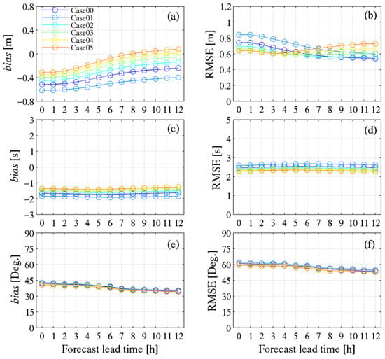
Figure 6.
(a) bias and (b) root mean square error (RMSE) of significant wave height; (c) bias and (d) RMSE of the wave period; (e) bias and (f) RMSE of the wave direction for each forecast lead time according to settings (Case00: = 1.65, Case01: = 1.15, Case02: = 2.05, Case03: = 2.45, Case04: = 2.85, Case05: = 3.25).
In addition to the analysis results regarding significant wave height, we analyzed the wave period and wave direction to understand the influence of the changes in the physical parameters, which indicate the wind forcing and wave interactions, on the physical components of the wave. Figure 6c,d depict the results of examining the wave period based on the values under different experimental conditions. As the forecast lead time increased, the model tended to underestimate under all experimental conditions. The forecast error exhibited a trend of increasing slightly at approximately 2.4 s for all forecast lead times despite the varying experimental conditions. Figure 6e,f illustrate the analysis results for the wave direction. We observed a positive bias under all experimental conditions at approximately 30–40° for each forecast lead time. Conversely, the forecast error was distributed at 50–60°, and it was difficult to discern a trend based on the values under different experimental conditions.
3.4. Forecast Performance of the Threshold Significant Wave Height
Figure 7, Figure 8 and Figure 9 illustrate the significant wave height () for each forecast lead time under different conditions and the observed significant wave height at the observation points of 22107, 22102, and 22105. In the non-typhoon season, no significant difference was observed between the forecast and observed results when the significant wave height was small. However, as the typhoon was northbound, the water surface displacement increased rapidly, and we observed relatively high wave heights even after the maximum significant wave height was attained. Above all, it seems to be significantly affected by the quality of the input wind field, and in general, the prediction error was relatively large at the beginning of the forecast lead time. In periods when the significant wave height increased and decreased rapidly, the peak wave heights were slightly different between the observation and model simulations. This can be attributed to the wave energy that was maintained larger than the forecast of the model. Moreover, a relatively large water surface displacement continued as the typhoon moved, and nonlinear effects that were more complex than those of the forecast of the wave model occurred due to the effects of the tracks of the typhoons, distance from the typhoon center, and wind intensity [46,47,48].
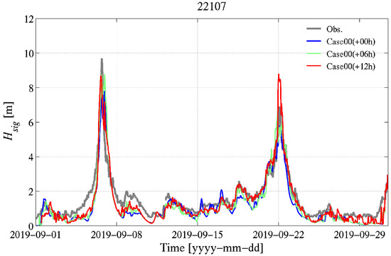
Figure 7.
Comparison of the observed and simulated significant wave heights for each forecast lead time at the observation point of 22107.
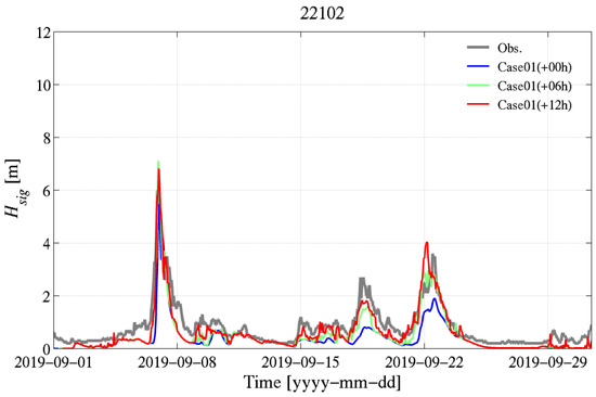
Figure 8.
Comparison of the observed and simulated significant wave heights for each forecast lead time at the observation point of 22102.
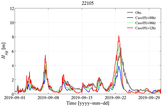
Figure 9.
Comparison of the observed and simulated significant wave heights for each forecast lead time at the observation point of 22105.
Table 3 summarizes the forecast performance for a threshold significant wave height averaged at all buoy observations corresponding to the numerical experiment conditions. The threshold wave height exists in the ranges of 0.0 m < ≤ 3.0 m, 3.0 m < ≤ 5.0 m, and 5.0 m < . We examined the significant wave height observation results and model forecast results based on the forecast lead time from 00 UTC on 1 September to 23 UTC on 30 September. We determined that = 3.25 in Case05 estimates the lowest forecast error in the entire experiment in the typhoon season. Furthermore, the effect of the growth parameter between wave and wind was identified as an important factor in determining the forecast error in the range of low significant wave heights, whereas the impact of the parameter was insufficient in the range of high significant wave heights.
Table 3.
Averaged root mean square error (RMSE) of the threshold significant wave height for each forecast lead time.
4. Conclusions
To construct a rapid refresh wave forecast model, we used KLAPS sea wind forecast data and examined the forecast performance of the wave model based on the changes in the physical parameter for the wind and wave interaction (). The wave model was executed by varying during the typhoon season, and the bias and RMSE for each forecast lead time were calculated to identify the numerical experimental condition that minimized the forecast error.
During the typhoon season, when increased beyond a fixed range, the model tended to overestimate the significant wave height, which simultaneously increased the forecast error with the increase in the forecast lead time. Additionally, when was less than the initial setting value of 1.65, the forecast error increased. Although a difference existed due to the experimental conditions, an error of approximately 0.6 m was generally observed. Furthermore, the model tended to underestimate the wave period, and a forecast error of approximately 2.4 s was observed. In the case of wave direction, the forecast error was distributed in the range of 50–60°; however, it was difficult to observe any trends based on the changes in . The that minimized the forecast error was identified by examining the significant wave height, and the obtained results were used in the rapid refresh wave model to analyze the forecast performance for the typhoon season. The forecast error was high during the initial forecast lead times, and the forecast error tended to decrease with the increase in the forecast lead time.
We concluded that the interaction between the waves and a strong wind field, such as a typhoon, was not sufficiently reflected due to the low that was used based on the results of a forecast performed during the non-typhoon season. Moreover, the inherent forecast error and tendencies of the atmospheric model influenced the forecast results of the wave model. The prediction results of the wave model are affected by the numerical scheme, the propagation and the integration time steps, wave–current interaction, and nonlinear interactions, and may cause differences from the observation results. However, in this paper, since numerical simulation experiments were conducted only in consideration of the effect of the input wind field, it is difficult to determine the effect on various factors in which the aforementioned prediction error occurs. Therefore, in subsequent studies, numerical simulations should be performed on the effects of the spectral and spatial resolutions and the effects of wave–current and wave–wave interactions on wave prediction. The prediction results of the wave model are verified using buoy observations and satellite data.
The results of this study can be used to effectively generate rapid refresh wave forecast data and marine weather status data that reflect rapidly changing marine weather conditions. Furthermore, the results of this study can aid in developing a rapid response technology for extreme weather conditions.
Author Contributions
Conceptualization, M.R. and K.K.; validation, M.R. and N.L.; formal analysis, M.R.; investigation, S.-M.O. and Y.O.; data curation, N.L. and S.-M.O.; writing—original draft preparation, M.R.; writing—review and editing, M.R. and H.-S.K.; visualization, M.R.; supervision, K.K. All authors have read and agreed to the published version of the manuscript.
Funding
This research was funded by the Korea Meteorological Administration Research and Development Program “Development of Marine Meteorology Monitoring and Next-generation Ocean Forecasting System, grant number KMA2018-00420”.
Institutional Review Board Statement
Not applicable.
Informed Consent Statement
Not applicable.
Data Availability Statement
The data and model output that support the findings of this study are available on request from the corresponding author.
Acknowledgments
We thank Il-Ju Moon of Jeju University for technical assistance and JongSook Park of Earthquake and Volcano Bureau of KMA for comments that significantly improved the manuscript.
Conflicts of Interest
The authors declare no conflict of interest.
References
- Ardhuin, F.; Magne, R. Current effects on scattering of surface gravity waves by bottom topography. J. Fluid Mech. 2007, 576, 235–264. [Google Scholar] [CrossRef]
- Ardhuin, F.; Tournadre, J.; Queffelou, P.; Girard-Ardhuin, F.; Collard, F. Observation and parameterization of small icebergs: Drifting breakwaters in the southern ocean. Ocean Modell. 2011, 39, 405–410. [Google Scholar] [CrossRef][Green Version]
- Ardhuin, F.; Roland, A.; Dumas, F.; Bennis, A.C.; Sentchev, A.; Forget, P.; Wolf, J.; Girard, F.; Osuna, P.; Benoit, M. Numerical wave modeling in conditions with strong currents: Dissipation, refraction and relative wind. J. Phys. Oceanogr. 2012, 42, 2101–2120. [Google Scholar] [CrossRef]
- Li, J.G. Propagation of ocean surface waves on a spherical multiple-cell grid. J. Comput. Phys. 2012, 231, 8262–8277. [Google Scholar] [CrossRef]
- Roland, A.; Zhang, Y.J.; Wang, H.V.; Meng, Y.; Teng, Y.C.; Maderich, V.; Brovchenko, I.; Dutour-Sikiric, M.; Zanke, U. A fully couple 3D wave-current interaction model on unstructured grids. J. Geophys. Res. Oceans 2012, 117, C00J33. [Google Scholar] [CrossRef]
- Toledo, Y.; Hsu, T.W.; Roland, A. Extended time-dependent mild-slope and wave-action equations for wave–bottom and wave–current interactions. Proc. R. Soc. Lond. A 2012, 468, 184–205. [Google Scholar] [CrossRef]
- Ardhuin, F.; Roland, A. The development of spectral wave models: Coastal and coupled aspects. In Proceedings of the 7th International Conference on Coastal Dynamics, Arcachon, France, 23–26 June 2013; Bonneton, P., Garlan, T., Eds.; University of Bordeaux: Bordeaux, France, 2013; pp. 25–38. [Google Scholar]
- Ponce de León, S.; Guedes Soares, C. Extreme Waves in the Agulhas Current Region Inferred from SAR Wave Spectra and the SWAN Model. J. Mar. Sci. Eng. 2021, 9, 153. [Google Scholar] [CrossRef]
- Tolman, H.L.; Chalikov, D. Source terms in a third-generation wind wave model. J. Phys. Oceanogr. 1996, 26, 2497–2518. [Google Scholar] [CrossRef]
- Ardhuin, F.; Herbers, T.H.C. Numerical and physical diffusion: Can wave prediction models resolve directional spread. J. Atmos. Ocean. Technol. 2005, 22, 886–895. [Google Scholar] [CrossRef]
- Tolman, H.L. User Manual and System Documentation of WAVEWATCH III Version 4.18. Technical Note; 2014. Available online: https://polar.ncep.noaa.gov/waves/wavewatch/manual.v4.18.pdf (accessed on 1 March 2014).
- Bouws, E.; Komen, G.J. On the balance between growth and dissipation in an extreme depth-limited wind-sea in the southern North Sea. J. Phys. Oceanogr. 1983, 13, 1653–1658. [Google Scholar] [CrossRef]
- Benoit, M.; Marcos, F.; Becq, F. Development of a third generation shallow-water wave model with unstructured spatial meshing. In Proceedings of the 25th International Conference on Coastal Engineering, Orlando, FL, USA, 2–6 September 1996; ASCE: Reston, VA, USA, 1996; pp. 465–478. [Google Scholar]
- Booij, N.; Ris, R.C.; Holthuijsen, L.H. A third-generation wave model for coastal regions: 1. model description and validation. J. Geophys. Res. Oceans 1999, 104, 7649–7666. [Google Scholar] [CrossRef]
- Tanaka, M. Verification of Hasselmann’s energy transfer among surface gravity waves by direct numerical simulations of primitive equations. J. Fluid Mech. 2001, 444, 199–221. [Google Scholar] [CrossRef]
- Babanin, A.V.; Makin, V.K. Effects of wind trend and gustiness on the sea drag: Lake George study. J. Geophys. Res. Oceans 2008, 113, C02015. [Google Scholar] [CrossRef]
- Rogers, W.E.; Babanin, A.V.; Wang, D.W. Observation-consistent input and whitecapping dissipation in a model for wind-generated surface waves: Description and simple calculations. J. Atmos. Ocean. Technol. 2012, 29, 1329–1346. [Google Scholar] [CrossRef]
- Rascle, N.; Ardhuin, F. A global wave parameter database for geophysical applications. Part 2: Model validation with improved source term parameterization. Ocean Modell. 2013, 70, 174–188. [Google Scholar] [CrossRef]
- Moghimi, S.; Van der Westhuysen, A.; Abdolali, A.; Myers, E.; Vinogradov, S.; Ma, Z.; Liu, F.; Mehra, A.; Kurkowski, N. Development of an ESMF based flexible coupling application of ADCIRC and WAVEWATCH III for high fidelity coastal inundation studies. J Mar. Sci. Eng. 2020, 8, 308. [Google Scholar] [CrossRef]
- Willebrand, J. Energy transport in a nonlinear and inhomogeneous random gravity wave field. J. Fluid Mech. 1975, 70, 113–126. [Google Scholar] [CrossRef]
- Hasselmann, S.; Hasselmann, K.; Allender, J.H.; Barnett, T.P. Computations and parameterizations of the nonlinear energy transfer in a gravity-wave spectrum. Part II: Parameterizations of the nonlinear energy transfer for application in wave models. J. Phys. Oceanogr. 1985, 15, 1378–1391. [Google Scholar] [CrossRef]
- Dommermuth, D.G.; Yue, D.K. A high-order spectral method for the study of nonlinear gravity waves. J. Fluid Mech. 1987, 184, 267–288. [Google Scholar] [CrossRef]
- Janssen, P.A.E.M. Quasi-linear theory of wind-wave generation applied to wave forecasting. J. Phys. Oceanogr. 1991, 21, 1631–1642. [Google Scholar] [CrossRef]
- Elfouhaily, T.; Thompson, D.; Vandemark, D.; Chapron, B. Weakly nonlinear theory and sea state bias estimations. J. Geophys. Res. Oceans 1999, 104, 7641–7647. [Google Scholar] [CrossRef]
- van Vledder, G.P. The WRT method for the computation of non-linear four-wave interactions in discrete spectral wave models. Coast. Eng. 2006, 53, 223–242. [Google Scholar] [CrossRef]
- Tayfun, A.; Fedele, F. Wave height distributions and nonlinear effects. Ocean Eng. 2007, 34, 1631–1649. [Google Scholar] [CrossRef]
- Donelan, M.A.; Babanin, A.V.; Young, I.R.; Banner, M.L. Wave-follower field measurements of the wind-input spectral function. Part II: Parameterization of the wind input. J. Phys. Oceanogr. 2006, 36, 1672–1689. [Google Scholar] [CrossRef]
- Rogers, W.E.; Kaihatu, J.M.; Hsu, L.; Jensen, R.E.; Dykes, J.D.; Holland, K.T. Forecasting and hindcasting waves with the SWAN model in the Southern California Bight. Coast. Eng. 2007, 54, 1–15. [Google Scholar] [CrossRef]
- Zieger, S.; Vinoth, J.; Young, I.R. Joint calibration of multiplatform altimeter measurements of wind speed and wave height over the past 20 years. J. Atmos. Ocean. Technol. 2009, 26, 2549–2564. [Google Scholar] [CrossRef]
- Liu, Q.; Babanin, A.V.; Guan, C.; Zieger, S.; Sun, J.; Jia, Y. Calibration and validation of HY-2 altimeter wave height. J. Atmos. Ocean. Technol. 2016, 33, 919–936. [Google Scholar] [CrossRef]
- Mao, M.; van der Westhuysen, A.J.; Xia, M.; Schwab, D.J.; Chawla, A. Modeling wind waves from deep to shallow waters in Lake Michigan using unstructured SWAN. J. Geophys. Res. Oceans 2016, 121, 3836–3865. [Google Scholar] [CrossRef]
- Montoya, R.D.; Osorio Arias, A.; Ortiz Royero, J.C.; Ocampo-Torres, F.J. A wave parameters and directional spectrum analysis for extreme winds. Ocean Eng. 2013, 67, 100–118. [Google Scholar] [CrossRef]
- Bingöl, C. Calibration and Evaluation of WAVEWATCH III under Extreme Conditions in Eastern Mediterranean and Aegean Sea Basin. Master’s Thesis, Middle East Technical University, Ankara, Turkey, August 2019. [Google Scholar]
- Abdolali, A.; Roland, A.; van der Westhuysen, A.; Meixner, J.; Chawla, A.; Hesser, T.J.; Smith, J.M.; Sikiric, M.D. Large-scale hurricane modeling using domain decomposition parallelization and implicit scheme implemented in WAVEWATCH III wave model. Coast. Eng. 2020, 157, 103656. [Google Scholar] [CrossRef]
- Abdolali, A.; van der Westhuysen, A.; Ma, Z.; Mehra, A.; Roland, A.; Moghimi, S. Evaluating the accuracy and uncertainty of atmospheric and wave model hindcasts during severe events using model ensembles. Ocean Dyn. 2021, 71, 217–235. [Google Scholar] [CrossRef]
- Kalourazi, M.Y.; Siadatmousavi, S.M.; Yeganeh-Bakhtiary, A.; Jose, F. WAVEWATCH-III source terms evaluation for optimizing hurricane wave modeling: A case study of Hurricane Ivan. Oceanologia 2021, 63, 194–213. [Google Scholar] [CrossRef]
- Ponce de León, S.; Bettencourt, J.H. Composite analysis of North Atlantic extra-tropical cyclone waves from satellite altimetry observations. Adv. Space Res. 2021, 68, 762–772. [Google Scholar] [CrossRef]
- Ardhuin, F.; Rogers, E.; Babanin, A.; Filipot, J.F.; Magne, R.; Roland, A.; van der Westhuysen, A.J.; Queffeulou, P.; Lefevre, J.M.; Aouf, L.; et al. Semiempirical dissipation source functions for ocean waves. Part I: Definition, calibration and validation. J. Phys. Oceanogr. 2010, 40, 1917–1941. [Google Scholar] [CrossRef]
- Alonso, R.; Santoro, P.; Solari, S. New wave hindcast for the Rio de la Plata Estuary. In Proceedings of the 36th International Conference on Coastal Engineering, Baltimore, MD, USA, 30 July–3 August 2018. [Google Scholar]
- Osinski, R.D.; Radtke, H. Ensemble hindcasting of wind and wave conditions with WRF and WAVEWATCH III® driven by ERA5. Ocean Sci. 2020, 16, 355–371. [Google Scholar] [CrossRef]
- Wu, J. Wind-stress coefficients over sea surface from breeze to hurricane. J. Geophys. Res. Oceans 1982, 87, 9704–9706. [Google Scholar] [CrossRef]
- Powell, M.D.; Vickery, P.J.; Reinhold, T.A. Reduced drag coefficient for high wind speeds in tropical cyclones. Nature 2003, 422, 279–283. [Google Scholar] [CrossRef]
- Huang, Y.; Weisberg, R.H.; Zheng, L.; Zijlema, M. Gulf of Mexico hurricane wave simulations using SWAN: Bulk formula-based drag coefficient sensitivity for Hurricane Ike. J. Geophys. Res. Oceans 2013, 118, 3916–3938. [Google Scholar] [CrossRef]
- Roh, M.; La, N.R.; Oh, S.M.; Kang, K.R.; Chang, P.H. Development and verification of a rapid refresh wave forecasting system. J. Korean Soc. Coast. Ocean Eng. 2020, 32, 340–350. (In Korean) [Google Scholar] [CrossRef]
- WMO Guide to wave analysis and forecasting. In WMO-No. 702, 2nd ed.; World Meteorological Organization (WMO): Geneva, Switzerland, 1998; p. 73.
- Large, W.G.; Pond, S. Open ocean momentum flux measurements in moderate to strong winds. J. Phys. Oceanogr. 1981, 11, 324–336. [Google Scholar] [CrossRef]
- Moon, I.J.; Ginis, I.; Hara, T.; Tolman, H.L.; Wright, C.W.; Walsh, E.J. Numerical simulation of sea surface directional wave spectra under hurricane wind forcing. J. Phys. Oceanogr. 2003, 33, 1680–1706. [Google Scholar] [CrossRef]
- Cardone, V.J.; Cox, A.T. Tropical cyclone wind field forcing for surge models: Critical issues and sensitivities. Nat. Hazards 2009, 51, 29–47. [Google Scholar] [CrossRef]


Publisher’s Note: MDPI stays neutral with regard to jurisdictional claims in published maps and institutional affiliations. |
© 2021 by the authors. Licensee MDPI, Basel, Switzerland. This article is an open access article distributed under the terms and conditions of the Creative Commons Attribution (CC BY) license (https://creativecommons.org/licenses/by/4.0/).