Abstract
Electronic charts and marine radars are indispensable equipment in ship navigation systems, and the fusion display of these two parts ensures that the vessel can display dangerous moving targets and various obstacles on the sea. To reduce the noise interference caused by external factors and hardware, a novel radar image denoising algorithm using the concept of Generative Adversarial Network (GAN) using Wasserstein distance is proposed. GAN focuses on transferring the image noise distribution between strong and weak noise, while the perceptual loss approach is to suppress the noise by comparing the perceptual characteristics of the output after denoising. Afterwards, an image registration method based on image transformation is proposed to eliminate the imaging difference between the radar image and chart image, in which the visual attribute transfer approach is used to transform images. Finally, the sparse theory is used to process the high frequency and low frequency subband coefficients of the detection image obtained by the fast Fourier transform in parallel to realizing the image fusion. The results show that the fused contour has a high consistency, fast training speed and short registration time.
1. Introduction
With the development of science and technology, great progress has been made in ship collision avoidance technology. However, the rapid growth in the number of ships has made managing maritime traffic extremely complex. Although many ships are equipped with collision avoidance, accidents, such as ship collision and ships hitting rocks, occur from time to time. Such accidents not only cause significant property losses, but also cause serious damage to the marine environment and even casualties [1]. The causes of accidents are mainly due to the ship navigation information, which mainly comes from navigation radar images and electronic charts, obtained by the ship officer not being timely or accurate.
Marine radar, one of the most important navigation technologies, can perceive the surrounding target information in extreme environments, and analyze it in order to realize the function of target recognition and navigation. The Electronic Chart Display Information System (ECDIS) is a platform used for displaying chart information based on computer technology, which can provide accurate water environment data for the ship’s crew. Both devices have certain limitations. Ship marine radars can only provide target echo information, while a single ECDIS displays an information-related chart. However, the fusion of these two images in this research will not only help ships’ crews to better understand the environment of the sea area, but to also improve the safety of ship navigation.
As the image information provided by ship marine radar has certain noise that affects normal observation of the radar image, it is necessary to preprocess the noise. For a raw image with noise, the processing affected by using convolutional neural network (CNN) [2] is superior to the traditional wavelet transform method. The GAN [3] model endows people with a mode of thinking by using the generative model and the discriminant model, in which the generative model is applied for training and learning, and the discriminant model is utilized to judge whether the generation model is close to the truth until the discrimination model can no longer judge the “authenticity” of the generation model. Therefore, a GAN model based on Wasserstein distance is proposed to preprocess the image denoising.
Edge detection is regarded as an important steps in image fusion, and is mainly carried out using the Roberts operator, Sobel operator, or Canny operator, etc., [4]. Canny edge detection [5,6] can achieve a better solution when compared with other edge detection algorithms, and thus it has become one of the standards used to evaluate edge detection methods. In most cases, the low threshold QE and high threshold QS are set by using Canny edge detection to realize edge detection based on a multi-stage algorithm. In traditional methods, these two thresholds need to be manually intervened, and it is usually difficult to select the appropriate threshold for different images. An improved method [7] is proposed to set the threshold based on the gray histogram theory, however, this can produce certain false edges, resulting in inaccurate detection results. To obtain Qe, the Otsu algorithm [8] is proposed and the results show that it is a new valuable edge extraction method. It should be noted that the two thresholds above are defined as global values. However, this approach is limited to the local features for images with a complicated background. This research presents a local adaptive Canny edge detection method, which can better highlight the features of the image, has fast processing speed and is easy to implement.
For image registration, image feature point extraction and matching are the key step. Scale Invariant Feature Transform (SIFT) is one of the basic algorithms, and has been widely utilized in the image registration field [9,10] due to its invariance of scale and rotation. However, the SIFT algorithm still has some shortcomings [11]. The SIFT algorithm improves the speed by introducing Hessian matrix and calculating the integral image, but it is weak in terms of extracting feature points with smooth edges. Meanwhile, the SIFT algorithm based on Harris point ensures the Harris corners scale invariant by constructing scale space, and uses the idea of Forsnter’s operator to accurately locate the corners. The purpose of image registration is to acquire the transformed matrices between radar echo image and electronic chart image. In this research, the image registration approach adopted mainly contains the following two aspects. On the one hand, a visual attribute conversion approach is designed and utilized in image conversion to avoid the imaging differences due to its depth image analogy. On the other hand, the generated radar echo image is matched with the original radar echo image, and the corresponding image is then mapped to the electronic chart to obtain the final matching result. Finally, the final corresponding relationship can be obtained by using the SIFT operator.
In general, the level of image fusion can be classified into three types: pixel level, feature level, and decision level. According to the feature boundary given by the chart and radar image, the idea of feature-level fusion is used for image fusion. In [12], ECDIS is covered by marine radar echo to verify the applicability of navigation safety. The real-time overlap of ECDIS and radar echo images are comprehensively evaluated in [13,14]. In [15], an image fusion technique from radar echo image and electronic chart image based on a neural network is applied to distinguish image characteristics. The above approaches utilize diverse operators to identify the characteristics of radar echo and deformation of the target.
The main contributions of the proposed work are as follows. Firstly, the method of combining Wasserstein distance and perceptual loss is used to denoise the radar echo image and obtain a high-quality radar image. Secondly, the local adaptive Canny operator is applied to identify the edge feature of the radar echo, and the multimodal image registration method is used to implement the image registration between the radar echo image and electronic chart. Finally, the effective perceptual fusion of the ship marine radar image and electronic chart are realized by using the combination of sparse theory and fast Fourier transform (FFT), and the quality of the fused image is evaluated by using the different algorithm.
2. Image Denoising Algorithm Based on WGAN
In this research, a GAN with the Wasserstein framework based on Wasserstein distance, namely WGAN, is presented to address the problem of image blur and non-uniform deviation [16]. The Wasserstein distance is utilized as the evaluation parameter between distribution and perceptual loss, and the difference between images in the feature space established by perceptual loss calculation is used. Suppose is the radar image with noise, and is the corresponding normal radar echo. The major purpose of the noise reduction approach is to find a function G that can map z to q. To compare the data distribution of GAN, WGAN using Wasserstein distance can replace Jensen-Shannon (JS) divergence. Therefore, the problem is transformed into one of solving the maximum and minimum values to solve the discriminator D and generator G [17].
where E( ) represents the expectation operator, q* means the uniform sampling along the straight line between the generated sample and the actual sample, and k is a constant weight. The Wasserstein distance is estimated by using Eq[D(q)] and Ez[D(G(z))], while the gradient penalty term is determined by using kEq*[(||∇q*D(q*)||2−1)2].
Although the WGAN network generator converts high noise data distribution to low noise data distribution, a loss function is added into the network to preserve the image data and information. Usually, the mean square error loss function is used to minimize the pixel-level error between the denoising patch G(z) and image patch [18]. However, the mean square error loss function may generate blurred images and then lead to image distortion. Hence, this research uses the perceptual loss function defined in the feature space to replace the variance loss function.
where is the feature extractor, where the pre-trained VGG-19 network is used as the feature extractor. In feature space, w*, d* and h* represent the width, depth and height, respectively, and represents the Frobenius norm. The VGG-19 network is composed of 16 convolution layers and 3 full connection layers. The output of the 16th convolutional layer senses the loss function, in which the loss function WVGG(G) can be defined as:
After Equations (1) and (3) are resolved, the combined joint loss function LWGAN(D,G) is:
where μ* means a weight value, which is mainly used to adjust the relation between the WVGG(G) and LWGAN(D,G).
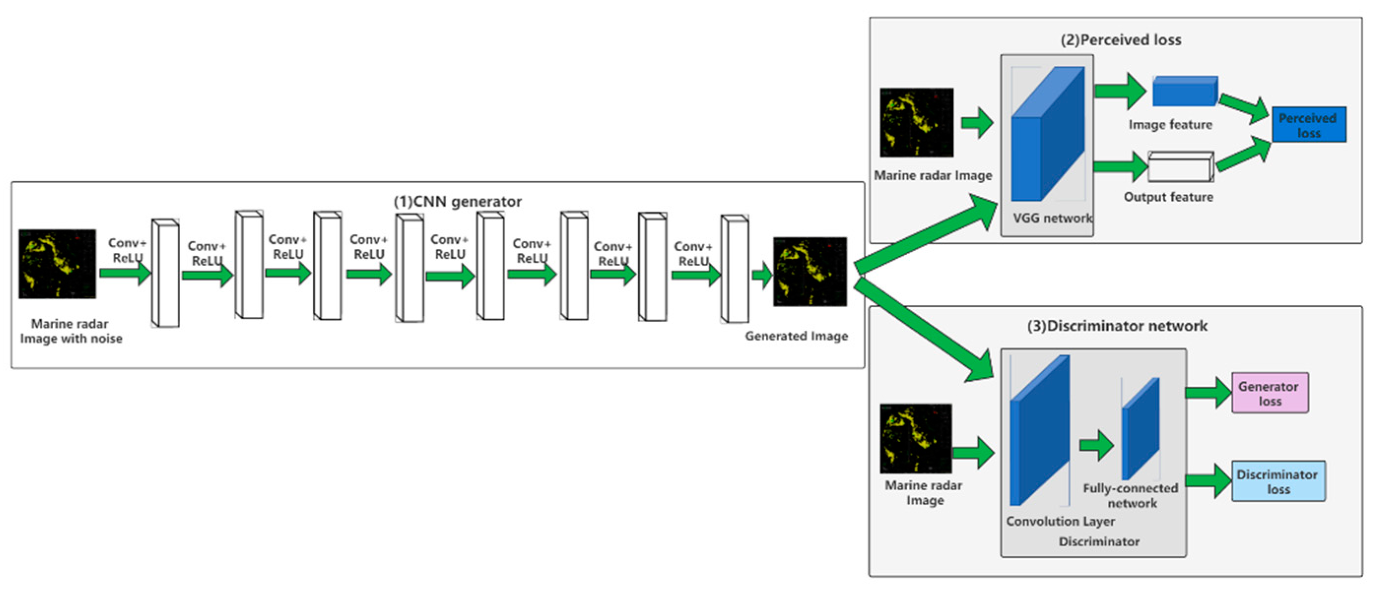
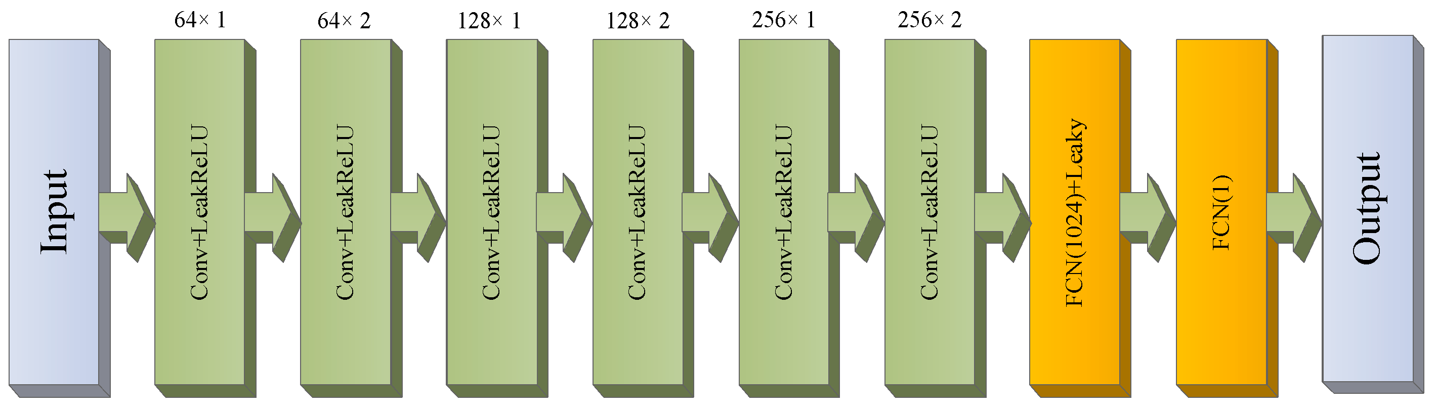
The WGAN-VGG framework is shown in Figure 1, where the generator G contains eight convolutional layers of CNN. Each convolution layer uses a 3 × 3 kernel. Due to this stacked structure, this network can cover enough large receptive fields. There exist 32 filters among the first seven hidden layers of G, and the last layer only generates a feature map of a 3 × 3 filter, namely, the output of G. Rectifying Linear Unit (ReLU) is used as the activation function. For feature extraction, the input of the pre-trained VGG network contains the normal image and the denoising output image G(z), meanwhile, the target loss can be calculated according to the features extracted from the designated layer of Formula (4). WGAN limits the gradient of discrimination network D by adding an additional loss. After sufficient training, the gradient of the discrimination network is stable near 1, and the gradient is stabilized by adding gradient penalty term. To maintain the VGG parameters unchanged, the weight of G is updated by using the reconstruction error backpropagation. As shown in Figure 2, the discriminator network D are composed of six convolution layers, in which the first two convolution layers have 64 filters, the middle two convolution layers have 128 filters, and the last two convolution layers have 256 filters. The image patches are used to train the network, and are then extended to the whole image. The activation function used in the discrimination network is the Rectifying Linear Unit (ReLU) function, which contains six filter cores, with the number of cores ranging from 64 to 256. After passing through the sigmoid activation layer, the final 256 feature map is closer to the navigation radar image [17].

Figure 1.
The structure of WGAN-VGG network.
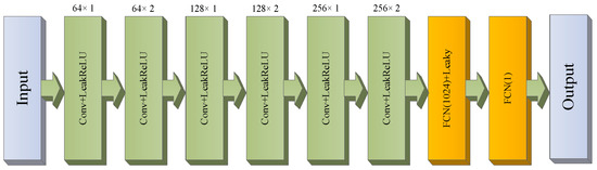
Figure 2.
The structure of the discriminator network.
3. Image Registration
3.1. Local Adaptive Canny Edge Detection
For the sake of enhancing the recognition precision of target edge detection, a local adaptive recognition method using a local high threshold Qs and low threshold Qe is proposed. The image is divided into eight subregions, and each subregion calculates a different Qs and Qe. Compared with global Canny edge detection, local adaptive Canny edge detection can lead to some edge discontinuity, but this method can detect more edges and produce more detailed results for subsequent processing.
When the Canny operator is used for edge detection, the edge information can be decided by the size of the thresholds [19]. Therefore, the high threshold is inversely proportional to the retained edge information, and is also inversely proportional to inaccurate edge. For the sake of achieve richer edge information, we take the average gradient amplitude s* and the standard deviation l* as the parameters of high threshold Qs, which can be defined as:
where c* means the adjustable coefficient, principally to avoid the loss of some edge details caused by the direct addition of s* and l*. In [20], experiments show that when the condition of 0.5 < c* < 0.7 is satisfied, the effect of edge detection tends to be more ideal, therefore c* is 0.6 in this research. The standard deviation of average gradient amplitude s* and pixel gradient amplitude l* is defined as:
where Kx × Ky denotes the total pixels, while GM(a*,b*) denotes the gradient of pixels.
The procedures are summarized below:
- Choose the number of marine radar echo images to use, and then segment the entire image as needed.
- The local high threshold Qs and low threshold Qe of each marine radar echo image are calculated respectively according to the experiment in this research, Qe is 0.4 Qs.
- A Gaussian filter is used to filter Gaussian noise, and the size and direction of the gradient are calculated [21].
- Non-maximum suppression is utilized to gradient values. Get rid of part of the non-edge pixels and retrieval candidate edges to highlight the most possible edge pixels.
- The Qs and Qe are used to identify and link the edge of each radar echo image. When the gradient of a pixel is greater than Qs, the pixel is marked as an edge pixel, but when the gradient of a pixel is lower than Qe, the pixel is defined as the background. The processed marine radar echo image is merged into a complete image.
3.2. Image Conversion
3.2.1. Mapping Relationship
Firstly, the radar echo image of edge detection is used as the input, and the pyramid features are constructed by using the pre-trained CNN. Before reconstruction, it is necessary to establish the position mapping between the feature maps, and then use the bidirectional nearest neighbor field search to set up the mapping relationship. The definition of energy equation can be expressed as [22]:
where P and Q denote the patches, and their corresponding centers are located in the mapping point. L is the scale. F(x) means the vector of x, and its normalization feature means .
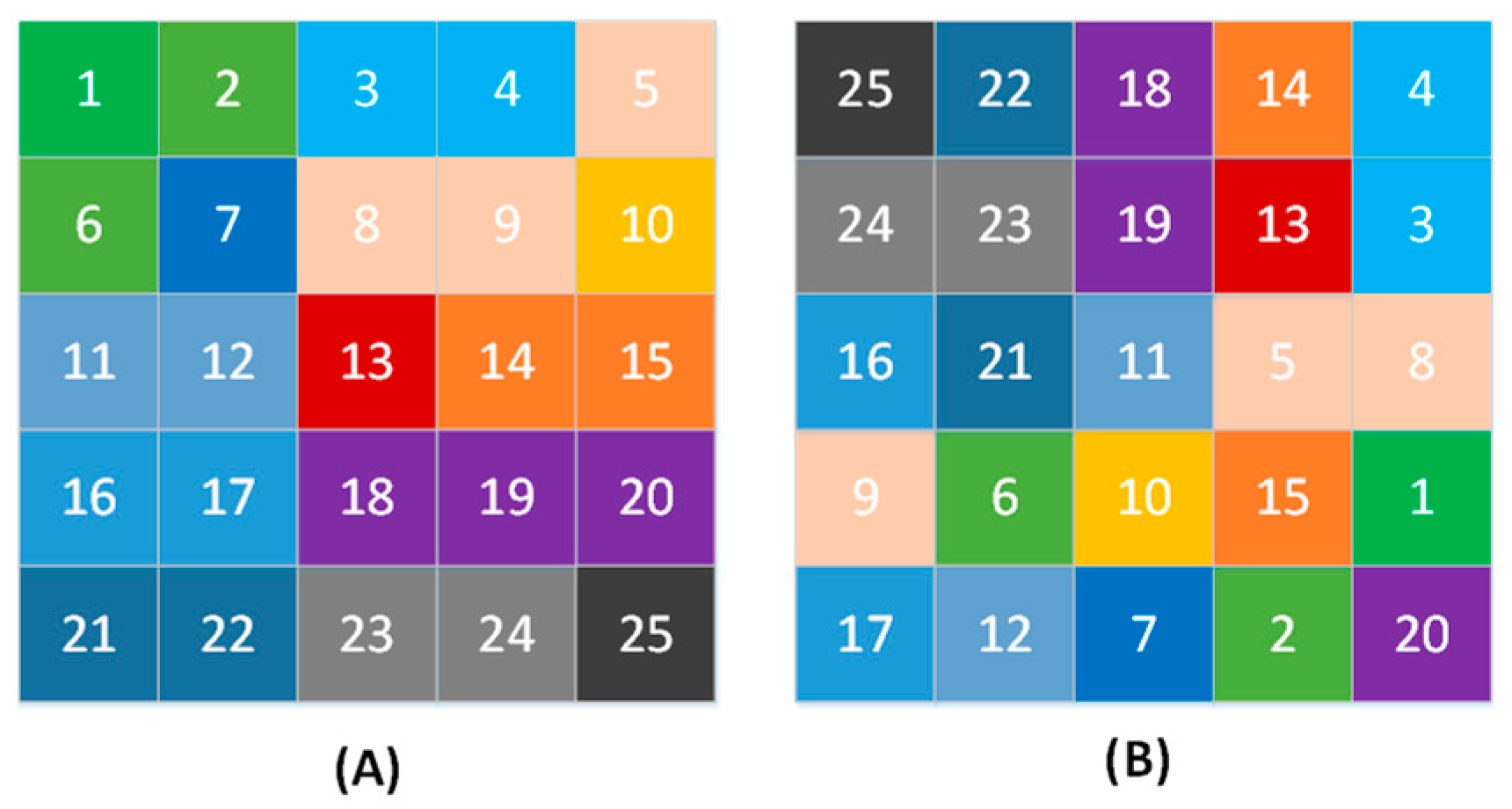
The energy function is optimized by using the nearest neighbor field search method to obtain the relationship of feature mapping. The analogous image can be achieved by reconfiguring each pixel in Figure 3B.

Figure 3.
(A) Feature map for image A. (B) Feature map for image B.
3.2.2. Restructure
To restore the low-level relational feature mapping on the basis of the high-level feature mapping, the scales between the levels are different. Before the reconstruction of the layer, it is necessary to ensure that the size of the feature mapping is the same. Hence, the upper features can be reconstructed by using the gradient-based optimization approach [23]. Firstly, the corresponding position relationship between features is determined. The second step is to remove part of the network that constructs the functional relationship between the P−1 layer and the P layer, with the goal of minimizing the loss function to obtain better and . The loss function is defined as:
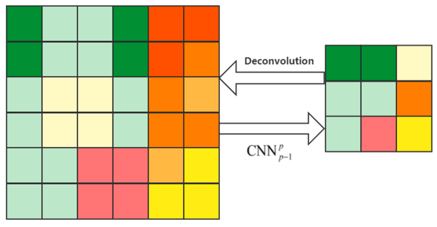
where represents the deconvolution result of , as shown in Figure 4, represents the function from P−1 to P layers. The superscript result can be obtained by minimizing . The calculation method of is as follows:
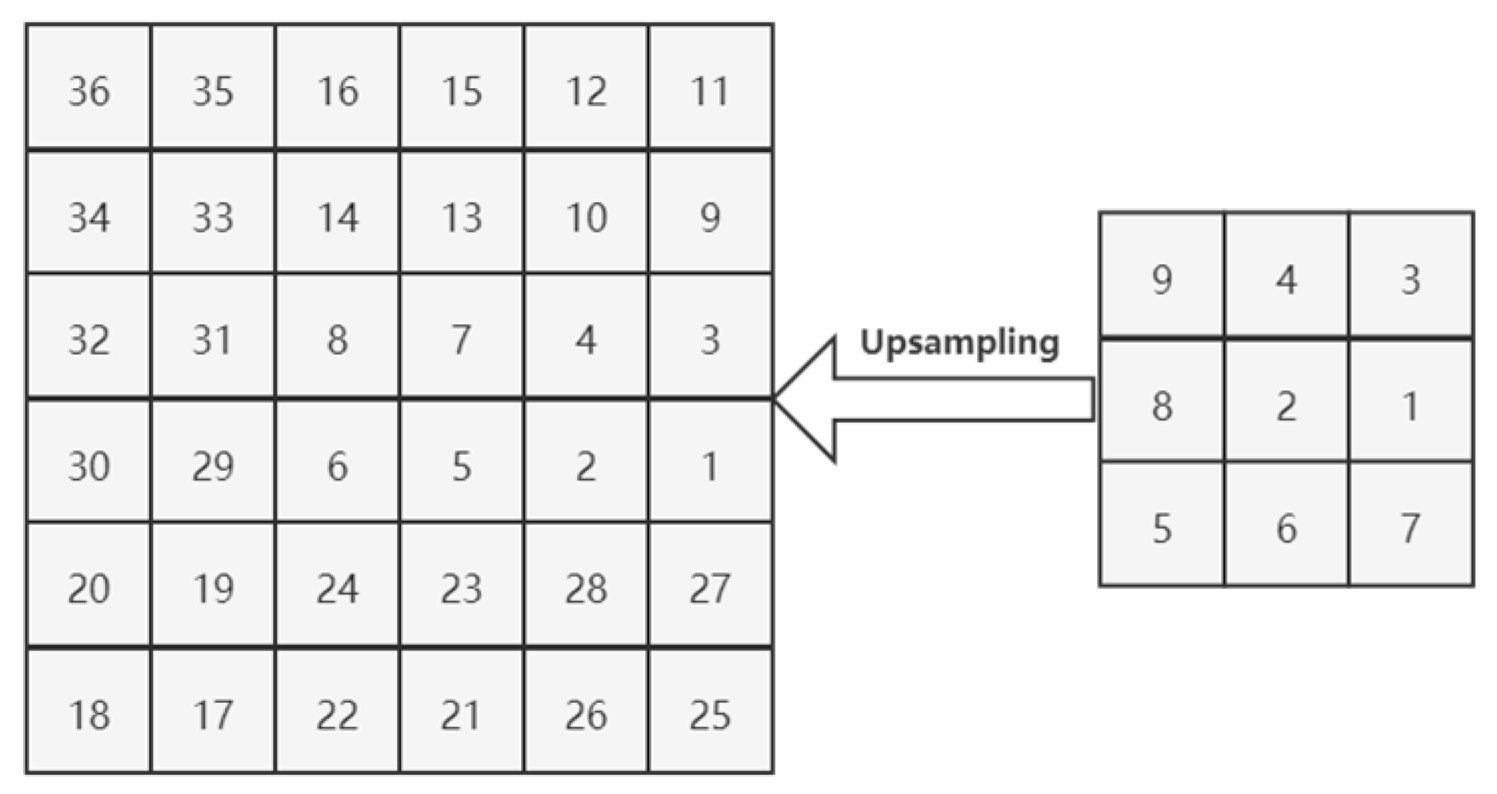
where is the weight mapping of the response at the P−1 level, and is the product of elements. After the feature mapping is restored to the shallow layer, it is necessary to unify the mapping scale, and directly sample and , as shown in Figure 5, which is regarded as the initialization of the shallow mapping relationship.

Figure 4.
Deconvolving.

Figure 5.
Upsampling.
3.3. Image Matching
In the process of image conversion, the pixel-level mapping relationship between radar echo image and electronic chart can be acquired. We only use this relationship in image conversion to solve the problem of difference between images, and the classical local feature operator is used to align image.
We use SIFT to obtain the final correspondence, mainly because SIFT has certain advantages in the registration assignment. Moreover, SIFT utilizes the sub-pixel interpolation method to search the key points accurately. Therefore, the precision of the algorithm is significantly improved. After matching the radar image and electrical chart image, the corresponding relationship is mapped back to the initial image to obtain the final matching image.
4. Fusion Algorithm
4.1. Sparse Theory
Sparse theory [24] is an important step in image fusion. It represents as much knowledge as possible with few resources. This representation also brings one significant advantage: fast computing speed. Sparse representation mainly gathers the obvious structural information in the image field into fewer atomic images in the dictionary, and the integration of atomic images can form an over complete dictionary. Due to the redundancy of the dictionary, the signal can be represented by the linear integration of a small number of atoms in the dictionary. The representation with the least number of atoms in the representation is sparse representation. Its essence is to seek the minimum atoms from the base or dictionary, and use these minimum atoms and sparse coefficient linear combination to represent information, namely, the radar echo image. As such, the least sample representation is sparse representation: suppose there are r classes, each class of a single sample is represented by column vector evj in matrix E. Class v contains z samples, the expression is as follows:
o can be expressed by the combination of samples of class v, the expression is as follows:
where 0 < < 1 is the linear combination coefficient with random value.
4.2. Fast Fourier Transform
Fast Fourier Transform [25] (FFT) is the collective name of the fast and efficient calculation approach for calculating Discrete Fourier Transform (DFT), and as such, this method can significantly decrease the calculation amount of DFT. In particular, the more times that the N sampling points are transformed, the more crucial the sparing of FFT algorithm is. FFT algorithm inherits the characteristics of parity, virtuality and realness of the discrete Fourier transform, and improves the dependence of discrete Fourier transform in terms of image and intensity transform. The radar echo image after FFT transform has low frequency in the center position and high frequency scattering around.
4.3. Dictionary Learning
Dictionary learning [26] is also called sparse coding. The original sample is represented by matrix Y*, the dictionary matrix is represented by D*, and the entries in the dictionary, i.e., atoms, are represented by column vector dk. The method to find the dictionary is sparse matrix, which is represented by X*. The process of finding the dictionary is that the matrix multiplication is represented by DX*, and the main idea of dictionary learning is to use the dictionary matrix containing K atoms dk. The sparse linear table is the original sample; that is, there is a sparse matrix. The above problems can be described as the following optimization problems in mathematical language:
where X* is the sparse coded matrix, xi* (i = 1,2,…, k) is the row vector, represents the zero order norm and the number of non-zero numbers in the vector. This is done in order to make it as sparse as possible and make non-zero elements as few as possible.
The objective function means to minimize the error between the dictionary and the original sample, that is, to restore the original sample as much as possible. The limiting condition is , which means that the way of looking up the dictionary should be as simple as possible; that is, X* should be as sparse as possible. The objective function is an optimization problem and constraints, which can be transformed into an unconstrained optimization problem by using the Lagrange multiplier method:
There are two optimization variables, D and X*, in the formula. For the sake of solving this optimization issue, one optimization variable is generally fixed and the other variable is optimized alternately. The sparse matrix X* in the above formula can be solved by using existing classical algorithms, such as Minimum Absolute Contraction (MAC), Selection Operator (SO) and Orthogonal Matching Pursuit (OMP).
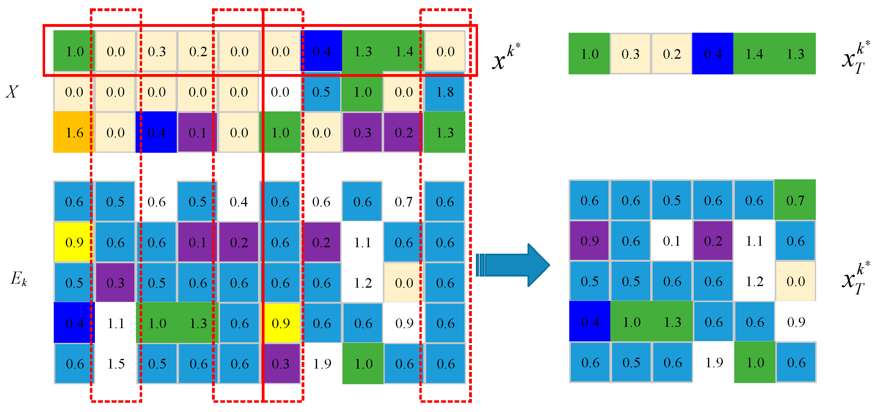
Assuming that X* is known, the dictionary column will be updated by column. Next, only the k-th column of the dictionary will be updated. Record dk as the k-th column vector of dictionary d* and Xk as the k-th row vectors of sparse matrix X*:
The residual in the above formula is:
At this time, the optimization problem can be described as:
Therefore, we need to discuss the optimal parameters dk and Xk. This is a least square problem. We can use the SVD method to solve two optimization variables. However, it should be noted that Ek cannot be directly used to solve, otherwise the new Xk is not sparse. Therefore, it is necessary to extract the position where the corresponding Xk in Ek is not zero to obtain a new Ek. The flow chart and detailed parameters is shown in Figure 6:
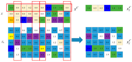
Figure 6.
Dictionary update map.
Suppose we want to update the atom in column 0, we find the position of zero in Xk, and then delete the position corresponding to Ek to get . At this time, the optimization issue can be depicted as follows:
Therefore, it is necessary to find the optimal:
Take the first column vector of the left singular matrix U as dk = u1, that is dk, and the product of the first row vector and the first singular value of the right singular matrix as , that is . After obtaining , update it to the original accordingly.
4.4. Fusion Algorithm
Firstly, the radar echo image is decomposed into high-frequency subband and low-frequency subband by FFT. The high-frequency subband involves important data of the radar echo image, and the low-frequency subband involves the approximate image of the radar echo image. The high-frequency subband coefficients are fused by using the high-frequency fusion rule, while the low-frequency subband coefficients are trained to obtain the dictionary. Finally, the fused image of electronic chart and radar echo image is obtained by inverse FFT. The fusion strategy is as follows.
- Taking the region coefficient of radar echo image R, the approximate coefficient after image fusion is denoted as .
- Solve the relative standard deviation of and , denoted as and .
- Calculate the absolute value of the difference between and , denoted as .
- Solve the energy value of .
- Judge the three values of , and , select the most representative parameters, denoted as .
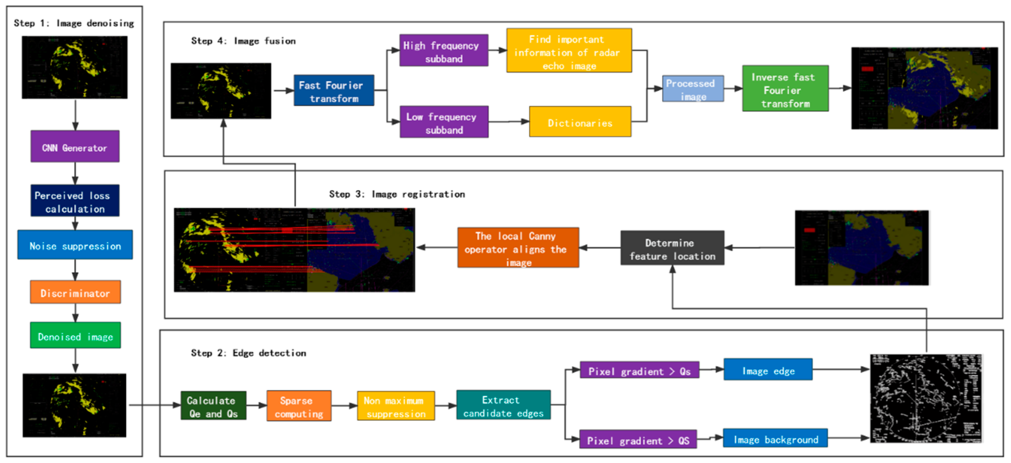
The overall architecture of perceptual fusion of electronic chart and navigation radar image is shown in Figure 7.

Figure 7.
Overall architecture diagram of perceptual fusion.
5. Experimental Results and Analysis
5.1. Image Denoising and Edge Detection
The data set of radar image is the radar image provided by “Yukun” sailing in the sea area of Dalian port, China in 2020. In our experiment, we randomly extracted 10,096 pairs of image patches from 1000 radar images as our training input and label. The patch size is 64 × 64. In addition, we extracted 5056 pairs of image patches from another 500 images for verification. When implementing image denoising, the Adam algorithm is used to optimize the network. The minimum batch is 128, which is selected according to our experimental experience μ* = 0.1.
In order to verify the convergence of WGAN, of Equation (1) is plotted as the estimated Wasserstein value. As can be seen in Figure 8, although the attenuation rate becomes smaller, the increasing number of epochs does reduce the W-distance. For WGAN-VGG, the introduction of VGG loss helps to enhance perception, but at the cost of damage to the loss measurement.
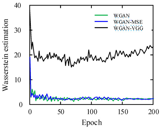
Figure 8.
Verification curve of WGAN convergence.
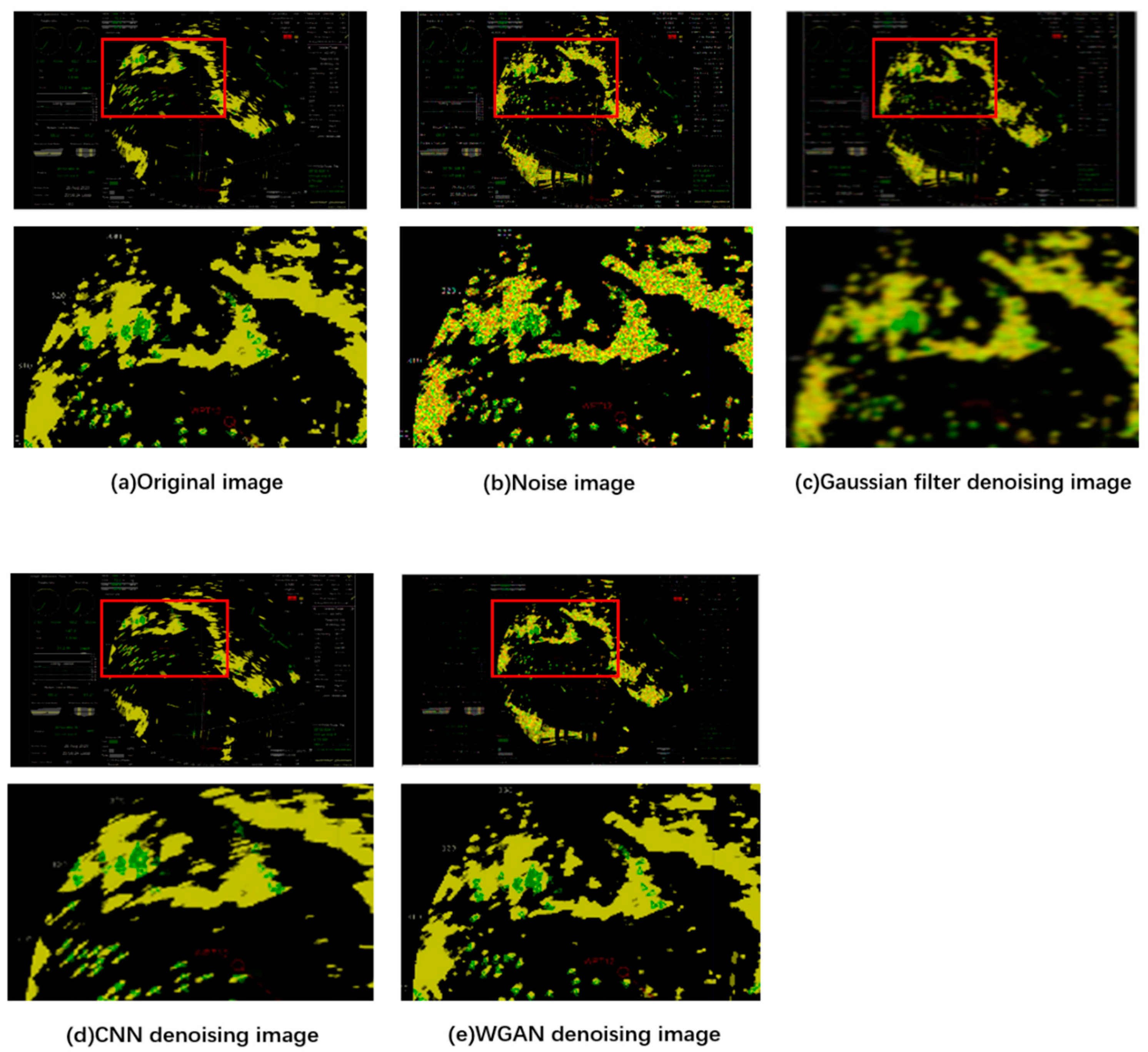
The radar echo image is based on the Gaussian filter [27], CNN [28] and WGAN [29] methods for image denoising. The contrast images are shown in Figure 9.
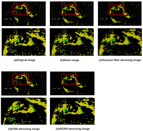
Figure 9.
Image denoising contrast diagram.
It can be seen from the comparison figure that all methods show a certain denoising ability. The Gaussian filter method blurs the image and generates other interference. Compared with the Gaussian filter, CNN can reduce the effect of noise by averting excessive smoothing, but compared with WGAN, noise can still be observed. This is mainly because the WGAN network uses a post-processing approach. The lost information in the reconstruction process is hard to recover, which is a limitation of all post-processing approaches. Sometimes it will over-smooth some fine structures. However, the WGAN image is visually similar to the radar echo image. By using the VGG loss, the human perception knowledge embedded in the VGG network is transferred to the radar echo image to achieve the most positive noise reduction effect. Table 1 shows the peak signal noise ratio (PSNR) and structural similarity index (SSI) of each image denoising effect map as the objective criteria for evaluating the performance of the algorithm. It can be seen from the table that the PSNR and SSI values of WGAN method are higher than those of the Gaussian filter method and CNN method. Compared with other methods, WGAN achieves the better denoising effect.

Table 1.
Evaluation table of edge detection algorithm.
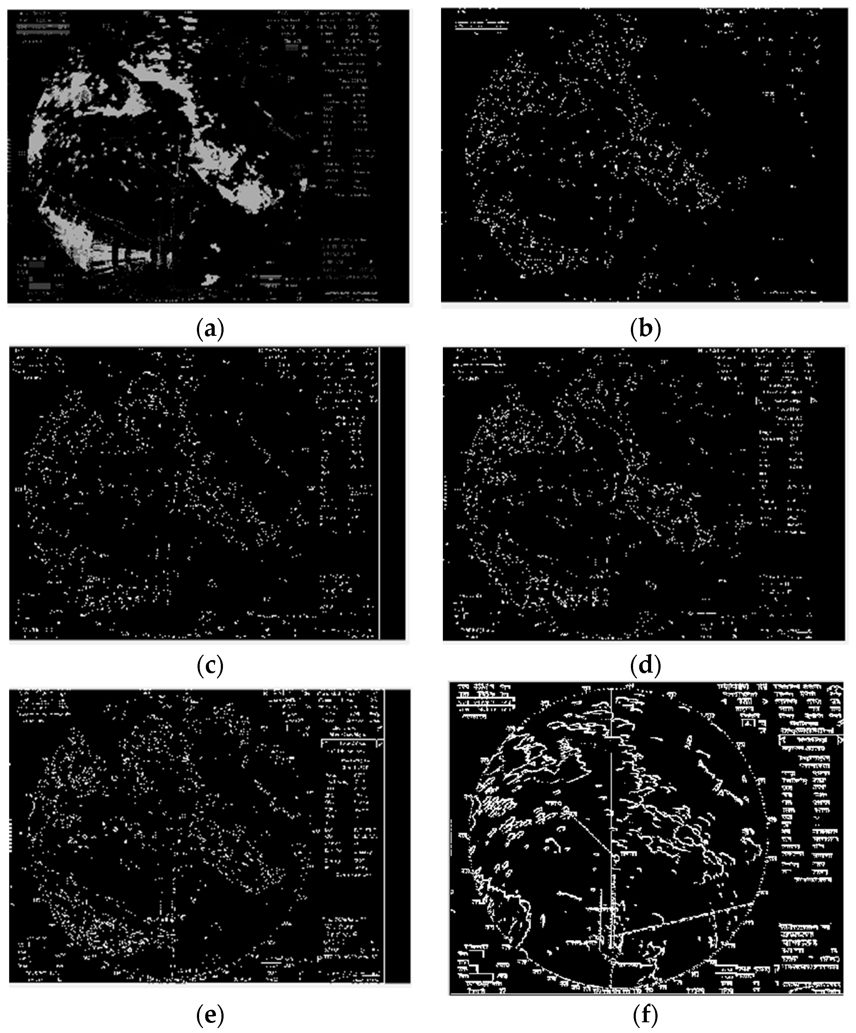
For the sake of verifying the availability and dependability of the proposed image edge detection method, taking the radar echo image as an example, the existing classical Sobel operator detector, Roberts operator detector, Prewitt operator detector and the improved Canny operator detector are compared. The experimental environment is intel i5-65003.20-0ghz processor and 8 GB memory. The simulation software is Matlab 2018a. All marine radar images have a width of 1920 pixels, a height of 1080 pixels and a total number of 1920 × 1080, with the horizontal and vertical resolutions being 96 dpi. The effect of the algorithm in edge continuity and positioning accuracy is verified. According to the experiment, the edge detection effect is better when c* is 0.6. As shown in Figure 10, when the traditional Canny operator of Gaussian function is used for image smoothing, the high-frequency edge is smoothed out, and in some cases even the edge is lost. The Roberts operator, which can detect rich edge details, contains much useless information. For the Sobel operator, no good recognition results are obtained because some details of the marine radar echo are ignored. The LoG operator decreases some interference from non-edge points to a certain extent, but there are still a small number of incorrect edges, resulting in edge discontinuity and discontinuity. The LoG operator has a strong anti-interference ability, but some edges cannot be detected. In addition, the proposed local adaptive Canny edge presents better edge detection influence among the various operators.
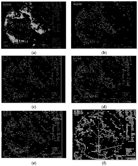
Figure 10.
The edge detector detects the image. (a) Original radar image, (b) Traditional Canny edge detection diagram, (c) Roberts operator for image detection, (d) Roberts operator for image detection, (e) Log operator for image detection, (f) Improved Canny operator for image detection.
The PSNR, SSI and the running time of the algorithm are counted respectively as the objective criteria to evaluate the performance of the two algorithms. The results are shown in Table 2. By comparing the data in the table, it can be seen that the improved Canny operator is better than other edge detection algorithms in terms of PSNR, SSI and running time, and can detect edges more accurately and filter out false edges.
Table 2.
Evaluation table of edge detection algorithm.
5.2. Image Registration
In order to verify the effectiveness of this method, the resolution of navigation radar image and electronic chart is 1920 × 1080. The RANSAC (random sample consensus) algorithm is used, and the ratio is set to 0.85. A higher value of PSNR indicates the better quality of image matching. According to the experiment, when the threshold value is 0.8 and the step size is 0.06, the value of PSNR is higher. We select the SIFT registration method and SURF registration method for comparison. The SIFT denoising effect and SURF denoising effect are shown in Figure 11 and Figure 12, respectively.

Figure 11.
SIFT registration rendering image.
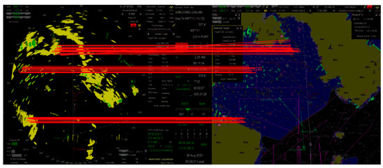
Figure 12.
SURT registration rendering image.
Table 3 lists the evaluation performance by using the Root Mean Square Error (RMSE), Correct Corresponding Number (CCN) and Peak Signal Noise Ratio (PSNR). The results of image registration and comparison show that the pixel-level mapping relation between the radar echo image and electronic chart can be acquired by these two algorithms. But through the SIFT denoising method, the root mean square error is small, the number of correct correspondences of feature points is more, and the image registration effect is better. The average time of a single test image is 0.15 s, the registration is completed in 0.5 s, and the image registration rate is about 95%, which shows that the algorithm can operate in real-time and has accuracy.
Table 3.
Image registration comparison results.
5.3. Image Fusion Effect
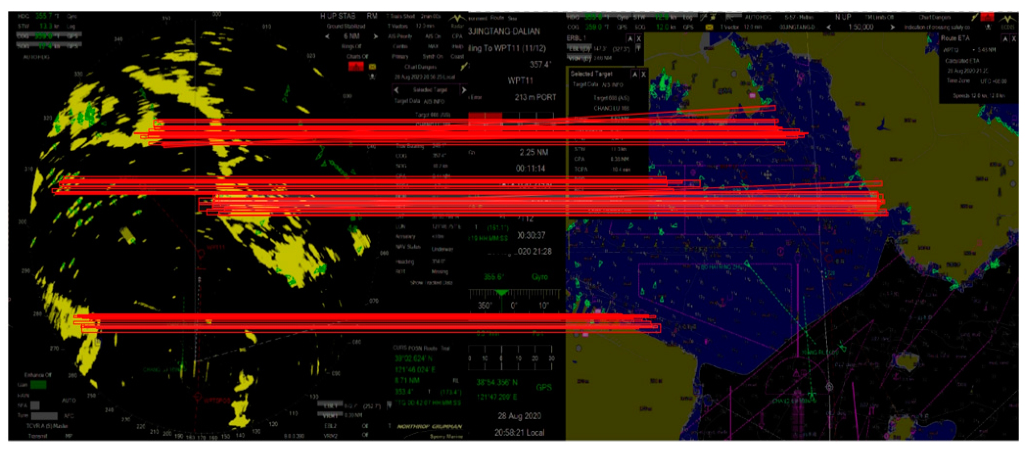
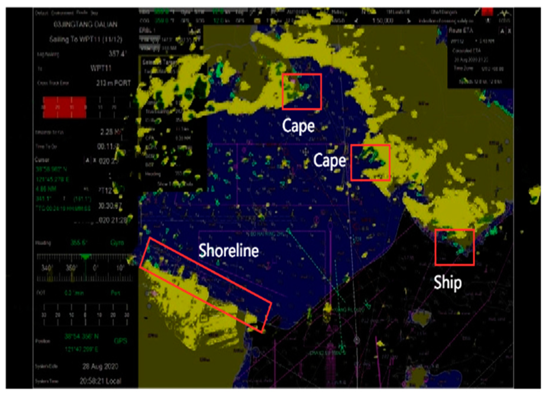
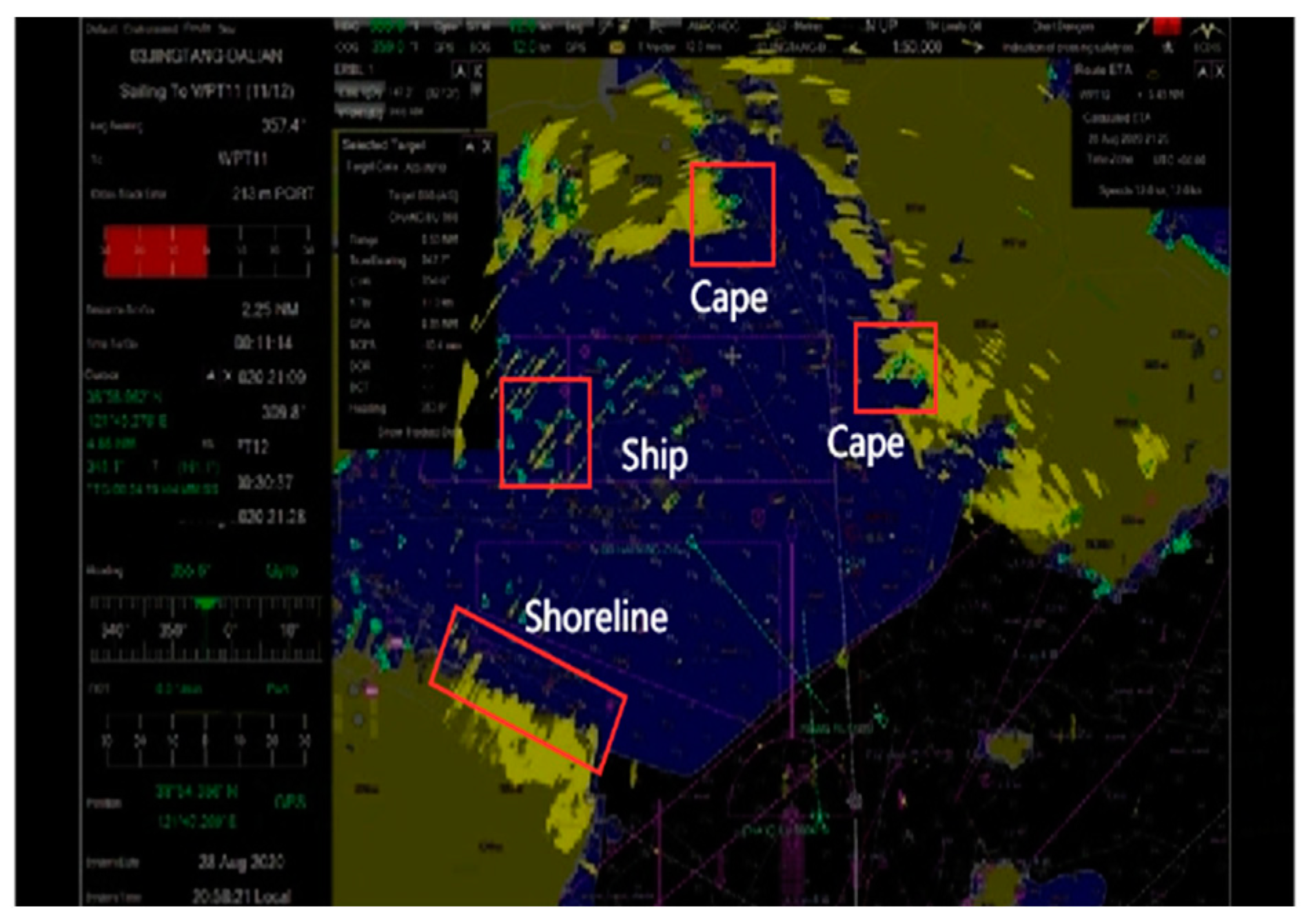
Image fusion is the most important tool for explaining image quality and verifying whether the data obtained by this method are functional or high-resolution. Considering the stage of fusion image and the degree of information extraction, the radar echo image and electronic chart image are fused. A total of 50 groups of electronic charts and navigation radar images are selected for experiments. According to the theory, Y* is the image set that has been fused between electronic charts and navigation radar images, and D* is the marine radar images and electronic charts that have completed the first three steps of image processing. In the filter stage, the high and low resolution filters are set to 8 × 8 × 45. The dictionary learning model optimization process includes two parameters, namely λ and the number of iterations, it is found through many experiments that when λ ϵ [1, 30], there is no significant impact on the image fusion results. Therefore, the parameters are set in this experiment λ = 15. According to the error analysis of dictionary learning, the maximum number of iterations of this experiment is set to 20. The results are shown in Figure 13 and Figure 14. Among them, in order to facilitate identification, the AIS target green triangle of the ship is retained.

Figure 13.
Radar image and electronic chart fusion image before ship turning.
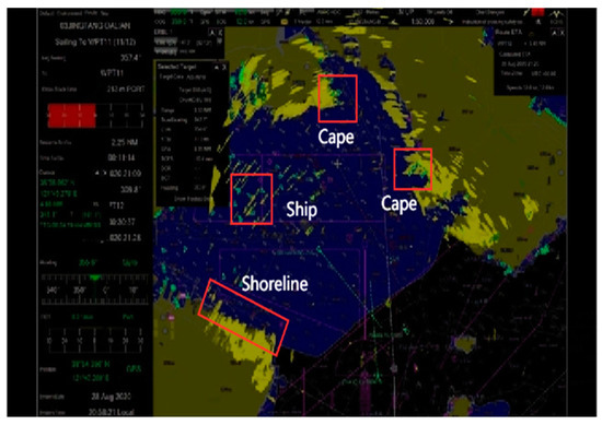
Figure 14.
Radar image and electronic chart fusion image during ship turns.
It can be seen from the image fusion results that the coastline after the fusion of electronic chart and radar echo image data has high consistency, indicating that the algorithm has good performance. Therefore, the automatic fusion algorithm realizes the automatic fusion of electronic chart and radar echo image.
5.4. Image Fusion Quality Evaluation
Corner Overlap (CO) [30] multi-focus image fusion quality evaluation index was used to evaluate the fusion image of radar echo image and electronic chart. The method of Smallest Univalue Segment Assimilating Nucleus (SUSAN) is adopted to detect the corner points in the radar echo image and fusion image. Firstly, the neighborhood that has similarity to the detected corner points is found, and the number and threshold of pixels in the neighborhood are then determined. If the pixel number in the neighborhood is less than the corner point, the detected pixel belongs to the corner point, otherwise it is not the corner point.
The fused images of radar echo image and electronic chart are evaluated by the CO evaluation method, Image Visual Information Fidelity (IVIF) index and Piella index. The Piella index mainly includes a structural similarity theory evaluation index (Qo) and weighted quality evaluation index (Qw). The evaluation outcomes are shown in Table 4.
Table 4.
Objective evaluation index table of fusion.
From the data in the table, the fusion effect of the image fusion method used in this research is more ideal.
6. Conclusions
In order to realize the effective perceptual fusion of ship navigation radar and electronic chart, this research uses Wasserstein distance as the evaluation parameter between distribution and perceptual loss. This research uses the diversity of the radar echo image in the feature space established by perceptual loss calculation to suppress noise. Secondly, a registration method based on image conversion is proposed. By applying the visual attribute transfer algorithm to image conversion, the imaging difference between the images is eliminated, and the registration of the radar echo image and electronic chart image is realized. The electronic chart and radar echo image are then fused by sparse theory and FFT, and the real ship verification is carried out. The image fused by the electronic chart and radar echo image can provide real-time information of marine radar echo, can better reflect the navigational environment of electronic chart, and can thus enhance navigation safety.
Although the design and implementation of the fusion display system can operate normally and realize the basic functions, the fusion system is relatively large because the system contains radar echo images and electronic charts, and some details need to be improved. Moreover, the fusion display of radar echo images and electronic charts and the fusion depth can be further improved to minimize the interference of echo.
Author Contributions
Conceptualization, C.Z., R.Y. and M.F.; methodology; M.F.; validation, C.Z., T.L. and C.Y.; writing—original draft preparation, C.Z., R.Y.; funding acquisition, T.L. All authors have read and agreed to the published version of the manuscript.
Funding
This work was financially supported by the National Nature Science Foundation of China (grant # 51939001, 61976033); the Science and Technology Innovation Funds of Dalian (Grant # 2018J11CY022); the LiaoNing Revitalization Talents Program (Grant # XLYC1908018, XLYC1807046).
Acknowledgments
We are very grateful to the reviewers for their valuable comments that helped to improve the paper.
Conflicts of Interest
The authors declare no conflict of interest.
References
- Zhang, C.; Cao, C.; Guo, C.; Li, T.; Guo, M. Navigation multisensor fault diagnosis approach for an unmanned surface vessel adopted particle-filter method. IEEE Sens. J. 2021, 1, 1–8. [Google Scholar] [CrossRef]
- Abbasi, A.; Monadjemi, A.; Fang, L.; Rabbani, H.; Zhang, Y. Three-dimensional optical coherence tomography image denoising through multi-input fully-convolutional networks. Comput. Biol. Med. 2019, 108, 1–8. [Google Scholar] [CrossRef] [PubMed] [Green Version]
- Goodfellow, I.; Pouget-Abadie, J.; Mirza, M.; Xu, B.; Warde-Farley, D.; Ozair, S.; Courville, A.; Bengio, Y. Generative adversarial networks. Adv. Neural Inf. Process. Syst. 2014, 3, 2672–2680. [Google Scholar] [CrossRef]
- Dong, C.; Loy, C.C.; He, K.; Tang, X. Image super-resolution using deep convolutional networks. IEEE Trans. Pattern Anal. Mach. Intell. 2016, 38, 295–307. [Google Scholar] [CrossRef] [PubMed] [Green Version]
- Zhang, J.; Ma, W.; Wu, Y.; Jiao, L. Multimodal remote sensing image registration based on image transfer and local features. IEEE Geosci. Remote. Sens. Lett. 2019, 16, 1210–1214. [Google Scholar] [CrossRef]
- Meng, Y.; Zhang, Z.; Yin, H.; Ma, T. Automatic detection of particle size distribution by image analysis based on local adaptive canny edge detection and modified circular Hough transform. Micron 2018, 106, 34–41. [Google Scholar] [CrossRef] [PubMed]
- Zhang, D.H.; Zhang, Y.J.; Zhang, C. Faster R-CNN based data fusion of electronic charts and radar images. Syst. Eng. Electron. 2020, 42, 1267–1273. [Google Scholar]
- Li, H.Q.; Yu, Q.C.; Fang, M. Application of Otsu thresholding method on canny operator. Comput. Eng. Des. 2008, 29, 2297–2299. [Google Scholar]
- Liu, Z.; Li, H.; Zhang, L.; Zhou, W.; Tian, Q. Cross-Indexing of Binary SIFT Codes for Large-Scale Image Search. IEEE Trans. Image Process. 2014, 23, 2047–2057. [Google Scholar] [CrossRef]
- Zhou, Z.; Wu, Q.M.J.; Wan, S.; Sun, W.; Sun, X. Integrating SIFT and CNN Feature Matching for Partial-Duplicate Image Detection. IEEE Trans. Emerg. Top. Comput. Intell. 2020, 4, 593–604. [Google Scholar] [CrossRef]
- Donderi, D.C.; Mercer, R.; Hong, M.B.; Skinner, D. Simulated Navigation Performance with Marine Electronic Chart and Information Display Systems (ECDIS). J. Navig. 2004, 57, 189–202. [Google Scholar] [CrossRef]
- Liu, W.T.; Ma, J.X.; Zhuang, X.B. Research on radar image & chart graph overlapping technique in ECDIS. Navig. China 2005, 62, 59–63. [Google Scholar]
- Yang, G.L.; Dou, Y.B.; Zheng, R.C. Method of image overlay on radar and electronic chart. J. Chin. Inert. Technol. 2010, 18, 181–184. [Google Scholar]
- Guo, M.; Guo, C.; Zhang, C.; Zhang, D.; Gao, Z. Fusion of ship perceptual information for electronic navigational chart and radar images based on deep learning. J. Navig. 2020, 73, 192–211. [Google Scholar] [CrossRef]
- Vishwakarma, A.; Bhuyan, M.K. Image fusion using adjustable non-subsampled shearlet transform. IEEE Trans. Instrum. Meas. 2019, 68, 3367–3378. [Google Scholar] [CrossRef]
- Yang, Q.; Yan, P.; Zhang, Y.; Yu, H.; Shi, Y.; Mou, X.; Kalra, M.K.; Zhang, Y.; Sun, L.; Wang, G. Low-dose CT image denoising using a generative adversarial network with wasserstein distance and perceptual loss. IEEE Trans. Med. Imaging. 2018, 37, 1348–1357. [Google Scholar] [CrossRef]
- Ma, X.; Hu, S.; Liu, S.; Fang, J.; Xu, S. Multi-focus image fusion based on joint sparse representation and optimum theory. Signal Process. Image Commun. 2019, 78, 125–134. [Google Scholar] [CrossRef]
- Chen, L.; Qu, H.; Zhao, J.; Chen, B.; Principe, J.C. Efficient and robust deep learning with Correntropy-induced loss function. Neural Comput. Appl. 2016, 27, 1019–1031. [Google Scholar] [CrossRef]
- He, K.M.; Zhang, X.Y.; Ren, S.Q.; Sun, J. Deep residual learning for image recognition. In Proceedings of the IEEE Conference on Computer Vision and Pattern Recognition (CVPR), Las Vegas, NV, USA, 27–30 June 2016; Volume 90, pp. 770–778. [Google Scholar]
- Hu, S.; Zhang, H. Image edge detection based on FCM and improved canny operator in NSST domain. In Proceedings of the 2018 14th IEEE International Conference on Signal Processing (ICSP), Beijing, China, 12–16 August 2018; pp. 363–368. [Google Scholar]
- Bai, X.; Peng, X. Radar image series denoising of space targets based on gaussian process regression. IEEE Trans. Geosci. Remote. Sens. 2019, 57, 4659–4669. [Google Scholar] [CrossRef]
- Liao, J.; Yao, Y.; Yuan, L.; Hua, G.; Kang, S.B. Visual attribute transfer through deep image analogy. ACM Trans. Graph. 2017, 36, 1–15. [Google Scholar] [CrossRef] [Green Version]
- Yuan, L.; Zhao, Q.; Gui, L.; Cao, J. High-dimension tensor completion via gradient-based optimization under tensor-train format. Signal. Process. Image Commun. 2018, 73, 53–61. [Google Scholar] [CrossRef]
- Elhamifar, E.; Vidal, R. Sparse subspace clustering: Algorithm, theory, and applications. IEEE Trans. Pattern Anal. Mach. Intell. 2013, 35, 2765–2781. [Google Scholar] [CrossRef] [PubMed] [Green Version]
- Kircheis, M.; Potts, D. Direct inversion of the nonequispaced fast Fourier transform. Linear Algebra its Appl. 2019, 575, 106–140. [Google Scholar] [CrossRef] [Green Version]
- Kreutz-Delgado, K.; Murray, J.F.; Rao, B.D.; Engan, K.; Lee, T.-W.; Sejnowski, T.J. Dictionary learning algorithms for sparse representation. Neural Comput. 2003, 15, 349–396. [Google Scholar] [CrossRef] [PubMed] [Green Version]
- El Helou, M.; Susstrunk, S. Blind universal bayesian image denoising with gaussian noise level learning. IEEE Trans. Image Process. 2020, 29, 4885–4897. [Google Scholar] [CrossRef] [Green Version]
- Chen, H.; Zhang, Y.; Kalra, M.K.; Lin, F.; Chen, Y.; Liao, P.; Zhou, J.; Wnag, G. Low-dose CT with a residual encoder-decoder convolutional neural network (RED-CNN). IEEE Trans. Med. Imaging 2017, 36, 2524–2535. [Google Scholar] [CrossRef]
- Li, Z.; Shi, W.; Xing, Q.; Miao, Y.; He, W.; Yang, H.; Jiang, Z. Low-dose CT image denoising with improving WGAN and hybrid loss function. Comput. Math. Methods Med. 2021, 13, 10435–10440. [Google Scholar]
- Anselmo, M.; Giammarresi, D.; Madonia, M. Sets of pictures avoiding overlaps. Int. J. Found. Comput. Sci. 2019, 30, 875–898. [Google Scholar] [CrossRef]


Publisher’s Note: MDPI stays neutral with regard to jurisdictional claims in published maps and institutional affiliations. |
© 2021 by the authors. Licensee MDPI, Basel, Switzerland. This article is an open access article distributed under the terms and conditions of the Creative Commons Attribution (CC BY) license (https://creativecommons.org/licenses/by/4.0/).