The Close Relationship between Internal Wave and Ocean Free Surface Wave

Abstract

A numerical model was used to simulate the propagation of internal waves (IW) along the surface layer. The results show that strong water exchange during IW propagation results in strong free surface flow and produces small but distinct free surface waves. We found a close relationship between the internal and ocean surface waves. Our intuitive reaction is that by training the relationship between the water surface wave height and the internal wave waveform, the internal wave waveform can be reversed from the water surface wave height value. This paper intends to validate our intuition. The artificial neural network (ANN) method was used to train the Fluent simulated results, and then the trained ANN model was used to predict the inner waves below by the free surface wave signal. In addition, two linear internal wave equations (I and II) were derived, one based on the Archimedes principle and the other based on the long wave and Boussinesq approximation. The prediction by equation (II) was superior to the prediction of equation (I), which is independent of depth. The predicted IW of the proposed ANN method was in good agreement with the simulated results, and the predicted quality was much better than the two linear wave formulas. The proposed simple method can help researchers infer the magnitude of IW from the free surface wave signal. In the future, the spatial distribution of IW below the sea surface might be obtained by the proposed method without costly field investigation.

1. Introduction

Internal waves (IW) occur along the boundaries of different seawater densities, which will result in changes in the pressure gradient. Internal waves are a large number of water movements within the ocean that can have a profound impact on ecosystems, offshore engineering facilities, commercial and military vessels, and even the climate. In recent years, related research has become increasingly popular, and a large number of reports on field investigations have been published. Early field investigations included [1,2,3,4]. However, in early field investigations, data was limited by single-point observations, and measurement data did not provide large spatial information. With the development of satellite remote sensing technology and synthetic aperture radar (SAR), researchers can use visible light images to interpret surface roughness and light reflection intensity, and then indirectly describe internal waves [5] analyzed the image data of synthetic aperture radar, the field observation data of conductivity, temperature, and depth (CTD), acoustic Doppler current profiler (ADCP), and EK-500 scientific echo sounder system, and reported the distribution map of internal waves, but the detailed amplitude of the following internal waves was not notified.

Furthermore, the weather conditions, cost, and safety have restricted the application of site investigation of the internal waves. Many researchers started using lab experiments in the internal wave studies, such as [1,6,7,8]. The suggestions given by [9] became the basis of the later experimental studies, since they considered that wave shape parameters and their results agree well with the KDV theory.

High computation performance can be achieved even in a personal computer; researchers began to develop numerical model to study the internal waves, such as [10,11,12,13]. The advantages of low cost and space have drawn more attention of researchers using numerical methods to study internal wave propagations. [14] showed that the wave-induced sea surface displacements could be the indicators of the presence of internal waves, and they also suggested that the surface information may be used in the context of the internal wave analysis if the surface displacements are captured with sufficient precision. More databases have become available recently, such as [15,16].

In recent years, the researchers use high-resolution remote sensing instruments such as synthetic aperture radar (SAR) to survey internal wave images of relatively larger areas. Figure 1 shows an SAR image of an internal wave around Korea [17]. In a satellite image, we generally assume the white color indicates crests of waves on the ocean surface and dark color indicates troughs of waves. Hajji et al. [18] reported an operational system based on SAR image analysis and a hydrodynamic model for simulating the internal waves generated by barotropic tides on a continental shelf. They assumed that the imaging mechanism can be well interpreted with the modulation surface variation according to tide driving current. Besides, the internal wave motion also induces surface current and will regulate surface wave spectrum and the image intensity, as well. However, the SAR observations are not frequently sampled, and the data obtained by SAR do not make it easy to produce the required detailed quantitative results because the data obtained from space range over a relatively large area which is too coarse. Kropfli et al. [19] used shore-based microwave radars as the assistant observation tools and analyzed the relationships between internal waves and their radar and radiometric signatures. Based on the data obtained by the radars, they can describe the IWs effects on short gravity capillary waves, which strongly modulate the radar signals. The relationships were analyzed between oceanic isotherm vertical displacements, internal currents, and radar backscatter cross sections, along with airship-measured Doppler velocity signals and temperatures. Hong et al. [20] reported an analysis of internal waves around the Korean Peninsula using RADARSAT-1 data. They found that the surface signatures of oceanic internal waves (IWs) can be observed in synthetic aperture radar (SAR) images because IWs could change surface roughness through the interaction of small-scale ocean waves with varying currents induced by IWs. Once the relationship between the vertical and horizontal parameters governing IWs is established, the mixed-layer depth (MLD) can be estimated from SAR data.

In our study, we also found that divergence and convergence do occur as depression and elevation IW passing below the surface. The existence of close relationship between free surface perturbation and internal wave propagation were also found previously [18,19,21]. In the later sections of the paper, we use the trained artificial neural networks (ANNs) model to correlate the free surface wave displacements and the interfacial displacements. The trained ANN model is used to predict interface variation by the free surface wave signals. Although the remote sensing images could not deduce the amplitudes and the types of the internal waves traveling below, the free surface wave characteristics can be deduced by SAR [17]. Therefore, once the free surface heights can be obtained by SAR image, the proposed trained ANN model may possibly produce the hindcasting of the internal wave below.

In the present study, a commercial code. Fluent (ANSYS). was used to simulate IW passing the horizontal sea bottom. Section 2 briefly describes the equations of motion of fluid and the boundary conditions used by Fluent. The numerical techniques used by ANSYS Fluent are also introduced in this section. This section introduces a brief description of the ANN method used in the study. Section 3 discusses the development, propagation, and dissipation mechanisms of the internal waves. The relationship between free surface wave and internal wave is analyzed to find a close relationship between internal wave and surface wave. In addition, in this section, the ANN method is used to train the simulated results of free surface waves and internal waves. The trained ANN model is, then, used to predict internal wave below by the simulated free surface wave (as input signals). The linear internal wave theory is introduced and the comparison of IW prediction by ANN method and linear IW theory is made in this section. The final concluding remarks are given in Section 4.

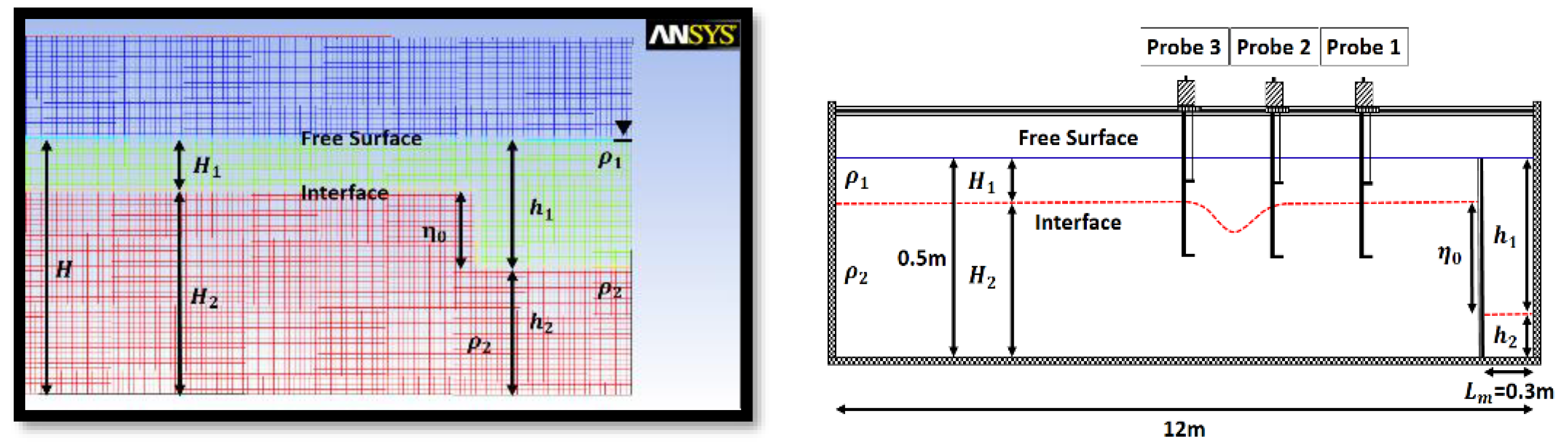
2. Numerical Method

In this section, the numerical method and ANN method were briefly described.

2.1. Fluent Simulation Method

A commercial code, Fluent 6.3, is used in the study. The governing equations used are the Navier-Stokes equations along with the continuity equation, and they are solved to acquire the velocity and pressure fields. The continuity equation is

$$\frac{\partial \mathrm{u}}{\partial \mathrm{x}}+\frac{\partial \mathrm{w}}{\partial \mathrm{z}}=0$$

(1)

The Navier-Stokes equations of a 2D incompressible flow can be written as

$$\frac{\partial \mathrm{u}}{\partial \mathrm{t}}+\mathrm{u}\frac{\partial \mathrm{u}}{\partial \mathrm{x}}+\mathrm{w}\frac{\partial \mathrm{u}}{\partial \mathrm{z}}=-\frac{1}{\mathsf{\rho }}\frac{\partial \mathrm{P}}{\partial \mathrm{x}}+\frac{\mathsf{\mu }}{\mathsf{\rho }}\left(\frac{{\partial }^2\mathrm{u}}{\partial {\mathrm{x}}^2}+\frac{{\partial }^2\mathrm{u}}{\partial {\mathrm{z}}^2}\right)$$

(2)

$$\frac{\partial \mathrm{w}}{\partial \mathrm{t}}+\mathrm{u}\frac{\partial \mathrm{w}}{\partial \mathrm{x}}+\mathrm{w}\frac{\partial \mathrm{w}}{\partial \mathrm{z}}=-\frac{1}{\mathsf{\rho }}\frac{\partial \mathrm{P}}{\partial \mathrm{z}}+\frac{\mathsf{\mu }}{\mathsf{\rho }}\left(\frac{{\partial }^2\mathrm{w}}{\partial {\mathrm{x}}^2}+\frac{{\partial }^2\mathrm{w}}{\partial {\mathrm{z}}^2}\right)-\mathrm{g}$$

(3)

where t is the time and u and w are, respectively, the velocity components in x and z direction, p is the pressure, $\mathsf{\rho }$ is the fluid density, and $\mathsf{\mu }$ is the dynamic viscous coefficient. Two types of fluid are used in the study, one is air and the other is liquid, which have upper and lower layers with different densities of 998.2 kg/m³ and 1030 kg/m³, respectively. The sea surface is an interface between air and liquid, and the pressure-inlet with standard temperature and pressure are given to model the air–sea interface. The volume of fluid (VOF) method [22] is used to trace and locate the instant sea–air interface and interface between two liquid layers. The stagger grid is used. The discretization techniques used are the quadratic upwind interpolation of convective kinematics (QUICK) method [23] and the pressure implicit with splitting of operator (PISO) algorithm [24] as the iteration techniques to solve for flow velocity as well as the pressure fields. For obtaining better accuracy of the results, the second-order upwind scheme is used.

The mesh arrangement and the definition sketch of the computational domain are depicted in Figure 2. The locations of three probes are 5.7 L_m, 9 L_m, and 12.3 L_m, respectively. A gravity collapse method is used to generate the solitary wave. The numerical wave tank is set as L = 12 m, the wave generated area is L_m = 0.3 m, the water depth H = H₁ + H₂ = 0.7 m, and the potential difference [25,26,27] at the wave generated area is η_o = 30 cm.

The numerical analysis methods and numerical results validations are basically reported in the previous paper [21]. The numerical results are compared with reported experimental data. They reported the comparison of the Fluent simulated results with experimental data. The experimental data were provided by Chen [28], and in Chen’s experiment, the ultrasonic probes (LEGI, Institute National Polytechnique de Grenoble, France) recorded the interface fluctuations, and the electrical capacitance gauges (developed by NCKU) recorded the free surface displacements. We set a computational domain the same as the setup of the experiments made by Chen and compared our simulated results of the interfacial displacement at the location of the probes in the experiment with the measured data of Chen’s experiments. The detailed numerical procedures are described in Chen et al. [21] and are omitted in this paper. The simulated IWs generated in the numerical tank with different water layers thicknesses are then used to set up the ANN model for IW hindcasting and validation.

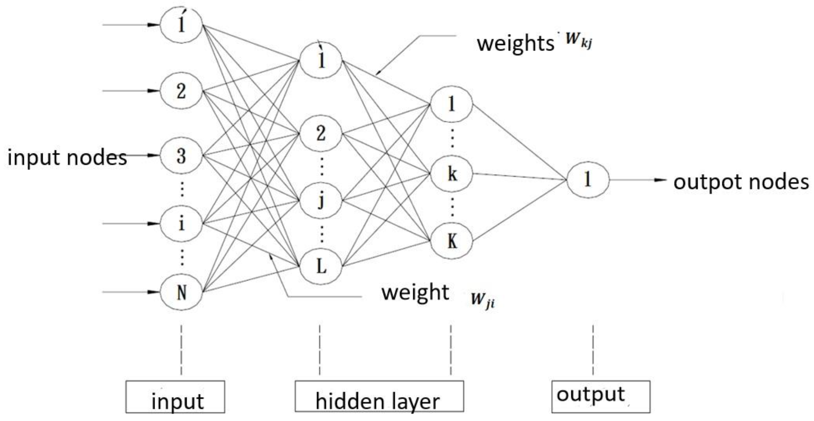
2.2. Artificial Neural Network (ANN)

The artificial neural network (ANN) model is applied in many different scientific fields [29]. From the general definition, this model can be treated as a special form of statistic technique. It can effectively deal with data regression and simulate the nonlinear system and time series problem. An artificial neural network is defined as a structure composed of a number of interconnected units or artificial neurons. Each unit has input/output (I/O) characteristics and implements a local computation or function. The output of any unit is determined by its I/O, its interconnection to other units, and possibly external inputs. The back propagation (BP) network is most popularly used, and it consists of at least three layers of units: an input layer, intermediate hidden layer, and an output layer. The detailed algorithm can be found elsewhere (such as [30]) and is omitted in the text. In many real-world situations, the data might be incomplete or noisy, and it is important to be able to make reasonable predictions about what is missing from the information available. The artificial neural network-back propagation (ANN-BP) model has been applied to tidal forecasting and data supplement (such as [30]). A BP network consists of at least three layers of units: an input layer, intermediate hidden layer, and an output layer (see Figure 3). Typically, these units are connected in a feed-forward manner where the input units are completely connected to units in the hidden layer and hidden units are also completely connected to units in the output layer. The layers consist of many processing elements that can simulate biological neurons. The hidden layers are the special characteristic of this ANN-BP model. Because of this characteristic, the nonlinear system and time series problem can be simulated. A description of the theory of the ANN model can be found in [30] and is omitted here.

The time (t), free surface wave height (${\mathsf{\eta }}_{\mathrm{fs}}$), and upper and lower water depths (${\mathrm{H}}_1$) and (${\mathrm{H}}_2$), are set as the data used in the input layers, and the amplitude of IW (${\mathsf{\eta }}_{\mathrm{iw}}$) is set as the data used in the output layer. We chose the results of the 17 simulations as the trained data and those of the remained simulation as the verification data. The evaluation index used is the root mean squared errors, RMSE, which can be given as

$$\mathrm{RMSE}=\sqrt{\frac{1}{\mathrm{n}}\times {\displaystyle \sum }_{\mathrm{i}=1}^{\mathrm{n}}{\left({\mathrm{T}}_{\mathrm{i}}-{\mathrm{A}}_{\mathrm{i}}\right)}^2}$$

(4)

where n is sample numbers, ${\mathrm{T}}_{\mathrm{i}}$ is ith observed data, and ${\mathrm{A}}_{\mathrm{i}}$ is the predicted data. The Pearson correlation coefficient, R, is used to evaluate the correlation between observed and verification (or predicted) data, and the Pearson correlation coefficient is expressed as

$$\mathrm{R}=\frac{{\displaystyle \sum }\left({\mathrm{T}}_{\mathrm{i}}-\overline{\mathrm{T}}\right)\left({\mathrm{A}}_{\mathrm{i}}-\overline{\mathrm{A}}\right)}{\sqrt{{\displaystyle \sum }{\left({\mathrm{T}}_{\mathrm{i}}-\overline{\mathrm{T}}\right)}^2}\sqrt{{\displaystyle \sum }{\left({\mathrm{A}}_{\mathrm{i}}-\overline{\mathrm{A}}\right)}^2}}$$

(5)

where $\overline{\mathrm{T}}$ is the mean observed data and $\overline{\mathrm{A}}$ is the average output data. The observed and predicted data have high correlation if $\left|\mathrm{R}\right|>0.7$, intermediate correlation when $0.3\le \left|\mathrm{R}\right|\le 0.7$, and low correlation if $\left|\mathrm{R}\right|<0.3$. The Pearson correlation coefficient is used later, in Section 3.3, to see the correlation between ANN predicted results and Fluent simulated results.

3. Results and Discussion

In this section, we firstly presented the simulation of an IW passing a planar sea bottom and delineated and confirmed the relationship between the evolution of an IW and the displacement of the surface wave patterns. In the later sections, the artificial neuron network (ANN) model is used to train the simulated displacements of free surface wave and the interfacial elevation of the water layers at a specific probe location, and the trained ANN model is, then, used to predict the elevation of an IW at a specific location by the simulated free surface wave height at the same location.

3.1. IW Propagation

The depression and elevation waves are defined by Maxworthy [31] according to the thickness ratio ζ = (H₁/H₂) of the upper to the lower water layers. When the ratio ζ is less than or larger than 1, the depression and elevation waves will occur, respectively. Accompanied by the propagation of the IW, the transient free surface flow is generated, and the IW will also create vortices and alter the amplitude and the period of the surface waves. The moving direction of the water above the interface of an elevation wave is opposite to wave direction, whereas the water below the interface has the same moving direction as the wave, and an opposite phenomenon occurs in the case of a depression IW propagation.

The simulation cases made in this study are listed in

Table 1. Parameters used in different cases [21].

Cases	${\mathbf{H}}_1/{\mathbf{H}}_2$	${\mathbf{h}}_1/{\mathbf{h}}_2$	${\mathsf{\eta }}_0\left(\mathbf{cm}\right)$
Case-A	10/40 (depression)	15/35, 20/30, 25/35	5, 10, 15
Case-B	15/35 (depression)	20/30, 25/25, 30/20	5, 10, 15
Case-C	20/30 (depression)	25/25, 30/20, 35/15	5, 10, 15
Case-D	40/10 (elevation)	35/15, 30/20, 25/25	5, 10, 15
Case-E	35/15 (elevation)	30/20, 25/25, 20/30	5, 10, 15
Case-F	30/20 (elevation)	25/25, 20/30, 15/35	5, 10, 15

. Six upper and lower water layers depth ratios ζ and three water potential η₀ at the wave maker area (WMA) are used. In the wave maker area, each case has three different water depth ratios, i.e., there are three different elevation heads of each case and we have totally simulated 18 cases.

After carefully studying the displacement of the free surface wave and the variation of the internal wave elevation, we found a close relationship between the free surface displacement and the interface profile. Figure 4 shows the time history of free surface wave displacement and interface height at Probe-2. Regardless of the type of IW, free surface displacement and interface height will change in different trends. In the main part of the IW, as the depressions and elevation waves pass below, the free surface rises and sinks, respectively [21]. The figure clearly demonstrates that the free surface is pooling down at the front area of the leading edge of a depression IW and is heaving at the main portion of a depression IW. 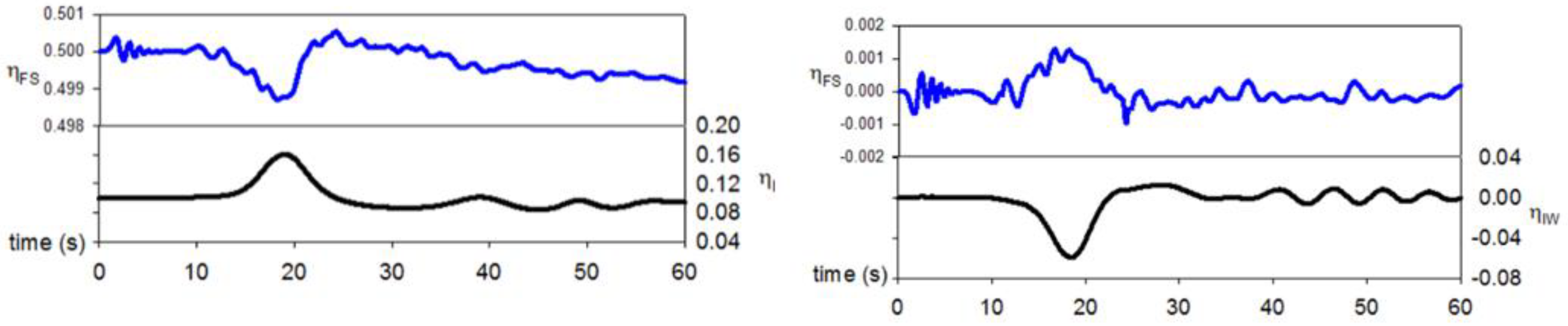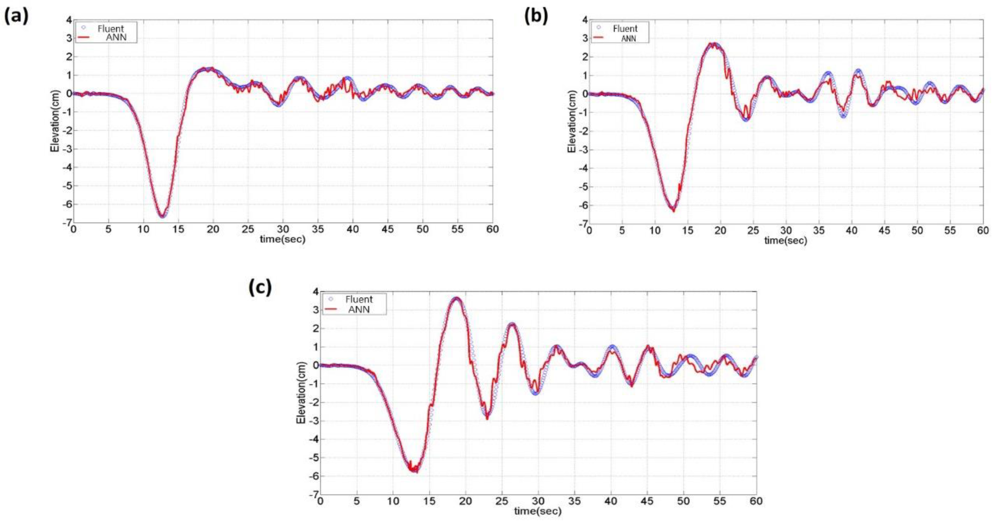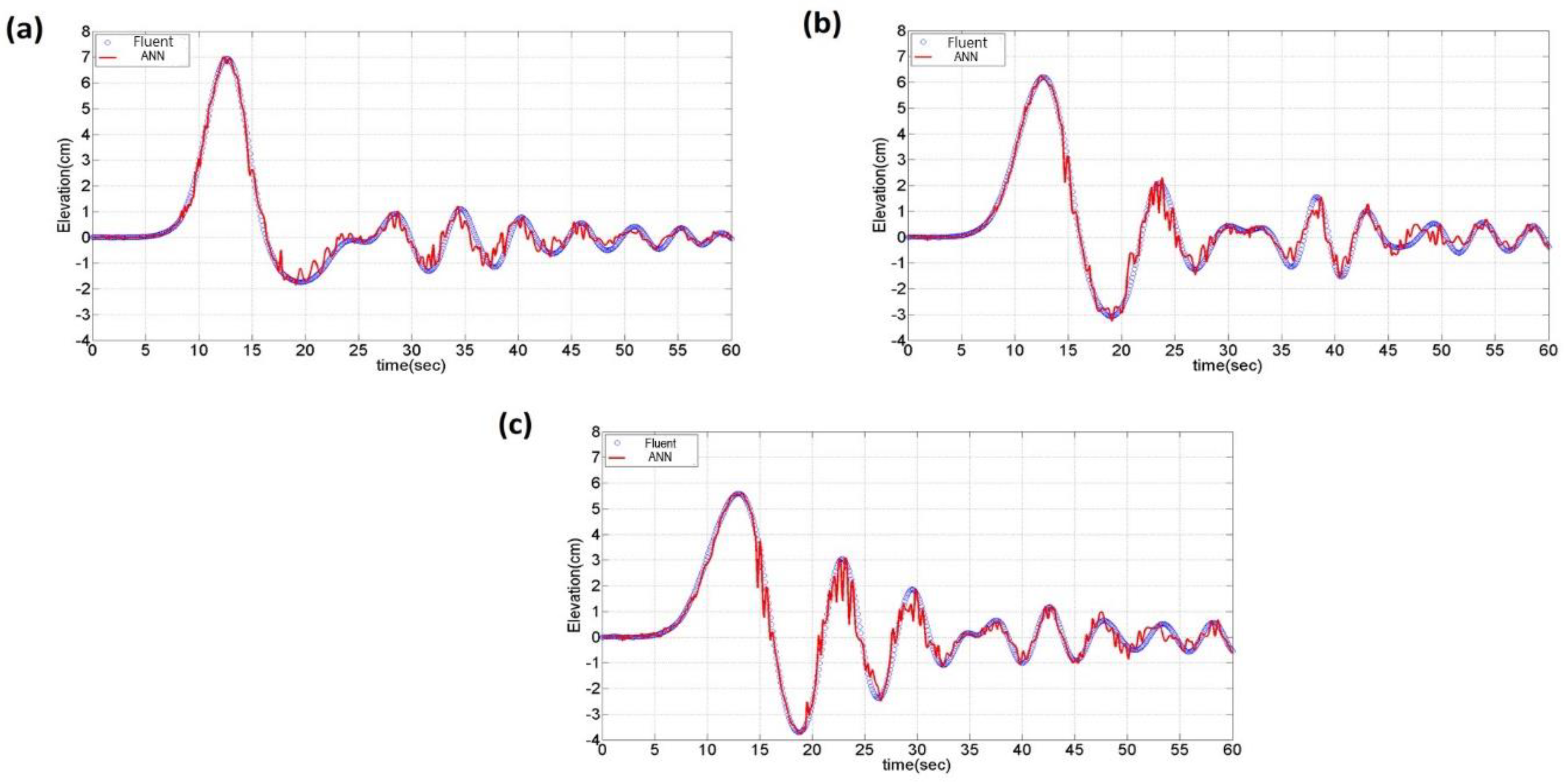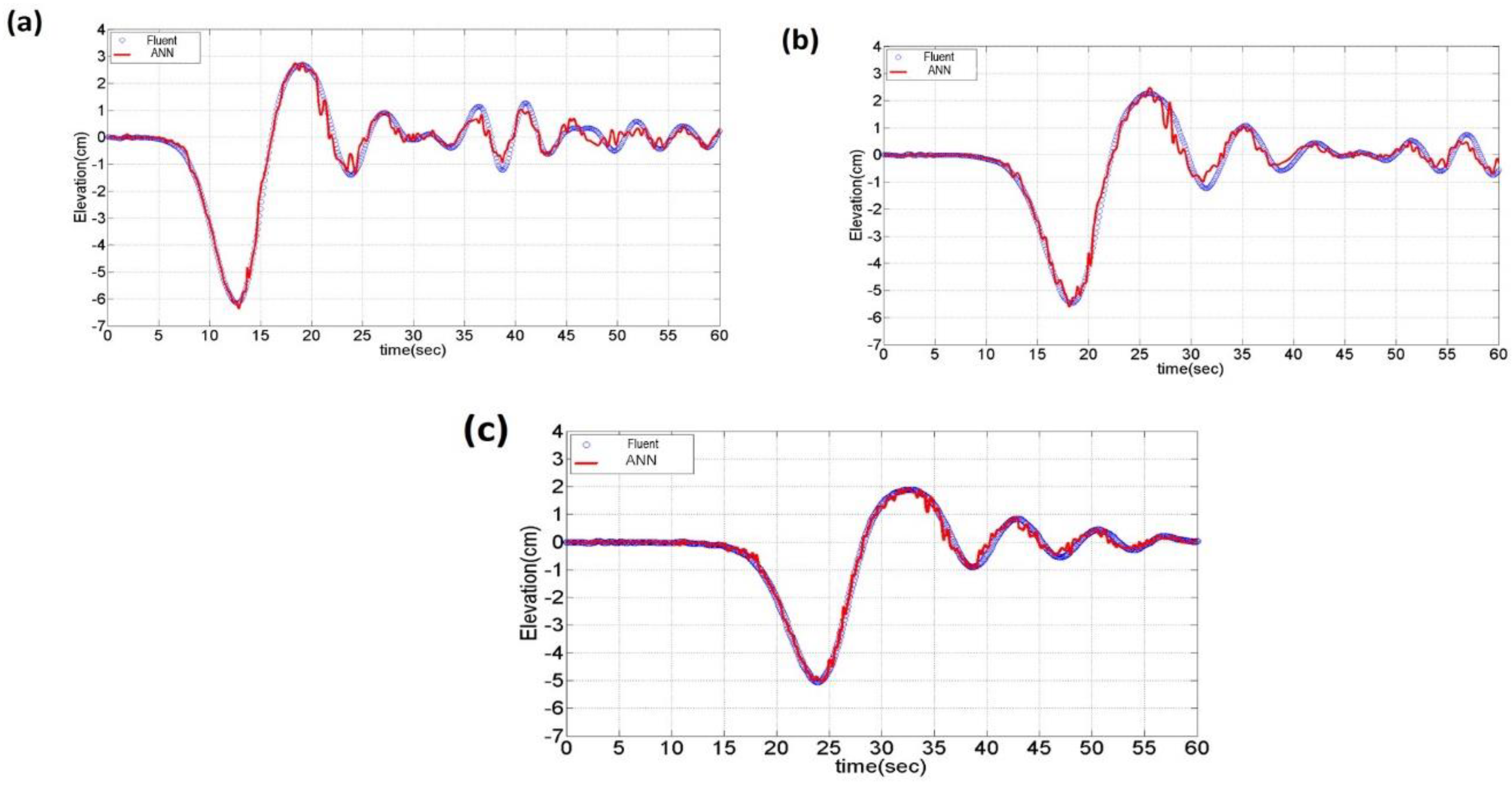The opposite displacement trends of the free surface are found in the cases of an elevation wave propagation.

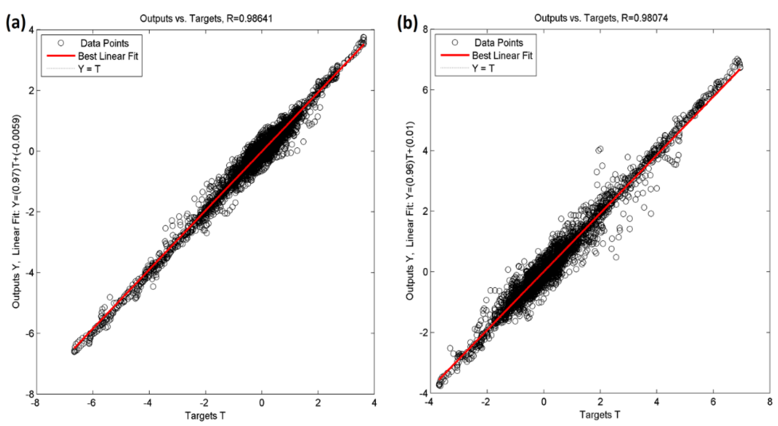
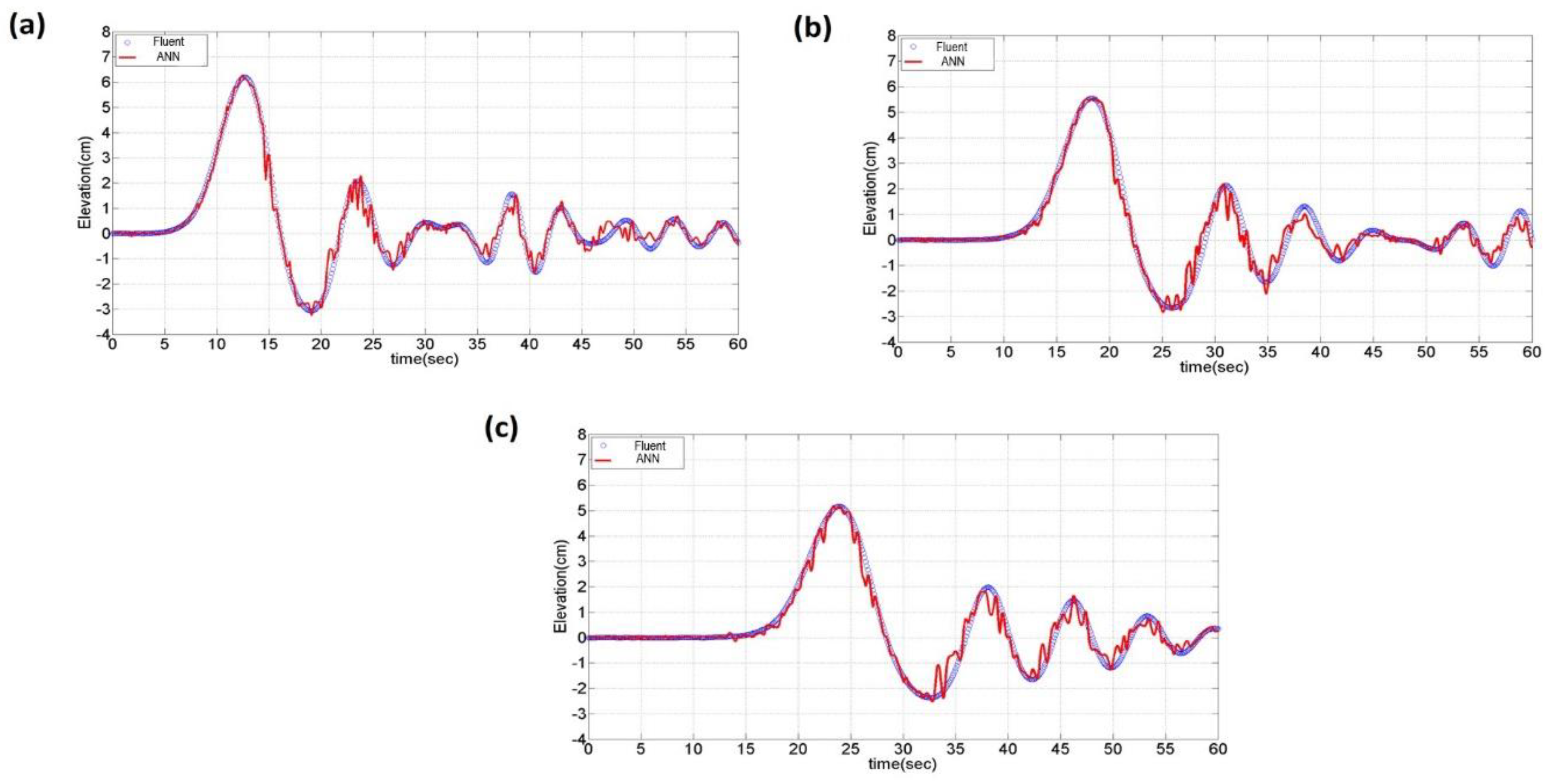
3.2. Correlation between the Simulated and ANN Predicted IWs

The number of the hidden layers will affect the precision of the ANN model, and the proper numbers of the hidden layers are determined by parametric tests.

Table 2. The RMSE and correlation coefficient R with various numbers of hidden layers.

	Depression Wave Cases		Elevation Wave Cases
Numbers of Hidden Layers	RMSE	R	RMSE	R
25	0.3111	0.9680	0.4116	0.9480
50	0.2386	0.9813	0.3105	0.9708
100	0.2088	0.9857	0.2826	0.9758
150	0.2037	0.9864	0.2526	0.9807

shows that the RMSE decreases and the correlation coefficients increase as the number of the hidden layers increases. Figure 5 further shows the correlation between simulated data by Fluent and the ANN predicted data of cases A and D. As depicted in the figure, the correlation is very good; the correlation coefficients R (0.986 and 0.981) of both cases are greater than 0.98, which implies that correlations between simulated and predicted data are very high.

IW Prediction by Free Surface Wave Signals

The trained ANN model was used to predict the variation of IW. The simulated free surface wave data of different cases were recorded, and they were used as input data of the ANN model, and the trained ANN model will give predicted IW. Figure 6 depicts the comparison between simulated and predicted data at Probe-1. The comparisons of three different cases are shown in the figure, and the predicted data agrees very well with the simulated data, especially in the time period where the main IW passes Probe-1 and a minor difference occurs when the trailing waves pass. Figure 7 shows the comparison of the interfacial displacement of an elevation internal wave and the agreement between ANN predicted and ANSYS simulated results is also very good. Figure 8 and Figure 9 further compare the simulated results and predicted data of cases B and E at three different probes, and the agreements between predicted and simulated data are also very good. Similar to the results shown in Figure 6 and Figure 7, the ANN-predicted primary IWs agree nearly perfect well with simulated results, and the relatively larger discrepancy occurs in the trailing waves. Better agreements between simulated and ANN-predicted results for trailing waves can be found in the case of Probe-3, which is further away from the vertical gate and the gravity collapse disturbance is less than those of Probes 1 and 2.

The results listed in Table 2 and the plots shown in Figure 6, Figure 7, Figure 8 and Figure 9 give us solid confidence to believe the ANN method can be used to predict spatial variation of IW by using free surface observation data. The remote sensing images may provide the information of the surface wave heights of a large area. Although the free surface wave heights are much less than the amplitude of the IW below, the proposed ANN method successfully made the hindcasting of the amplitude of interfacial profile by using relatively much smaller free surface wave heights. Most recently, Shao et al. [32] used C-band VV-polarization Sentinel-1 synthetic aperture radar (SAR) imagery data, and a semi-empirical algorithm successfully retrieved significant wave height (Hs) and mean wave period. Once the free surface wave heights are remotely readable, the proposed ANN method presented in the paper can be associated with the remote sensing radar (such as synthetic aperture radar, SAR) to predict the spatial variation of the internal wave passing below.

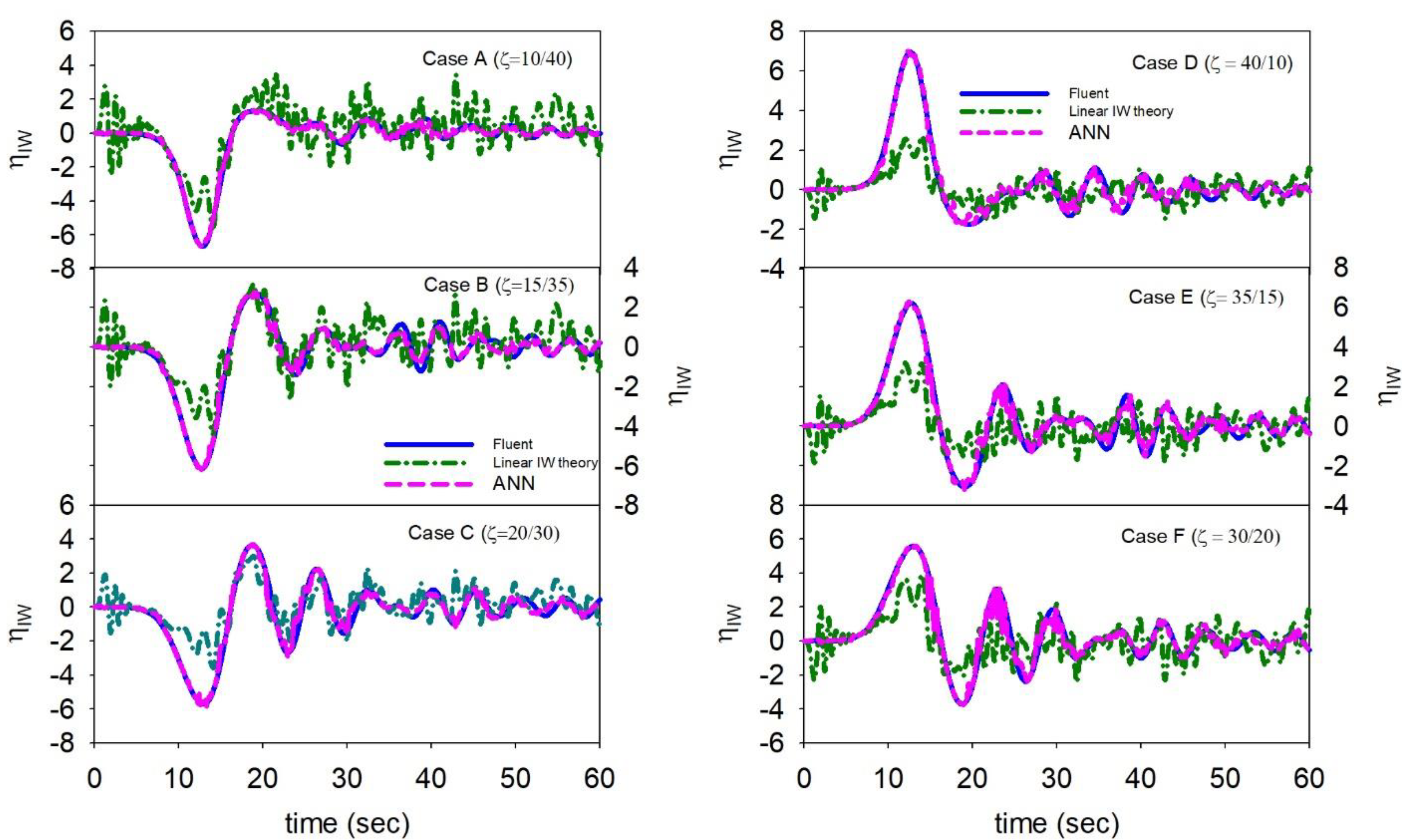
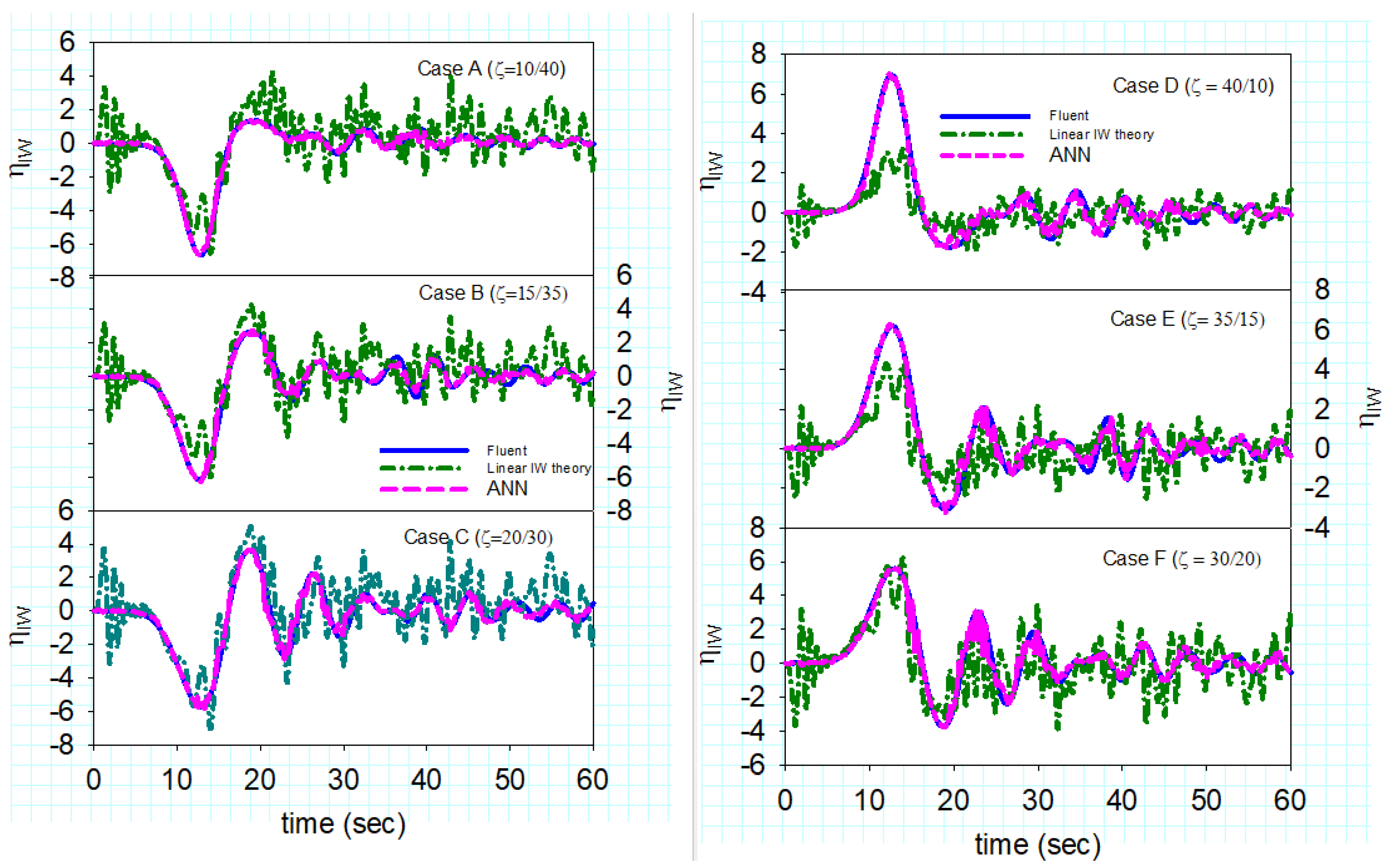
3.3. Linear Internal Wave Theory

Two linear internal wave theories were considered in this study: Linear wave theory I is based on Archimedes principle, and Linear wave theory II is considered depth effect and Boussinesq approximation [16,18,19].

3.3.1. Linear Wave Theory I: (Archimedes Principle)

According to Archimedes principle, the weight of an immersed object is reduced by the weight of fluid it displaces. Assuming two layers of fluid, the pressure in the second layer can be derived and given as

$$p_2={\rho }_{1}g({\eta }_1-{\eta }_2)+{\rho }_2\mathrm{g}({\eta }_2-z)$$

(6)

where η₁ and η₂ are, respectively, the free surface elevation and layer interface elevation. Suppose that the layer of fluid (fluid 1) is lying on a denser layer of fluid (fluid 2) and the lower fluid is assumed to be always in equilibrium, i.e., ∂_xp = ∂_yp = 0. Thus, we have

$${\partial }_x{p}_2={\rho }_{1}g({\partial }_x{\eta }_1-{\partial }_x^{}{\eta }_2)+{\rho }_2\mathrm{g}{\partial }_x{\eta }_2=0$$

(7)

and comes to

$${\eta }_1=-\frac{{\rho }_2-{\rho }_1}{{\rho }_1}{\eta }_2$$

(8)

According to Equation (8), in the ocean, the gravity is reduced from −2.5% g to −3% g. The free surface can be −2.5% to −3% oppositely perturbed by the internal wave. Based on the simulated internal wave displacement, the simple equations described above give an estimate of the free surface displacement: Figure 10 depicts the free surface disturbance displacement, and the Fluent simulated displacement is also shown in the figure. The solid line is the result of Fluent, and the dotted line is evaluated by Equation (8), which is based on linear wave theory I. We can see that the shapes of the free surface displacements are substantially the same, but the magnitude and position of the valleys of the free surface waves are different from each other. In other words, the linear IW theory I cannot correctly predict the amplitude of the free surface wave and the arrival time of the IW.

Figure 11 further compares the interfacial displacement and simulated data at Probe-1 in six different cases obtained by the ANN method and the linear IW theory I. It can be seen from the figure that the interface displacement predicted by ANN is in good agreement with the observations in all six cases, while the linear IW theory I can only predict the trend of interface displacement; however, the prediction quality is much worse than that of the ANN method.

3.3.2. Linear Wave Theory II: (Depth Effects Included)

In the linear wave theory I, the depth effects were not included, and they might affect the relationship between free surface wave and interfacial waves. To consider the depth effects, we may assume a two-layer fluid in the linear long-wave approximation; the following formula can be given [33]:

$${\eta }_1=\left(\frac{c^2}{c^2-g{H}_1}\right){\eta }_2$$

(9)

where c is phase speed of the linear long-wave. For an internal wave, c² < gH₁, and so we obtain the well-known opposite polarity of the surface displacement to the interface displacement. If the internal speed is approximate using the Boussinesq approximation, that is $c^2\approx \frac{g({\rho }_2-{\rho }_1)}{{\rho }_2}\frac{H_1{H}_2}{H_1+H_2}$ and then we obtain the new linear wave formula as

$$\frac{{\eta }_1}{{\eta }_2}\approx -\frac{{\rho }_2-{\rho }_1}{{\rho }_2{H}_1+{\rho }_1{H}_2}{H}_2$$

(10)

Equation (10) shows that this linear wave formula has a dependence on the fluid layer depths. Figure 12 compares the predicted IW by ANN method and the new linear wave formula, and the prediction based on the new linear formula (Equation (10)) is still worse than that of ANN method; however, the quality of the prediction is much better than that based on Equation (8), which is not depth-dependent.

3.4. The Layers Thickness Prediction

In this section, we define ξ as the ratio of the interfacial displacement to free surface displacement, that is, $\xi ={\eta }_2/{\eta }_1$. The simulated results of this study also indicate that ζ = H₁/H₂ and ξ have a close relationship. Figure 13 depicts the relationship among layers thicknesses and the ratio of free surface displacement to interfacial displacements. As shown in the figure, there is a linear relationship between the layer thickness ratio ζ and the ratio of interfacial displacement to free surface displacement ξ. For the depression IWs and elevation IWs, we have the following regression formulae, respectively,

$$\zeta =-0.1314\xi -3.285$$

(11)

and

$$\zeta =-0.184\xi -0.00187{\xi }^2-3.858$$

(12)

We can use the free surface displacement to predict the interface displacement and calculate the ratio of the two displacements and use the above two equations to determine the layer thickness ratio, and then the upper and lower layer thicknesses can be obtained.

4. Conclusions

The gravity collapse method was used in a CFD code ANSYS Fluent to generate the IWs. The numerical validations of the Fluent simulated results were made, and the CFD code was then used to simulate 18 IWs generation cases, including both depression and elevation IWs. The simulated results show that the propagation of the trough or peak of IW will trigger the transient free surface flow, and that the free surface displacement was affected by the rotating flow in the upper water layer. The simulated IWs generated in the numerical tank with different water layers thicknesses were made in [21], and the simulated results were then used to set up the ANN model for IW hindcasting and validation. The following concluded remarks can be given:

(1)

The simulated data were used to train an ANN model which was used to predict the IWs profile by the free surface displacement. The comparisons of three different depression IWs propagation cases show that the predicted data agrees very well with the simulated data, especially in the time period of main IW passes Probe-1, and minor difference occurs when the trailing waves pass. Similar behaviors were found in the elevation IWs propagation cases.

(2)

The comparison of ANN-predicted IWs and those predicted by linear IW theory was also made. The hindcasting quality of ANN-predicted IWs are very good, whereas the prediction made by the linear IW theory without depth effect can only give correct trend of the interfacial displacement. The prediction accuracy is poor, and the arrival time lag is also found in the prediction of linear wave theory I. As the depth effects were considered, the prediction quality of the linear wave theory became better, especially in depression IWs prediction.

(3)

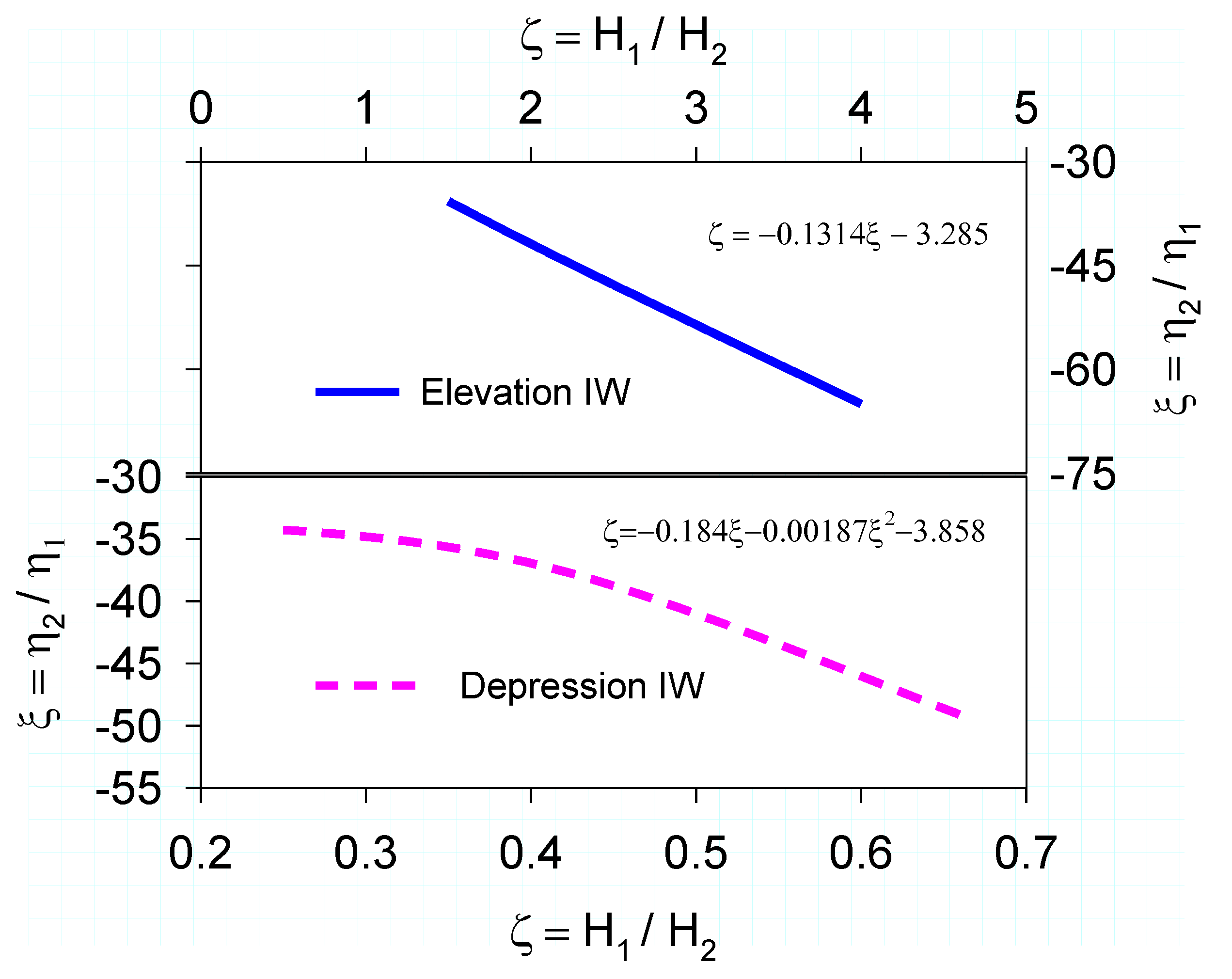
The simple formulae are given for layer thickness ratio prediction. We may use simulated free surface displacement to predict the interfacial displacement and calculate the ratio of both displacements and use the regression equations to determine the layers thickness ratio, and the upper and lower layer thicknesses can then be obtained.

(4)

In addition, the relationships between free surface displacement and layers thickness ratio are also determined. The observed maximum peak and minimum trough displacements of the free surface wave can be used to calculate the layers thickness ratio, and the depths of the upper and lower water layers can be easily determined.

(5)

Using the free surface wave signal observed by a remote buoy, the proposed ANN model is applicable and can successfully predict the spatial variation of the internal wave. Thus, the proposed simple method may help researchers to infer the amplitude of IW from remote surface wave signatures. In the future, the spatial distribution of IW below the sea surface might be obtained by the proposed method without costly field investigation.

References

- Thrope, S.A. The excitation, dissipation, and interaction of internal waves in the deep ocean. J. Geophys. Res. 1975, 80, 328–338. [Google Scholar] [CrossRef]
- Cairns, J.L.; Williams, G.O. Internal wave observations from a midwater float, 2. J. Geophys. Res. 1976, 81, 1943–1950. [Google Scholar] [CrossRef]
- Farmer, D.M. Observation of long nonlinear internal waves in a lake. J. Phys. Oceanogr. 1978, 8, 63–73. [Google Scholar] [CrossRef] [Green Version]
- Osborne, A.R.; Burch, T.L. Internal solitons in the Andaman Sea. Science 1980, 208, 451–460. [Google Scholar] [CrossRef]
- Ebbesmeyer, C.C.; Romea, R.D. Final Design Parameters for Solitons at Selected Locations in South China Sea; Final and Supplementary Reports Prepared for Amoco Production Company: Houston, TX, USA, 1992; 209p. [Google Scholar]
- Benjamin, T.B. Internal waves of finite amplitude and permanent form. J. Fluid Mech. 1966, 25, 241–270. [Google Scholar] [CrossRef] [Green Version]
- Benjamin, T.B. Internal waves of permanent form in fluids of great depth. J. Fluid Mech. 1967, 29, 559–592. [Google Scholar] [CrossRef]
- Ono, H. Algebraic solitary waves in stratified fluid. J. Phys. Soc. Jpn. 1975, 39, 1082–1091. [Google Scholar] [CrossRef]
- Koop, C.G.; Butler, G. An investigation of internal solitary waves in a two-fluid system. J. Fluid Mech. 1981, 112, 225–251. [Google Scholar] [CrossRef]
- Muller, P.; Liu, X. Scattering of internal waves at finite topography in two dimensions. Part I: Theory and case studies. J. Phys. Oceanogr. 2000, 30, 532–549. [Google Scholar] [CrossRef]
- Vlasenko, V.; Hutter, K. Numerical experiments on the breaking of solitary internal waves over a slope-shelf topography. J. Phys. Oceanogr. 2002, 32, 1779–1793. [Google Scholar] [CrossRef]
- Grimshaw, R.; Pelinovsky, E.; Taipova, T. Rogue internal waves in the ocean: Long wave model. Eur. Phys. J. Spec. Top. 2010, 185, 195–208. [Google Scholar] [CrossRef]
- Nycander, J. Generation of internal waves in the deep ocean by tides. J. Geophys. Res. 2005, 110, C10028. [Google Scholar] [CrossRef] [Green Version]
- Álvarez, Ó.; González, C.J.; Mañanes, R.; López, L.; Bruno, M.; Izquierdo, A.; Gómez-Enri, J.; Forero, M. Analysis of short-period internal waves using wave-induced surface displacement: A three-dimensional model approach in Algeciras Bay and the Strait of Gibraltar. J. Geophys. Res. 2011, 116, C12033. [Google Scholar] [CrossRef] [Green Version]
- Epifanova, A.S.; Rybin, A.V.; Moiseenko, T.E.; Kurkina, O.E.; Kurkin, A.A.; Tyugin, D.Y. Database of Observations of the Internal Waves in the World Ocean. Phys. Oceanogr. 2019, 26, 350–356. [Google Scholar] [CrossRef] [Green Version]
- Noh, S.; Nam, S. Observations of enhanced internal waves in an area of strong mesoscale variability in the southwestern East Sea (Japan Sea). Sci. Rep. 2020, 10, 9068. [Google Scholar] [CrossRef]
- NASA. Earth Sciences and Image Analysis Laboratory. Date Acquired: 24 January 2020, Courtesy of NASA. Available online: https://www.jpl.nasa.gov/spaceimages/details.php?id=PIA01915 (accessed on 24 January 2020).
- Hajji, H.; Sole, S.; Ramamonjiarisoa, A. Analysis and Prediction of Internal Waves Using SAR Image and Non-Linear Model. In Proceedings of the a SAR Workshop: CEOS Committee on Earth Observation Satellites, Working Group on Calibration and Validation, Toulouse, France, 26–29 October 1999. [Google Scholar]
- Kropfli, R.A.; Ostrovski, L.A.; Stanton, T.P.; Skirta, E.A.; Keane, A.N.; Irisov, V. Relationships between strong internal waves in the coastal zone and their radar and radiometric signatures. J. Geophy. Res. 1999, 104, 3133–3148. [Google Scholar] [CrossRef]
- Hong, D.-B.; Yang, C.-S.; Kim, T.-H.; Ouchi, K. Analysis of internal waves around the Korean Peninsula using RADARSAT-1 data. In Proceedings of the SPIE 9240, Remote Sensing of the Ocean, Sea Ice, Coastal Waters, and Large Water Regions 2014, Amsterdam, The Netherlands, 22–25 September 2014. [Google Scholar] [CrossRef]
- Chen, B.-F.; Huang, Y.-J.; Chen, B.; Tsai, S.-Y. Surface wave disturbance during internal wave propagation over various types of sea bottoms. Ocean. Eng. 2016, 125, 214–225. [Google Scholar] [CrossRef]
- Hirt, C.W.; Nichols, B.D. Volume of fluid (VOF) method for the dynamics of free boundaries. J. Comput. Phys. 1981, 39, 201–225. [Google Scholar] [CrossRef]
- Leonard, B.P. A stable and accurate convective modelling procedure based on quadratic upstream interpolation. Comput. Methods Appl. Mech. Eng. 1979, 19, 59–98. [Google Scholar] [CrossRef]
- Issa, R.I. Solution of the implicitly discretised fluid flow equations by operator-splitting. J. Comput. Phys. 1986, 62, 40–65. [Google Scholar] [CrossRef]
- Hsieh, C.M.; Hwang, R.R.; Hsu, J.R.C.; Cheng, M.H. Numerical modeling of flow evolution for an internal solitary wave propagating over a submerded ridge. Wave Motion 2015, 55, 48–72. [Google Scholar] [CrossRef]
- Fu, K.S. The Effect of Nonlinearity and Mixed Layer Thickness on the Propagation of Nonlinear Internal Waves. Master’s Thesis, Institute Physical Oceanography, National Sun Yat-sen University, Kaohsiung, Taiwan, 2007. (In Chinese). [Google Scholar]
- Kuo, C.F. The Experimental Study of IW Pass an Obstacle. Master’s Thesis, Institute of Institute Physical Oceanography, National Sun Yat-sen University, Kaohsiung, Taiwan, 2005. (In Chinese). [Google Scholar]
- Chen, S.H. The Experimental Study of IW over a Slope Sea Bed. Master’s Thesis, Department of Marine Environment and Engineering, National Sun Yat-sen University, Kaohsiung, Taiwan, 2004. (In Chinese). [Google Scholar]
- Malekmohamadia, I.; Ghiassia, R.; Yazdanpanahb, M.J. Wave hindcasting by coupling numerical model and artificial neural networks. Ocean. Eng. 2008, 35, 417–425. [Google Scholar] [CrossRef]
- Chen, B.F.; Wang, H.D.; Chu, C.C. Wavelet and artificial neural network analyses of tide forecasting and supplement of tides around Taiwan and South China Sea. Ocean. Eng. 2007, 34, 2161–2175. [Google Scholar] [CrossRef]
- Maxworthy, T. A note on the internal solitary waves produced by tidal flow over a three-dimensional ridge. J. Geophys. Res. 1979, 84, 338–346. [Google Scholar] [CrossRef]
- Shao, W.; Zhang, Z.; Li, X.; Li, H. Ocean Wave Parameters Retrieval from Sentinel-1 SAR Imagery. Remote Sens. 2016, 8, 707. [Google Scholar] [CrossRef] [Green Version]
- Magic Lectures on Nonlinear Waves. Available online: http://www.maths.dept.shef.ac.uk/magic/course.php?id=21 (accessed on 24 January 2020).