Article

Fractal Dimension as an Effective Feature for Characterizing Hard Marine Growth Roughness from Underwater Image Processing in Controlled and Uncontrolled Image Environments

1
Research Institute of Civil Engineering and Mechanics (GeM), Sea and Littoral Research Institute (IUML), Université de Nantes, CNRS UMR 6183/FR 3473, 44300 Nantes, France
2
IXEAD, CAPACITES Society, 44000 Nantes, France
3
QUANT Group, Department of Civil, Structural and Environmental Engineering, Trinity College Dublin, Dublin 2, Ireland
4
Dynamical Systems and Risk Laboratory, UCD Centre for Mechanics, School of Mechanical and Materials Engineering, University College Dublin, Dublin 4, Ireland
5
Science Foundation Ireland MaREI Centre, University College Dublin, Dublin 4, Ireland
6
The Energy Institute University College Dublin, Dublin 4, Ireland
7
Science Foundation Ireland Connect Centre, Trinity College Dublin, Dublin 4, Ireland
8
Laboratoire de Recherche en Hydrodynamique, Énergétique et Environnement Atmosphérique (LHEEA), Sea and Littoral Research Institute (IUML), Ecole Centrale de Nantes, CNRS UMR 6598/FR 3473, 44300 Nantes, France
*
Author to whom correspondence should be addressed.
J. Mar. Sci. Eng. 2021, 9(12), 1344; https://doi.org/10.3390/jmse9121344
Submission received: 15 October 2021 / Revised: 8 November 2021 / Accepted: 9 November 2021 / Published: 29 November 2021
(This article belongs to the Special Issue Underwater Computer Vision and Image Processing)

Abstract

:
Hard marine growth is an important process that affects the design and maintenance of floating offshore wind turbines. A key parameter of hard biofouling is roughness since it considerably changes the level of drag forces. Assessment of roughness from on-site inspection is required to improve updating of hydrodynamic forces. Image processing is rapidly developing as a cost effective and easy to implement tool for observing the evolution of biofouling and related hydrodynamic effects over time. Despite such popularity; there is a paucity in literature to address robust features and methods of image processing. There also remains a significant difference between synthetic images of hard biofouling and their idealized laboratory approximations in scaled wave basin testing against those observed in real sites. Consequently; there is a need for such a feature and imaging protocol to be linked to both applications to cater to the lifetime demands of performance of these structures against the hydrodynamic effects of marine growth. This paper proposes the fractal dimension as a robust feature and demonstrates it in the context of a stereoscopic imaging protocol; in terms of lighting and distance to the subject. This is tested for synthetic images; laboratory tests; and real site conditions. Performance robustness is characterized through receiver operating characteristics; while the comparison provides a basis with which a common measure and protocol can be used consistently for a wide range of conditions. The work can be used for design stage as well as for lifetime monitoring and decisions for marine structures, especially in the context of offshore wind turbines.

1. Introduction

Within a short period of time after construction, offshore structures are usually covered with a biofilm, which serves for the development of macrofouling. Some key effects of marine growth on offshore structures have been investigated several decades back [1,2,3] and include bio-chemical attacks in the form of corrosion effects, masking effect for structural inspections, mass effect related to structural over-loading, and hydrodynamic over-loading effect related to drag (e.g., flow through screens).
Generally, biofouling can be divided into hard (mussels, barnacles, oysters), soft (anemones, soft corals, seaweeds), and long flapping (kelps) categories. Biofouling can reach a considerable extent depending on the site location and water depth [2,4,5]. Additionally, it is well known since the 1970s that one of the main drivers for hydrodynamic changes is the roughness of hard marine growth and that long flapping kelps change the dynamic behavior through vortex induced vibrations [6]. The roughness turbulence generated by all the different types of fouling are dissimilar [7]. Roughness caused by the presence of hard marine growth (barnacles, oysters, mussels, etc.) is known to change the flux around an immersed cylindric component by changing the frontier between hydrodynamical regimes assessed by the Reynolds number (sub, post-super critical Reynolds numbers) and the hydro-dynamic coefficients of the Morison equation [8,9]. Uncertainties from hydrodynamic and biological parts can be accounted for through response surfaces [10].
In the majority of cases, several types of biofouling communities colonize the surface, but normally there are dominant species and types. Dominant communities and similar species are likely to have similar characteristics in terms of roughness and weight. However, the uncertainty of this characterization is generally high from on-site inspection. Idealization of such growths exists in recommended engineering practices [11,12] in comparison with real shape and distribution. Theophanatos [6] evaluates that the roughness varies between 8–34 mm for a single layer covering of mussels. Following recent investigations and based on more information from site conditions, it is understood that the recommended idealizations of biofouling can often be unrepresentative of real colonization, and the roughness is quite random (Figure 1). A limited number of tests in a tank were carried out with random roughness when it was idealized [6], and, thus, the hazard of biofouling was not fully characterized for (i) analyzing its representativeness of natural colonization, (ii) reproducing the test carried out, or (iii) comparing idealized shapes with other similar shapes used in other tests. In this context, only a few papers simulate the loading on structures in the presence of random roughness [9]. As a consequence, the quantification and modeling of the real shape from on-site inspection is mandatory to better represent the reality and to provide specifications for new tests [13,14].
Progress in recent years has seen improvement in both on-site protocols for thickness assessment and underwater image processing [15,16]. This allows on-site roughness measurements once the protocols are established. Contrary to thickness measurements [17], roughness measurements require low turbidity, and there is a paucity in literature in terms of appropriate features to use.
The requirement of assessment of biofouling has become more relevant in the recent years with the rise of offshore wind turbines to produce renewable energy. Such turbines tend to get bigger with each generation, giving rise to more slender solutions with higher dynamics, nonlinearity, and the impact of secondary loads such as biofouling becoming critical for their lifetime performance. They also contribute to extra fatigue on the structure and on the geotechnical base, which can be crucial when deciding on site reuse following one life cycle of a turbine. With the underwater drone market and their performance in harsh conditions rapidly improved, inspection and maintenance will depend increasingly on image processing and the related assessment, analysis, and interpretation of visual data. Under such circumstances, the gap in choice of appropriate features, testing environment, and quantitative evaluation of the performance of such features and methods under laboratory and real-life conditions are exceedingly important to be established. This paper approaches this problem for hard biological growths, and related detection aspects of surface roughness due to their growth, which guide the unwanted hydrodynamic effects over their lifetime.
To address this, Section 2 focuses on two critical parameters of laboratory and field imaging protocol, the artificial light and the distance to the structure. These are tested first in controlled laboratory conditions for cones of various color, height, and diameter, which is not just a rapid assessment of the imaging protocol but also an assessment of idealistic testing conditions that are often created in scaled wave basin tests. Section 3 implements an established image processing methodology [16] for such laboratory tests, including coupons to optimize the image processing parameters. This follows an automatic segmentation algorithm implementation and the development of indicators of quality of assessment based on detection threshold and quality of sizing. Several estimates for selection of the best protocol are tested and compared, and receiver operating curves are selected. For real inspections where roughness is a random process, methods for roughness quantification are introduced through the fractal dimension. Section 4, in the context of the proposed fractal dimension, demonstrates how to robustly choose testing protocols for site implementation, linking it back to initial laboratory testing framework. This also demonstrates how an overarching experimental protocol can reduce the interpretative gap between realistic biological effects and idealistic laboratory tests or synthetic simulations, which are bound to miss complexities of nature. This protocol is then implemented successfully to the offshore site of Université de Nantes UN-SEA [18], and roughness due to natural colonization of adult mussels along anchoring lines is characterized through its fractal dimension. Data of roughness are then post-processed. The fractal dimension is validated as an appropriate metric for characterizing the on-site complex shape of homogeneous hard biofouling.
The results have an impact on enhancing the value of information from visual inspections [19] and in the testing and monitoring of wind turbines [20,21] and other marine structures. While biofouling is a part of a design process of offshore structures, such structures are often investigated at a low technological readiness level (TRL). Under such circumstances, we need to have better tools and markers, even for a low TRL and for ocean wave basins.

2. Case Studies

Roughness assessment is affected by several environmental factors and experimental conditions, such as wake, luminosity, and turbidity. Wake can be managed by selected sea states for underwater inspection, but both luminosity and turbidity are difficult to forecast and are usually to be dealt with during diving. Laboratory tests were carried out to measure the effect of these parameters on the roughness measurement, with the knowledge that its order of magnitude varies between 8 mm–34 mm for species encountered along European coasts [6]. Refraction may also play an effect, but eventually the light and turbidity combination turns out to be one of the core combinations that also takes into account some of the effects of refraction.

2.1. Underwater Image Acquisition

Underwater images are available from video recordings carried out with Aksi3D protocol (Figure 2a). The objective is to obtain as much benefit as possible from a simple, easy to use, and robust system for providing stereoscopic images. It consists of two synchronized cameras fixed on a T-structure, on which a telescopic jib is fixed in view to control the distance between the cameras and the structure (Figure 2b). This jib is ended with a U-shape tube in view to carry out measurement along chains (Figure 2c). Two GoPro 3 Black edition cameras have been employed with checkerboard calibration. Two waterproof Sola Dive 1200 Light & Motion LED lights were also added with the following set ups, (i) “flood” with a 60-degree angle of flood beam and (ii) “spot” with a 12-degree angle of spot beam (Figure 2b). In both conditions, the maximum capacity of lights (2 × 1200 lumens) have been used. Artificial lighting is preferred in this experiment to ensure the control of operational conditions.

2.2. Artificial Coupon and Test Tank

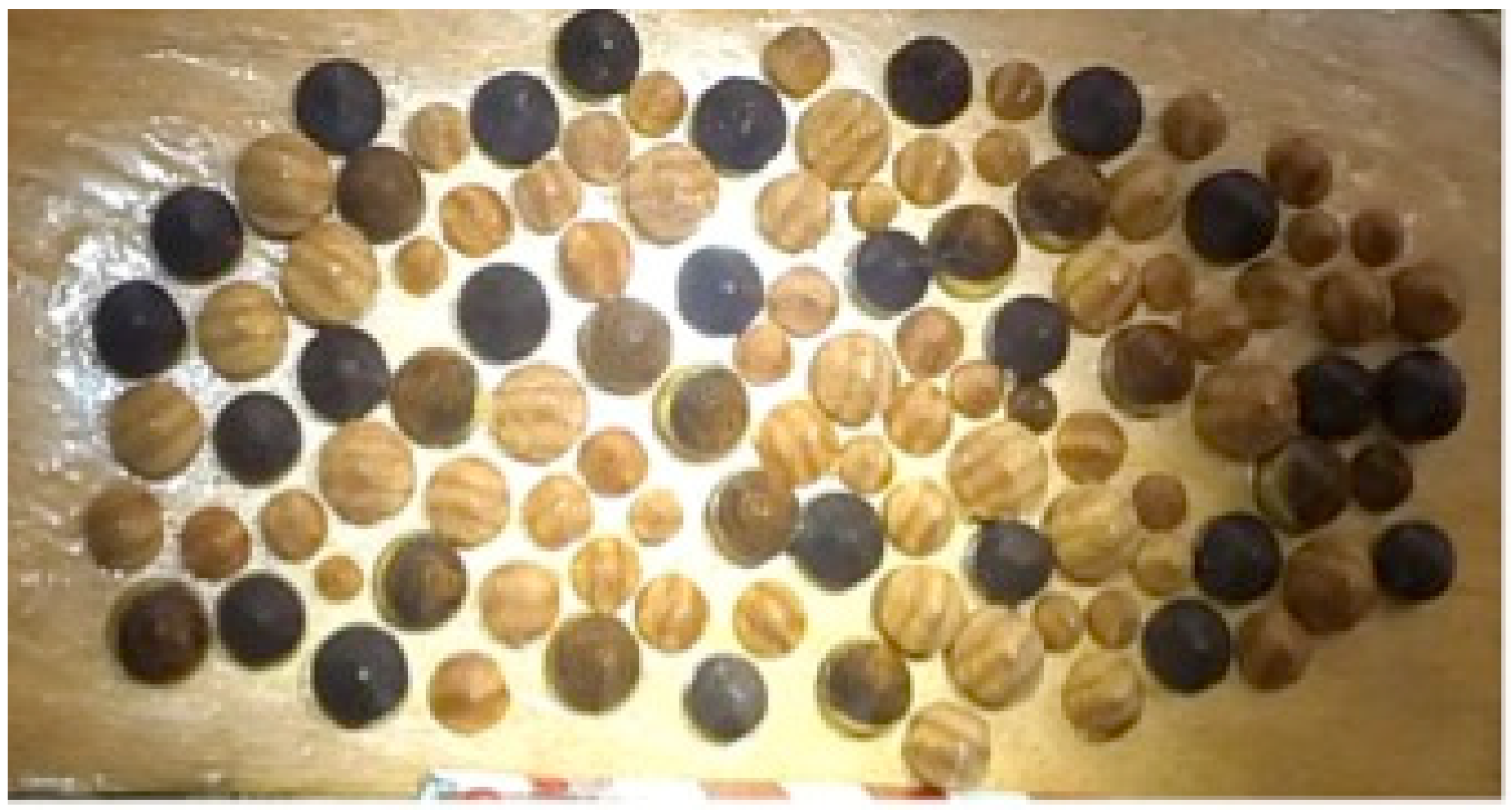
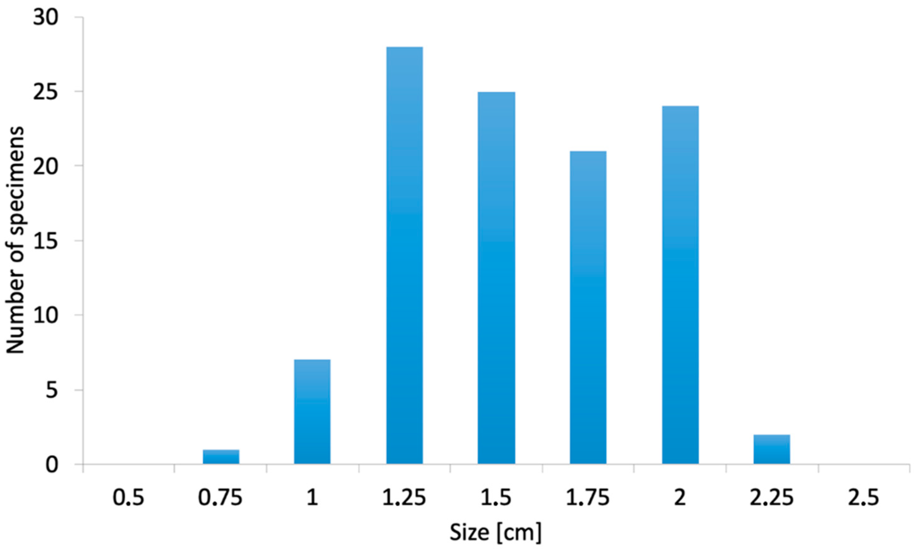
The coupon is an artificially colonized plate built from wood. On this, 108 wood cones of various diameters, heights, and colors were glued. Wood gives a natural variability of colors for each cone and between cones (Figure 3). Each cone and the wood plate were covered by a translucent colored lacquer coating in view to obtain some of the worst conditions for which the light is reflected. Finally, the heights of the specimen were randomly selected between 7 and 21 mm, with a mean value of 14.7 mm and a standard deviation of 3.2 mm. Note that the diameter of the cone’s base depends on each height. Contact between specimens is realistic (barnacles or mussels for instance) and offers the worst conditions for identification of boundaries. The shape was selected because it offers a compromise between the shape of two common species, barnacles (pyramids) and mussels (ellipse).
The distribution of heights is given in Figure 4. Note that, due to the U-shape end of the jib, 13 cones were not visible and were removed from the database for detection (low part Figure 5).
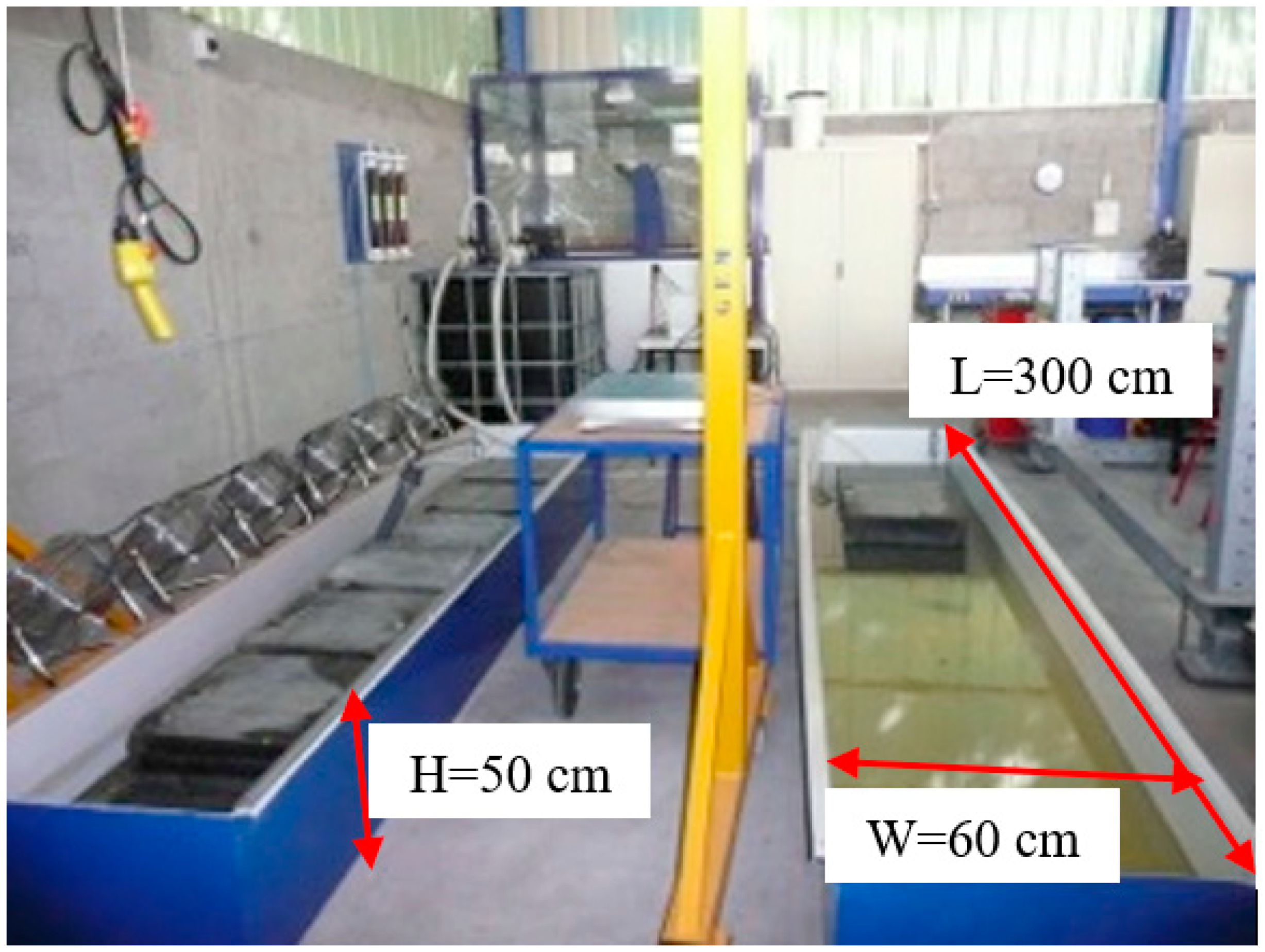
The test tank of Université de Nantes (Figure 6) is a unit of the UN-SEA-Material Durability Testing-Center and is 3 m long, 0.6 m wide, and 0.5 m deep. This tank is used for under-water image processing and tide simulation for material degradation. The wood plate is fixed vertically at one end, and measurements are carried out by placing our device horizontally. Two examples are provided in Figure 5.

2.3. On-Site Measurements

The best protocol selected from tests in the laboratory is used for the measurements carried out on site and is supported by LEHERO-MG project [13,14,22,23,24]. A day and depth were selected, in view to get these conditions, and three pictures on three separated parts of a chain were taken. This chain is the main anchoring material for the equipment buoys of the SEMREV site, operated by Ecole Centrale de Nantes, where adult mussels were observed. The same type of picture was obtained 10 km away, on the test platform UN@SEA (called UN-SEA-SMS previously) [18] of Université de Nantes, two years after its installation in June 2017. The main interest is that the colonization is homogeneous; the chain is fully covered by the same species (the pictures of these mature mussels were taken in 2019). These three pictures are given in Figure 7.
The roughness appears to be slightly different in the three pictures; there can be considered multiple realizations of the stochastic process. The colonization in these pictures is similar (same species and same thickness with the same maturity), and it is known that the arrangement of mussels depends on the available place and the capacity to open the two shells for capturing and filtering water. These pictures will help to highlight if an invariant exists for embracing these realizations. This will be studied by analyzing the ability of statistical and numerical estimates to characterize the roughness of this homogeneous colonization.

3. Isolation of Specimens, Quality of Measurement, and Roughness Mathematical Modeling

The roughness of the chosen specimens was estimated as per API-RP-2A [11]. This means that the distance between the mean surface (here the surface of the wood plate) and the peak (the height of the cone) should be measured.

3.1. Automatic Segmentation

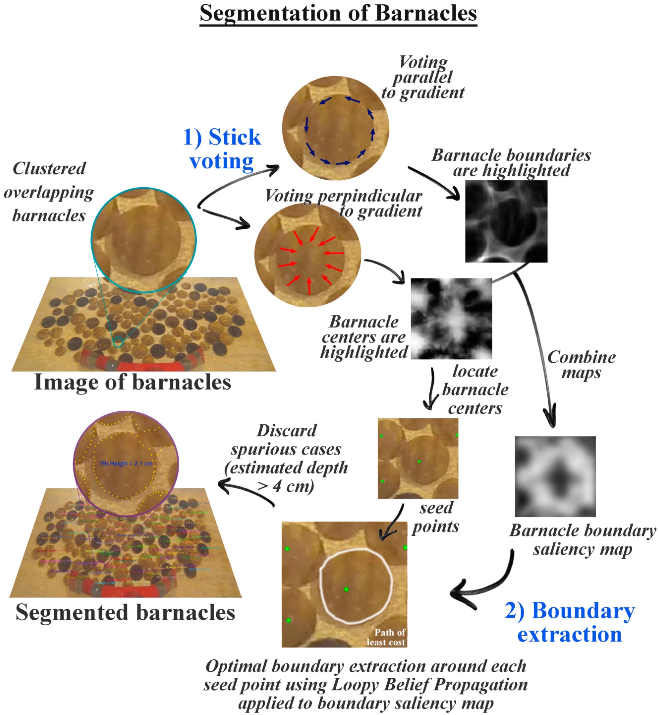
As a preliminary step for identifying the best protocol, each artificial specimen was isolated using an automatic segmentation technique. The segmentation technique is graphically described in Figure 8.
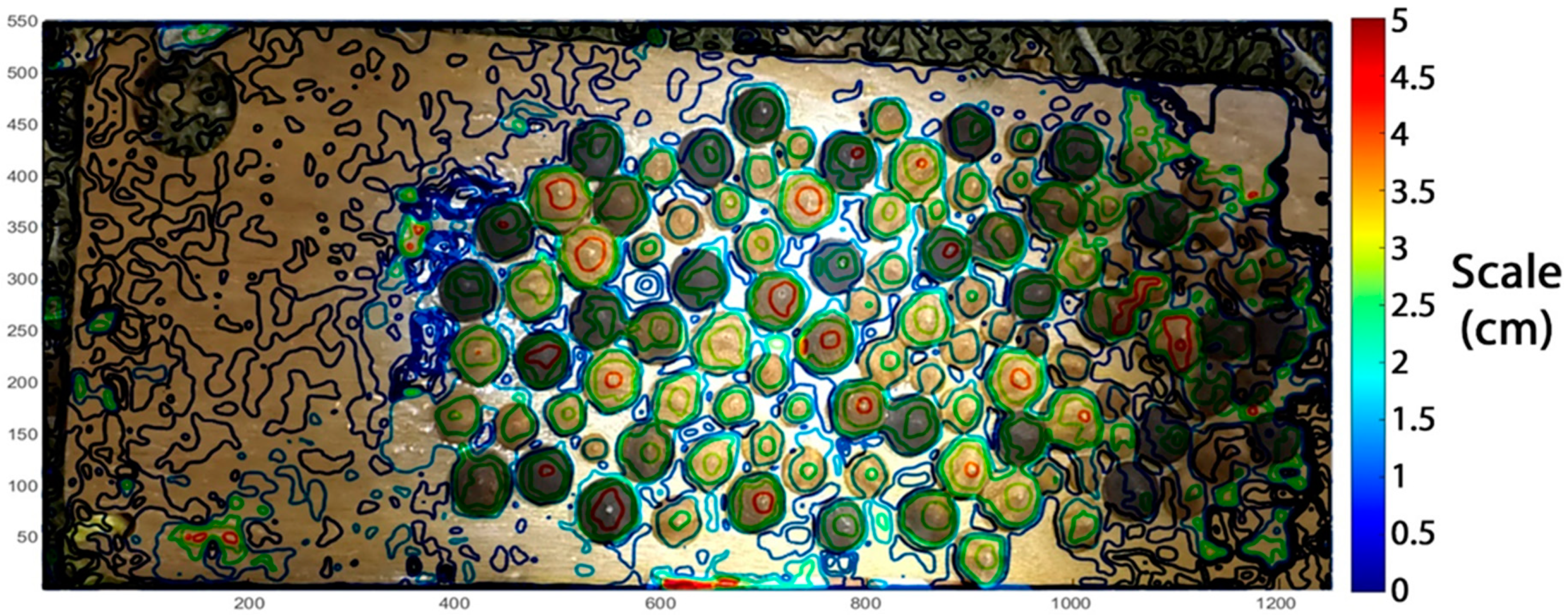
For clustering overlapping specimens, the roughness is defined as the maximum height accessible in each cluster. In the present study, it is always the distance between the peak and the colonized surface (wood plate). To highlight the center of the specimen and the boundaries, stick voting parallel and perpendicular to the gradient is next carried out, followed by optimal boundary extraction around each seed point (specimen centers) using loopy belief propagation [24] applied to the boundary saliency map. Finally, spurious cases are discarded (e.g., too large of a height, for instance more than 40 mm). Key steps are visually presented in Figure 9, Figure 10 and Figure 11. This segmentation is not used for on-site measurements due to the absence of clean surfaces between specimens.

3.2. Configurations of the Tests

To deal with the turbidity, we have changed distances between cameras and the plate by adjusting the length of the jib in clean fresh water with low turbidity. Both flood and spot lighting were selected with camera subject distances of 58 cm, 65 cm, 100 cm, and 120 cm, respectively, with Figure 12 demonstrating how it allows us to cover a wide range of quality of the picture.

3.3. Height Measurement

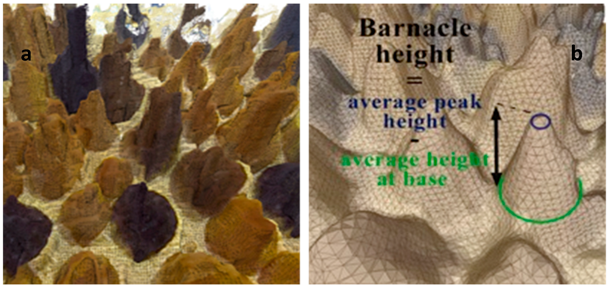
The reference was measured with a dial gauge with an accuracy of 0.1 mm. In Figure 13a, the algorithm provides an estimate of the height of each individual specimen. This was achieved by subtracting the average height values in and around the base of the segmented specimen (represented by the larger circle in Figure 13b) from the maximum height values (represented by the smaller circle in Figure 13b) and by excluding any outlier values (i.e., implausibly large or small heights) that would otherwise skew the measurements if not discarded.

3.4. Indicators of Quality of Measurement

To obtain a distribution of measurements as close as possible to the real one (Figure 3), it was required to detect all the peaks and size them as accurately as possible. Consequently, the probability of detection (PoD) was used as a measure of performance (Equations (1) and (2)), as presented in [25] as an estimate of the peaks and the mean and standard deviation of estimated peaks. The mean and standard deviation were evaluated for estimating the peak sizes first, and the error was deduced from Equation (3) (bias and standard deviation) at the second step.
PoD ( X ) = P ( X a d )
PoD ( X ) N d N t o t
where X is the random variable, the height of artificial specimens; X i and X i ˜ are, respectively, the real and measured values of the specimen; N d and N t o t denote, respectively, the number of detections after boundary extraction and the total number of artificial specimens.
Bias is computed as the mean value of ϵ as
ϵ i X i X i ˜
Receiver operating curves (ROC) have been shown to give a rational and efficient decision tool to compare protocols [26], including for underwater image processing [15]. It plots or fits a curve in the probability of detection (PoD) versus the probability of false alarm (PFA) space, as defined in Equation (4), when the detection threshold ad varies from – to + .
PoD = a d + f S N   ( d ^ )    d   d ^ ; PFA = a d + f N ( η )   d η
where fSN and fN indicate the probability densities of the variables ‘signal + noise’ and ‘noise’ [27], respectively. Here, the noise is the error of measurement and the ‘signal + noise’ is the distribution of measured heights.

3.5. Estimation of Natural Roughness through Fractal Dimension

The natural roughness is more complex than simulated ones. Moreover, the difference of the heights of neighboring peaks governs the drag coefficient [9]. To characterize the roughness of a mature colonization of mussels, the chain of the Biocolmar offshore station was inspected after 2 years. This station is dedicated to the analysis of biofouling of offshore structures with more than 80 coupons. In this paper, we consider the part of the chain to be between 1 m–4 m depth, which was fully colonized by the same thickness of mussels. Three pictures of three parts of this section of the chain were carried out in view to analyze the robustness of the estimates.
First, the ability of the statistical parameters that classically describe the roughness to characterize the fouling was tested. They estimated the dispersion and the shape of the valleys and peaks, computing the average roughness (Equation (5)), the average distance of the peaks to the average roughness (Equation (6)), the standard deviation (Equation (7)), the skewness (Equation (8)), and the kurtosis (Equation (9)) of the roughness.
  R a = 1 M i = 1 M R ( i )
  R m a   = 1 M i = 1 M | R ( i ) R a |
  R s q = 1 M i = 1 M | R ( i ) R a | 2
  R s k = 1   R s q 3 i = 1 M ( R ( i ) R a ) 3
  R k u = 1   R s q 4 i = 1 M ( R ( i ) R a ) 4
Note that parameters   R m a and   R s q do not differentiate between peaks and valleys, and both, with   R s k and   R k u , are sensitive to the distribution and the number of locations.
Next, we will analyze the fractal properties linked to the statistical self-similarity of the data. The fractal dimension (DF) is a further roughness parameter, in addition to the above statistical parameters. Further, the fractal dimension correctly measures the surface roughness itself. For example, two surfaces can have the same skewness or average roughness but different DF (Figure 14).
However, such a link is not necessary for spatial data when both irregularity and the spatial variability of the surfaces are mixed to produce statistical self-similarity. In this case, the similarity can be tested through an infinite range of the scale only on the probability law [28]. The natural fractal of the biofouling surface might be produced from the multi-scaled randomness of the species of the biofouling with different size and at different locations. The fractal dimension DF satisfies the bounds
d < D F < d + 1
where d is the spatial dimension or topologic dimension. When DF = d, the surface is differentiable (smooth), but when it approaches d + 1, the surface is extremely rough. On the other hand, the fractal measure DF is not an integer, and it can be estimated as the limit (known as Box dimension)
  D F = lim h 0 Q ( h ) h
where Q(h) is a spatial statistical quantity (variogram, madogram, periodogram, or number of d-dimensional boxes) and h is a spatial unit. To estimate the fractal dimension of biofouling, 1-D measurements of three trajectories are considered in order to analyze if it is an intrinsic characteristic of a given biofouling, which is mussels in this paper. The most used estimators of DF are proposed using three 1-D trajectories (d = 1) from the biofouling line. Several methods are available for estimating the roughness measure DF and a summary, with their parameters, is provided in Table 1. All methods follow a common procedure that consists of establishing a power law of Q u ( h ) as a function of a small-scale h ≈ 0 (the smallest observed one)
Q u ( h ) h L ( D F )
where the exponent L(.) is a linear application of DF, computed from a linear regression of log ( Q u ( h ) ) on log ( h ) . The cube-count estimate of the fractal dimension consists of counting the number of Euclidian boxes at small scale h, which are required to cover the surface or line R. Then, the DF is estimated as the negative slope of log ( N ( h ) ) versus log ( h ) , where N(h) is the total number of boxes at scale h. This method is sensitive to the amount of area occupied in a grid and the pattern of its distribution [28,29].
The roughness surface is modeled with a rough (non-smooth) spatial stationary random field, typically Gaussian or a transformation of a Gaussian random field with a smooth transformation. Therefore, the geostatistical estimation methods of DF use a linear law between DF and the so called the fractal index 0 < δ < 2. The fractal index characterizes the behavior of some spatial function Q u ( h )   near to the origin, such as the variogram or the madoram of the random field [29,30], or the decay of the spectral density at large frequency.
The variogram and madogram [30] of a random function R(x) are defined by
γ 2 = 1 2 | E [ R ( x + h ) E [ R ( h ) ] | 2
γ 1 = 1 2 | E [ R ( x + h ) E [ R ( h ) ] |  
They satisfy the estimate γ 2 h δ and γ 1 h δ / 2 near the origin (for small h ≈ 0).
Under such circumstances, the fractal dimension quantifies the curvature of the variogram or madogram near the origin, which characterizes the roughness of the surface.
The periodogram method uses the behavior of the spectral density at infinity. The periodogram is an estimate of the spectral density, defined by
S ( p ) = 2 0 c ( x ) cos ( p x ) d x  
where the spatial correlation c is approximated by the empirical correlation using the spatial mean of all contribution distant with a given lag h. Further, we use the discrete Fourier transform (DFT) to compute the periodogram Q(h) as an estimate of the spectral density S. Therefore, by using the decay of the spectral density that decreases at infinity, it is similar to the bound O ( p δ 1 ) [31]. Here, DF is estimated from a regression fit of log ( Q ( h ) ) versus log ( h ) .   Table 1 summarizes the methods considered and compared for estimating the fractal dimension of the rough curve (of the graph). This measure of roughness is estimated only from the data and independently of the covariance model of the random field. Once the fractal dimension is estimated, a spatial model can be chosen with adequate fractal index from the estimated fractal dimension to quantify the hydrodynamic forces.
Finally, these estimates are subjected to a statistical error. To obtain the confidence interval for various DF estimates, we use the parametric bootstrap method, as proposed by [32]. The method starts with an appropriate model of the covariance function to well fit the spatial data. The powered exponential correlation is largely used in the literature and is defined by:
c ( h ) = exp ( | h c | δ )
It is an appropriate model since it is a valid covariance for all values of the fractal index δ in (0, 2). Further, the model is only smooth when δ = 2.
Fractal based detection has been applied successfully to build infrastructure systems before [33], including renewable energy device platforms [34], and the non-detection aspects are also known [35,36]. This approach further establishes this measure as a core feature for biofouling effects.

4. Results in Laboratory and on Site

4.1. Results from Measurements for Each Protocol in Laboratory

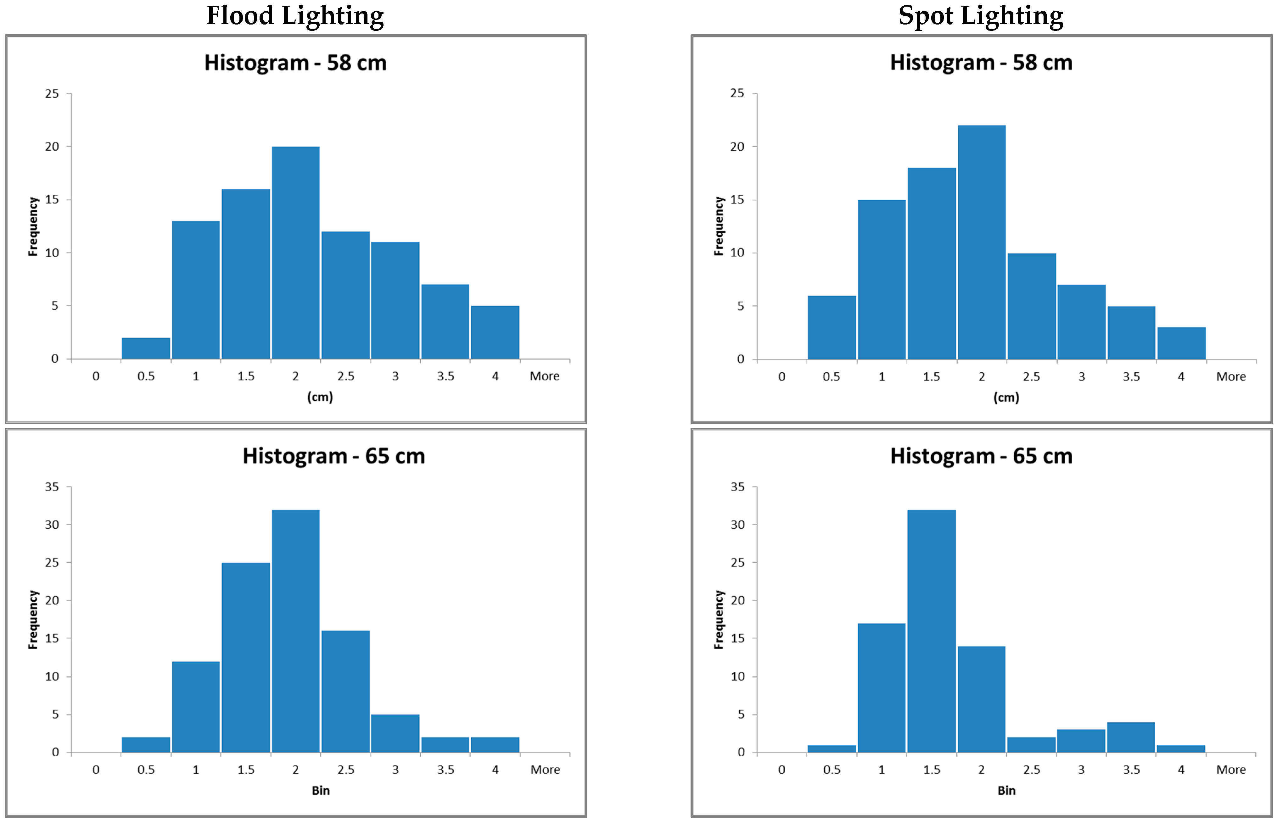
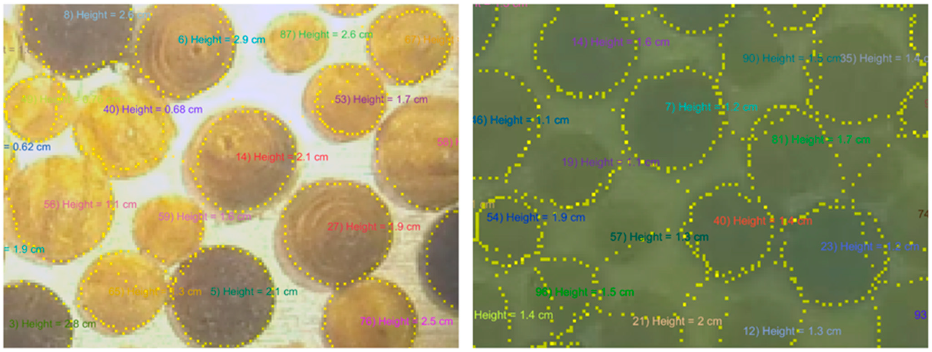
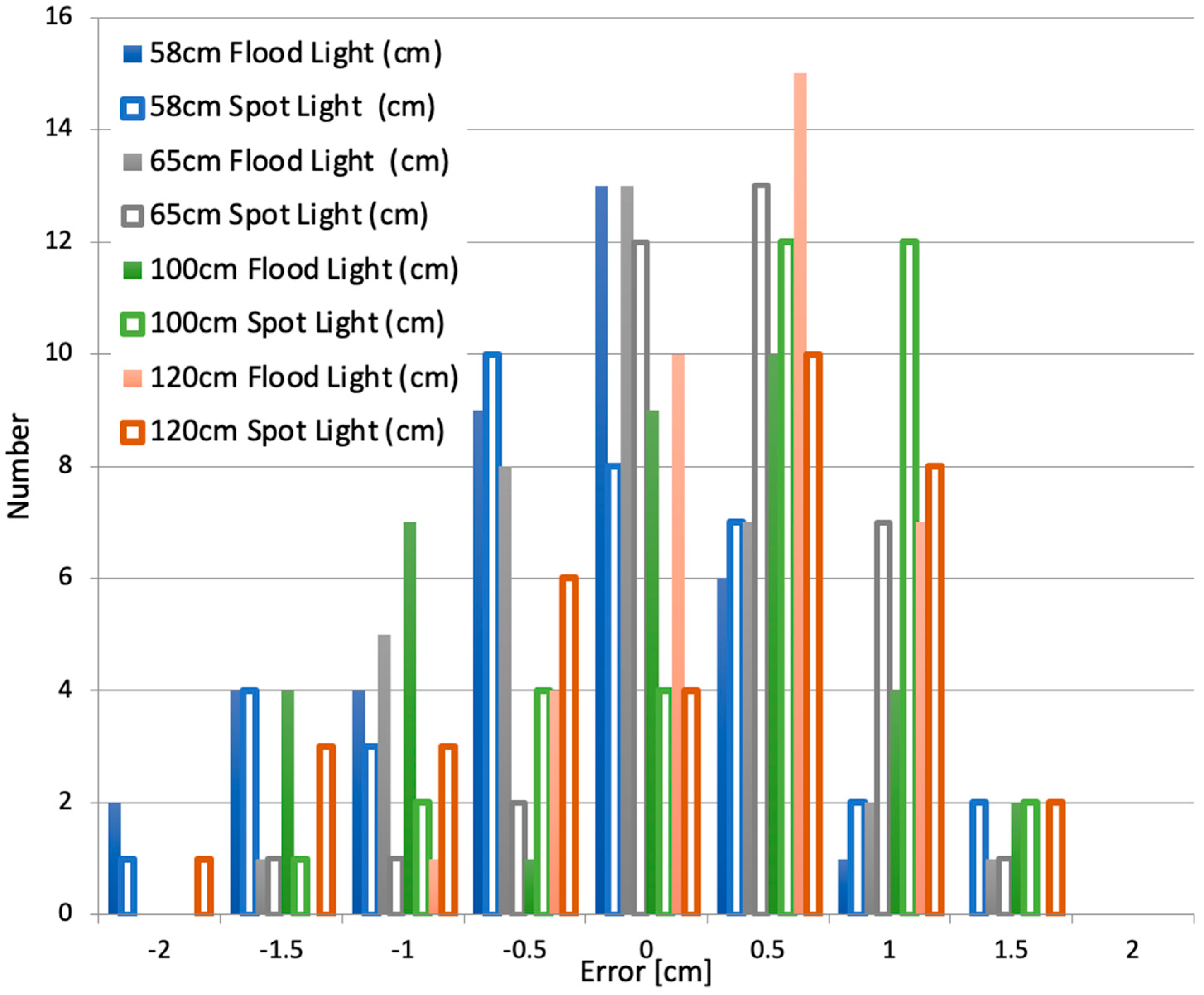
The histograms of the measured heights are plotted for various device set-ups in terms of lighting and distance (Figure 15). Depending on the distance to the target, flood, or spot lights, this can lead to more or less favorable conditions. For instance, Figure 16 illustrates that the spot light gives a high contrast picture for a small distance (58 cm) but a small area of the clear image, whereas the contrast is low, but the area is large when the distance increases to 120 cm.
The shape of the distribution is significantly different from the original Figure 3, with a clear asymmetry and a single mode of the distribution except for 120 cm and 65 cm flood lighting conditions. For these two setups a second mode is captured around 3 cm, whereas for the actual figure it is around 2 cm.
The asymmetry can be assessed by computing the skewness (Table 2).
Results show that, in contrary to the real distribution, the skewness of measured distribution is significant (between 0.3–1.2).

4.2. Evaluation of the Indicators in Laboratory

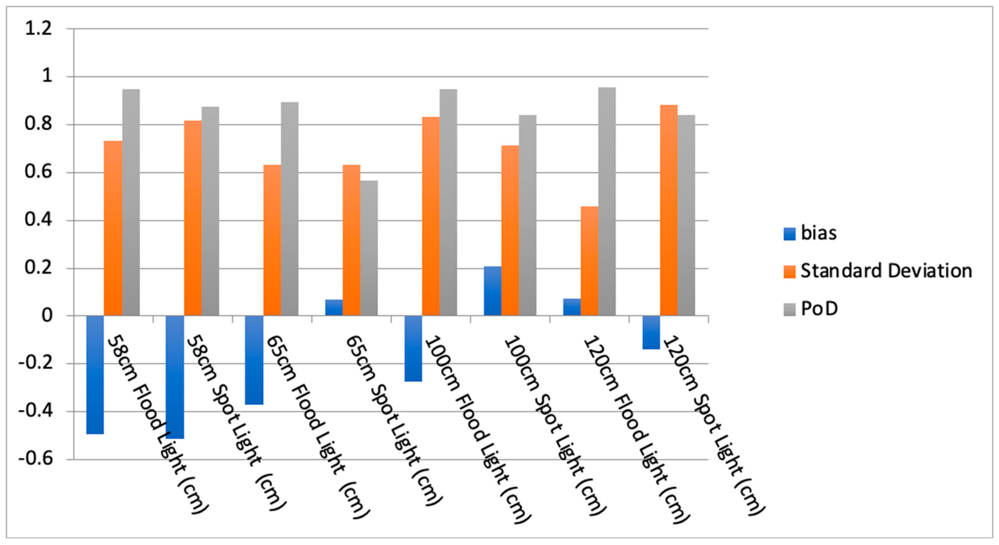
With selected indicators evaluated, the probability of detection (PoD) is computed from the data base of 95 measurements and is plotted in Figure 17. The PoD varies from 0.55 (65 cm, spot light) to 0.95 (58 cm; 100 cm; 120 cm flood light), indicating that the flood light provides better conditions when limiting the number of missed detections.
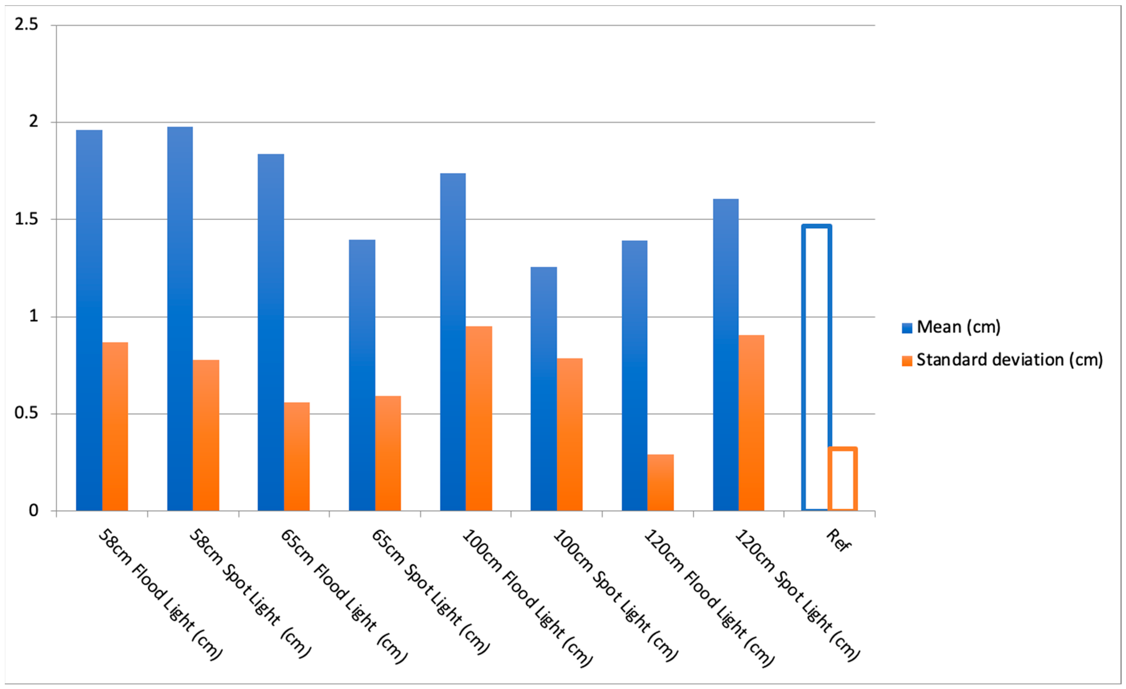
The two first moments (mean, standard deviation) are estimated next in Figure 18 and are compared to the reference (real value). The protocol 120 cm-flood light is one of the best, with a 58 cm-spotlight being the worst, despite performing well in terms of PoD (85%). This criterion is thus observed to be complementary to PoD estimates. Table 3 gives the relative errors of the mean (5–35%) and the standard deviation (10–200%). According to this criterion, the best protocol is the 120 cm-flood light (in bold in Table 3), which was already selected according to the PoD criterion, corresponding to a 5% error in mean and a 10% error in standard deviation (10%).
Finally, the distribution of error was assessed. The mean value (bias) and the standard deviation of this distribution are reported in Figure 19. The bias was observed to range from −0.5 to +0.2 cm, and the standard deviation stays in the range 0.5–0.95. Once again, the protocol 120 cm-spotlight gave the best results with a bias of 0.05 and a standard deviation of 0.5. It is noteworthy to highlight that the 65 cm-spotlight leads to a very low error (bias of 0.05 and standard deviation of 0.65), but the PoD was very low for this protocol.
This last estimate shows a good assessment for the 120 cm-flood light, with 5 and 10% of error, respectively, of the mean and standard deviation. The bias has been shown to reach −0.5 cm if optimal conditions are not gathered.
The effect on loading through the computation of drag coefficients is analyzed next. Two types of structures are considered for which the loading can be computed through Morison’s equation. The first structure is a mooring line with a rope of an equivalent diameter of 30 cm, and the second one is structural members of a jacket structure with an equivalent diameter of 1.2 m colonized with marine growth of a roughness of 2 cm. The global effect of marine growth has been studied and quantified [8,9,10]. These studies highlight that roughness affects steady flow drag coefficient CDS through the relative roughness e = k/De, where k is the roughness and De is the diameter. With the above diameters of 0.3 and 1.2m, e takes values of 0.07 and 0.018, respectively, and according to API [11] CDS, takes values of 1.1 and 1.07, respectively. An error of −0.5 cm leads, respectively, to errors of e of −0.017 and −0.004, which produces a negligible change of −0.005 (0.5%) and −0.01 (1%) on CDS. A lower bias (0.05 for 120 cm-flood light) allows for a very good accuracy for an assessment of the distribution and the fractal dimension.

4.3. ROC Curves for Detection Assessment in Laboratory

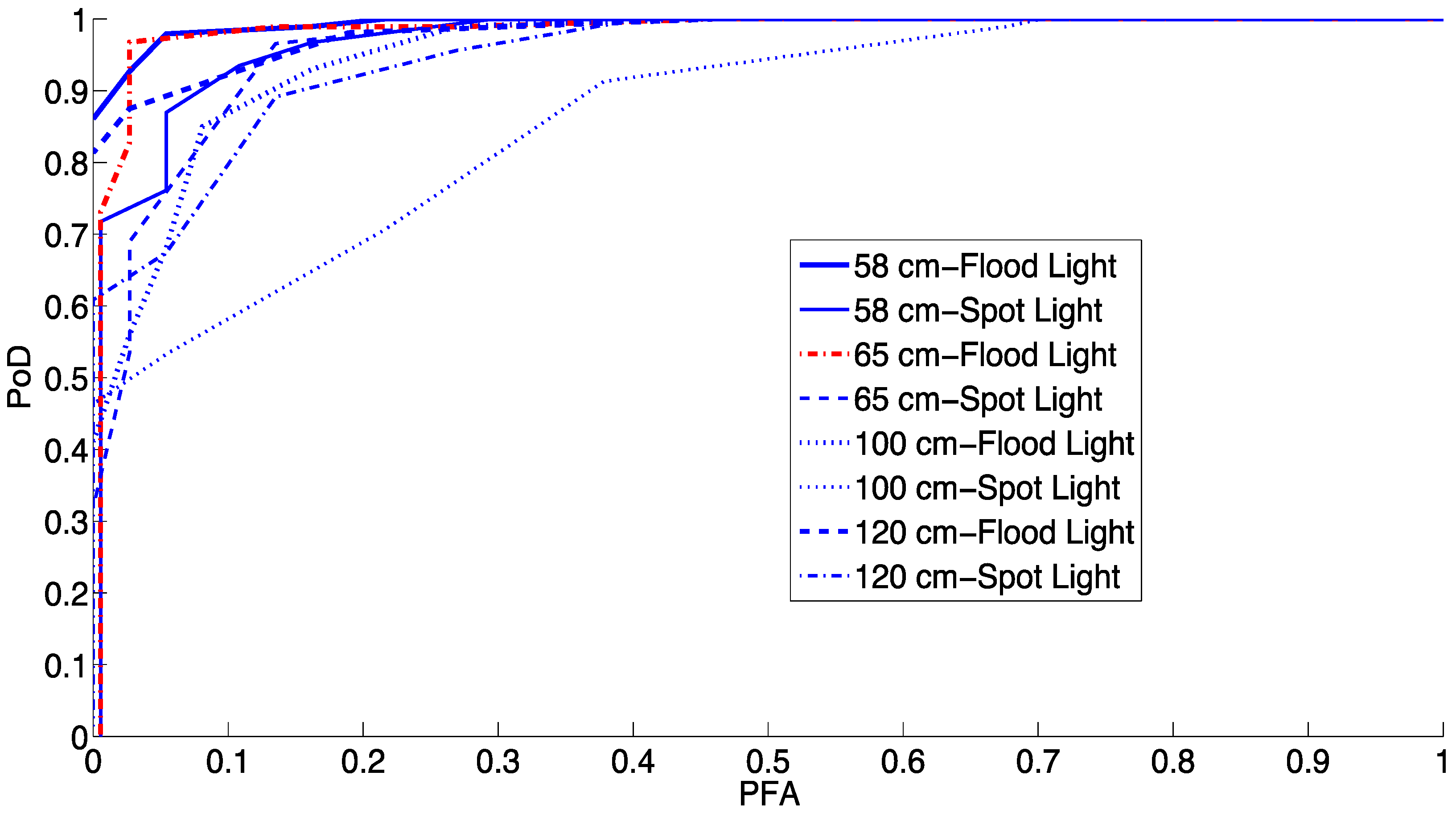
Figure 19 plots the distributions of errors for each protocol. For discrete values, we estimated the probabilities by computing statistical frequencies [37]. ROC curves are plotted in Figure 20. Protocols with spot light are among the worst ones.
Protocol of the 100cm-spotlight distinguishes itself from others with the bar ROC curve. The best one, plotted in a red dashed line, corresponds to the 65 cm-flood light. This quality can be quantified by δ, the distance between the point of coordinates (0,1) (absolute best performance point) and the ROC curve [38], reported in Table 4; the point on the ROC is called the best performance point. It is shown that δ is the smallest for the 65cm-flood light (0.04) and 58 cm-flood light (0.06) protocols. The point on the ROC curve corresponding to this smallest value allows computing of the detection threshold ad defined in (4); this threshold is an optimal value in the sense that it minimizes the PFA while maximizing the PoD. Its values are reported in Table 4, and, for the smallest δ, there are 0.5 cm (protocol 58 cm-flood light) and 0.75 cm (65 cm-flood light). It is important to note here that 0.7 cm was the smallest height of artificial roughness, and only 0.75 cm has a sense, marked in bold in the table. Note that ad distance is similar for performances that change significantly; this is due to the definition of ad that is related to the angle α between the line between (0;1) and coordinates of the best performance point and the y-axis. More details can be found in [38].

4.4. 2D-Fractal Dimension Assessment on Site

The protocol selected in the previous section (65 cm-flood light) was selected for assessing the roughness on site and the photos in Figure 3. The corresponding profile of roughness is plotted in Figure 21.
The two first statistical moments of these trajectories and the coefficient of variation are computed next, as reported in Table 5.
These statistics show that there are some similarities (10% of discrepancy in mean) but also some differences (30% of discrepancy in standard deviation). When looking at the trajectories on Figure 22, it is observed that the global shape due to the spatial arrangement of mussels should be assessed.
The statistical parameters related to roughness estimates are computed subsequently by estimating the dispersion and the shape of the valleys and peaks (Table 6).
The discrepancies are significant (15% to 150%) depending on the parameter. The fractal dimension is then assessed and reported in Table 7.
All estimates of the fractal dimensions show a considerable roughness for the profiles (DF > 1). Further, except estimates given by the periodogram method, estimates give some isotropy of the roughness (isotropic spatial random field with the same regularity). Furthermore, the absence of relationship between madogram and variogram estimates can suggest modeling of the curves R1, R2, and R3 with non-Gaussian random fields (for example a log-normal random field can be more adequate) because in the case of the Gaussian random surface, the madogram satisfies γ 1 = γ 2 [30]. We chose an estimate of the fractal dimension that has a tick confidence interval of DF.
Figure 22 depicts the boxplots of the fractal dimension estimates from simulated data using the powered exponential model. It shows that the method of the periodogram gives more dispersed estimates than the other methods, while the estimate from the method of the variogram is less dispersed. Further, the madogram estimate can be seen as more efficient than the cube-count estimator and the periodogram estimator.
Under the assumption of isotropy between the two directions of the surface and by considering the average of the fractal dimension of the curves from the variogram estimates (Table 7), we approximate the fractal dimension of the surface roughness by DF ≈ 9/4.

5. Discussion and Conclusions

Assessment of roughness from on-site inspection is required to improve the updating of hydrodynamic forces after inspection, to better predict the service lifetime, and to optimize the operation and maintenance planning. This geometrical parameter is shown to have a significant impact on the drag coefficients. It was first mentioned in aerodynamics studies [39,40,41], and it was found that the roughness density plays a critical role in the mean forces and pressures. Fuss [42] showed that, in addition to the maximal and mean surface roughness, the surface skewness is a further roughness parameter that affects the critical Reynolds number and the lift/drag coefficients. With offshore renewable energy on the rise, this is an important topic to focus on.
With the rise of the importance of drones, image processing is bound to play an important role in this regard through inspection driven maintenance of lifetime performance needs of offshore wind turbines. This paper investigates two key control parameters of such inspections, through stereo-imaging, to obtain information about their roughness and establish their applicability through comparative performance under controlled and semi-controlled conditions. The 120 cm-flood light protocol for testing was shown to be a good candidate, with the highest PoD, lowest errors on the mean and standard deviation, lowest bias and standard deviation of error, and best for establishing the modes of distribution appropriately. This protocol, however, performed poorly for skewness. Consequently, a detailed study with ROC curves was carried out to understand if a more robust approach of selecting testing protocols existed, since a highly sensitive but less robust method may not be the best to use. This approach elicited a 65cm-flood light protocol as the appropriate method for a range of performance conditions, and it was robust against environmental variations, which are often important criteria for field implementation. Both of these comparative protocols with varied performance advantages lead to a detection threshold of 7.5 mm.
Subsequent site implementation to estimate mussel roughness indicated that the complexity the of natural shapes requires more sophisticated methods for such assessments than what might be apparent from controlled tests, which are often carried out in various laboratories. The 2-D fractal dimension was observed to be a good feature for such estimation, especially when computed via madogram. Similar and long-term studies around spatial and temporal growth of various species (e.g., oysters, barnacles) have the potential to calibrate such roughness against fractal dimensions in the form of comprehensive experimental mapping.
To choose a method or a feature for inspection implementation, it is typically guided by risk-based inspection methodology [25,27,43], and there will remain the question of a calibration gap between real-world imagery and synthetic data. However, ‘trust’ on such virtual data [44] can be improved through choosing robust features such as the fractal dimension presented here. Machine learning and deep learning are popular, but such methods tend to not capture realistic details in a simulated environment and can underperform in real environments. Consequently, damage-assessment algorithms trained with synthetic data may not generalize well for real-world examples, including the semantics that influence such detection processes [45]. Therefore, it is prudent to collect some degree of ’real’ data in order to validate statistical learning models, especially in the context of calibrating features such as the fractal dimensions [46]. This paper is timely since the results are particularly relevant for floating wind turbines, a sector that is seeing a surge at the moment and is expected to evolve rapidly in an interdisciplinary manner, with the requirements of aspects such as biofouling entering at earlier TRLs. Such biofouling will also impact the lifetime fatigue of the turbine base, and the possibility of reuse of the site following the completion of the lifetime of a turbine will also be a function of such growths, distributions, and rates.
The choice of more than one statistical marker highlights the requirement to focus on a set of admissible markers, rather than trying to establish the best marker. The advantage of this approach is that, while they outperform each other in terms of various metrics based on a specific environment, they will be robust against changes and provide an overall comparable performance, as evidenced by their proximity in the ROC space.
The work also creates a future possibility of investigating the interaction of multiple species, such as barnacles and mussels, with ecological compatibility required to be established in terms of their growth rates, predator presence, and related hydrodynamic impacts. Field experiments in the seasonal site of the northern gulf of California [47] experimentally demonstrated how the mussel–barnacle community is close [48] and influence each-other, as has been indicated by other works [49,50]. The competition from mussels comes at lower shore levels to barnacles [51] where rock space becomes less for barnacle settlement. Barnacles on living mussel shells grow faster than empty shells, but the presence of barnacles seems to have little effect on mussel growth [52]. While there is a hierarchy of species, as is expected in an ecology [53], their close interaction [54,55] remains a well-documented aspect. This ecological aspect is another area where continued work is needed.
It is difficult to compare the quantitative results presented in this paper with other studies, as the proposed methodology and the detection method is new. However, relevant works on varied, controlled lighting conditions, created in the laboratory [15] or synthetically [45], indicate that the ROC space, region of operation, and best performance points established from image processing [17,56,57,58] are similar to what has been obtained in this paper. Fractal estimates on corrosion images [59] indicate how this feature can be an indicator of gradual degradation. Soil–water interaction and pore solid distributions have extensively considered fractal estimates as well [60,61,62,63,64,65]. While a quantitative estimate comparison is not meaningful here, the consistency of the fractal estimates with gradual and consistent changes and their monotonicity of their relationship indicate how the current work can be influential in developing and calibrating the markers of such changes from image processing around hard biofouling. This characterization subsequently has the impact of influencing scaled testing in ocean wave basin tests at lower TRLs and is relevant for offshore renewable energy.
The concept of ’digital twin’ is attracting growing interest and appears to be a prominent research direction for offshore marine structures [66,67]. A close similarity between a virtual and physical structure will allow for better monitoring and data analysis of such systems, leading to early detection of features of interest [68] and lower downtime and allow for improved decisions on future remedial actions through scenario assessment [69]. It is also expected that this paper will be relevant for offshore experimental sites around biofouling [70] and marine heritage [71].

Author Contributions

Conceptualization, F.S.; methodology, F.S., B.G., M.O. (Michael O’Byrne), V.P., M.O. (Mestapha Oumouni), T.S. and M.R.; software, M.O. (Michael O’Byrne), M.O. (Mestapha Oumouni), M.R.; validation, M.O. (Michael O’Byrne), B.G. and M.O.; formal analysis, M.O. (Michael O’Byrne), M.O., T.S., M.R.; investigation, F.S., V.P., M.O., T.S., M.R.; resources, F.S., B.G. and V.P.; data curation, F.S.; writing—original draft preparation, F.S., M.O. (Mestapha Oumouni), T.S. and M.R.; writing—review and editing, M.O. (Michael O’Byrne), B.G. and V.P.; visualization, M.O. (Michael O’Byrne) and M.O. (Mestapha Oumouni); supervision, F.S., B.G. and V.P.; project administration, F.S., B.G. and V.P.; funding acquisition, F.S., B.G. and V.P. All authors have read and agreed to the published version of the manuscript.

Funding

Authors are grateful to Hamed Ameryoun (IXEAD, Capacités SAS company, Université de Nantes, France) and Christian Berhault (senior Consultant) for their help in LEHERO-MG and ABIOP projects. This work was carried out within the project LEHERO-MG (Load Effect of HEterogeneous ROughness of Marine Growth) granted by WEAMEC, West Atlantic Marine Energy Community with the support of Région Pays de la Loire and in partnership with Naval Energies (Françoise Dubois). Tests were carried out within the french national project ABIOP (2017–2018) in collaboration with “France Energies Marines” (Nolwenn Quillien and Guillaume Damblans) and has benefited from state aid managed by the French National Research Agency (ANR-10 IEED-0006-21). V.P would like to acknowledge ERA-NET Cofund MarTERA FLEXAQUA project PBA/BIO/18/02, The Marine Institute, Ireland, SFI MaREI Centre (12/RC/2302_2) and The Energy Institute, UCD for this work. B.G. would like to acknowledge SFI Connect centre for this work.

Institutional Review Board Statement

Not applicable.

Informed Consent Statement

Not applicable.

Data Availability Statement

Data is available from the authors on request. Additionally, for a range of data, the authors should consider https://ultir.github.io/ (accessed on 17 November 2021).

Conflicts of Interest

The authors declare no conflict of interest.

References

  1. Heaf, N.J. The Effect of Marine Growth on the Performance Of Fixed Offshore Platforms in the North Sea. In Proceedings of the Offshore Technology Conference, Houston, TX, USA, 30 April–3 May 1979; p. 14. [Google Scholar] [CrossRef]
  2. Jusoh, I.; Wolfram, J. Effects of marine growth and hydrodynamic loading on offshore structures. J. Mek. 1996, 1, 77–98. [Google Scholar]
  3. Picken, G.B. Review of Marine Fouling Organisms in the North Sea on Offshore Structures. Discussion Forum and Exhibition on Offshore Engineering with Elastomers; Plastics and Rubber Instute: UK, London, 1985; Volume 5, pp. 5.1–5.10. [Google Scholar]
  4. Boukinda, M.L.; Schoefs, F.; Quiniou, R.V.; Birades, M. Marine growth colonization process in guinea gulf: Data analysis. J. Offshore Mech. Arct. Eng. 2007, 129, 97–106. [Google Scholar] [CrossRef]
  5. Ameryoun, H. Probabilistic Modeling of Wave Actions on Jacket Type Offshore Wind Turbines in Presence of Marine Growth. Ph.D. Thesis, Université de Nantes Faculté des Sciences et des Techniques, Nantes, France, 2015. [Google Scholar]
  6. Theophanatos, A. Marine Growth and Hydrodynamic Loading of Offshore Structures. Ph.D. Thesis, University of Strathclyde, Glasgow, UK, 1988. [Google Scholar]
  7. Zdravkovich, M.M. Flow Around Circular Cylinders, 1st ed.; Oxford University Press: Oxford, UK, 2002; Volume 2. [Google Scholar]
  8. Schoefs, F.; Boukinda, M.L. Sensitivity Approach for Modelling Stochastic Field of Keulegan Carpenter and Reynolds Number Through a Matrix Response Surface. J. Offshore Mech. Arct. Eng. 2010, 132, 1–7. [Google Scholar] [CrossRef] [Green Version]
  9. Ameryoun, H.; Schoefs, F.; Barillé, L.; Thomas, Y. Stochastic modeling of forces on jacket-type offshore structures colonized by marine growth. J. Mar. Sci. Eng. 2019, 7, 158. [Google Scholar] [CrossRef] [Green Version]
  10. Schoefs, F. Sensitivity approach for modelling the environmental loading of marine structures through a matrix response surface. Reliab. Eng. Syst. Saf. 2008, 93, 1004–1017. [Google Scholar] [CrossRef] [Green Version]
  11. API-RP-2A WSD. Recommended Practice for Planning, Designing and Constructing Fixed Offshore Platforms-Working Stress Design; American Petroleum Institute: Washington, DC, USA, 2005. [Google Scholar]
  12. DNV. Recommended Practice DNV-RP-C205. Environmental Conditions and eEvironmental Loads; Det Norske Veritas: Hovik, Norway, 2017. [Google Scholar]
  13. Bakhtiari, A.; Schoefs, F.; Ameryoun, H. Unified Approach for Estimating of the drag Coefficient in Offshore Structures in Presence of Bio-Colonization. In Proceedings of the 37th International Conference on Offshore Mechanics and Arctic Engineering (ASME 2018), Madrid, Spain, 30 December 2018; p. 7. [Google Scholar]
  14. Bakhtiari, A.; Schoefs, F.; Ameryoun, H. A review of the biofouling parameters influencing the drag force coefficient of offshore structures. In Proceedings of the 3rd International Conference on Renewable Energies Offshore (RENEW 2018), Lisbon, Portugal, 8–10 October 2018; p. 8. [Google Scholar]
  15. O’Byrne, M.; Schoefs, F.; Pakrashi, V.; Ghosh, B. An underwater lighting and turbidity image repository for analysing the performance of image based non-destructive techniques. Struct. Infrastruct. Eng. 2018, 14, 104–123. [Google Scholar] [CrossRef] [Green Version]
  16. OByrne, M.; Ghosh, B.; Schoefs, F.; Pakrashi, V. Image-Based Damage Assessment for Underwater Inspections, 1st ed.; CRC Press: Boca Raton, FL, USA, 2018; ISBN-10: 1138031860. [Google Scholar]
  17. OByrne, M.; Schoefs, F.; Pakrashi, V.; Ghosh, B. A Stereo-Matching Technique for Recovering 3D Information from Underwater Inspection Imagery. Comput. Aided Civ. Infrastruct. Eng. 2018, 33, 193–208. [Google Scholar] [CrossRef]
  18. Decurey, B.; Schoefs, F.; Barillé, A.L.; Soulard, T. Model of Bio-Colonisation on Mooring Lines: Updating Strategy based on a Static Qualifying Sea State for Floating Wind Turbine. J. Mar. Sci. Eng. 2020, 8, 108. [Google Scholar] [CrossRef] [Green Version]
  19. Quirk, L.; Matos, J.; Murphy, J.; Pakrashi, V. Visual Inspection and Bridge Management. J. Struct. Infrastruct. Eng. 2018, 14, 320–332. [Google Scholar] [CrossRef]
  20. O’Donnell, D.; Murphy, J.; Pakrashi, V. Comparison of Response Amplitude Operator Curve Generation Methods for Scaled Floating Renewable Energy Platforms in Ocean Wave Basin. ASME Lett. Dyn. Syst. Control 2021, 1, 021012. [Google Scholar] [CrossRef]
  21. ODonnell, D.; Murphy, J.; Pakrashi, V. Damage Monitoring of a Catenary Moored Spar Platform for Renewable Energy Devices. Energies 2020, 13, 3631. [Google Scholar] [CrossRef]
  22. LEHERO-MG. Load Effect of Heterogeneous Roughness of Marine Growth–2017–2020. Research Project Founded by WEst Atlantic Marine Energy Community and Leaded by Université de Nantes (Pr. F. Schoefs). Available online: https://www.weamec.fr/en/projects/lehero-mg/ (accessed on 17 November 2021).
  23. Bakhtiari, A.; Schoefs, F.; Berhault, C.; Ameryoun, H. Evaluation of marine growth parameters effects on offshore structures loading. In Proceedings of the 54th ESReDA Seminar on Risk, Reliability and Safety of Energy Systems in Coastal and Marine Environments Nantes, Nantes, France, 25–26 April 2018. [Google Scholar]
  24. OByrne, M.; Schoefs, F.; Ghosh, B.; Pakrashi, V. Evaluation of camera calibration techniques for quantifying deterioration. In Proceedings of the Civil Engineering Research in Ireland 2016 (CERI2016), National University of Ireland, Galway, Ireland, 29–30 August 2016. [Google Scholar]
  25. Rouhan, A.; Schoefs, F. Probabilistic modeling of inspection results for offshore structures. Struct. Saf. 2003, 25, 379–399. [Google Scholar] [CrossRef] [Green Version]
  26. Pakrashi, V.; Schoefs, F.; Memet, J.B.; OConnor, A. ROC Dependent Event Isolation Method for Image Processing Based Assessment of Corroded Harbour Structures. J. Struct. Infrastruct. Eng. 2010, 6, 365–378. [Google Scholar] [CrossRef] [Green Version]
  27. Schoefs, F. Modeling Inspection Uncertainties for In-site Condition Assessment using NDT tool. In Maintenance and Safety of Aging Infrastructure; Frangopol, D., Tsompanakis, Y., Eds.; Structures and Infrastructures Book Series; CRC Press: Boca Raton, FL, USA, 2014; Volume 10, Chapter 19; pp. 573–619. [Google Scholar]
  28. Mandelbrot, B.B. Fractals: Forms, Chance and Dimension; Book Freeman: San Francisco, CA, USA, 1977. [Google Scholar]
  29. Adler, R.J. The Geometry of Random Fields. Camb. Philos. Soc. 1981, 91, 57–74. [Google Scholar]
  30. Allard, D.; Chilès, J.-P.; Delfiner, P. Geostatistics: Modeling Spatial Uncertainty; Wiley: New York, NY, USA, 2013; Volume 45, pp. 377–380. [Google Scholar]
  31. Stein, M.L. Interpolation of Spatial Data: Some Theory for Kriging. In Springer Series in Statistics; Springer: New York, NY, USA, 1999. [Google Scholar]
  32. Davies, S.; Hall, P. Fractal analysis of surface roughness by using spatial data. J. R. Stat. Soc. Stat. Methodol. 1999, 61, 3–37. [Google Scholar] [CrossRef]
  33. Pakrashi, V.; Kelly, J.; Harkin, J.; Farrell, A. Hurst Exponent Footprints from Activities on a Large Structural System. Physica A 2013, 392, 1803–1817. [Google Scholar] [CrossRef]
  34. Pakrashi, V.; OShea, R.; Jaksic, V.; Murphy, J. The Hurst Exponent as an Indicator of the Behaviour of a Model Monopile in an Ocean Wave Testing Basin. J. Phys. 2015, 628, 012057-1-8. [Google Scholar] [CrossRef]
  35. Pakrashi, V.; Basu, B.; OConnor, A. Non-Detection, False Alarm and Calibration Insensitivity in Kurtosis and Pseudofractal Based Singularity Detection. ASCE J. Aerosp. Eng. 2009, 22, 466–470. [Google Scholar] [CrossRef] [Green Version]
  36. Pakrashi, V.; OConnor, A.; Basu, B. A Comparative Analysis of Structural Damage Detection Techniques by Wavelet, Kurtosis and Pseudofractal Methods. Struct. Eng. Mech. 2009, 32, 489–500. [Google Scholar] [CrossRef] [Green Version]
  37. Schoefs, F.; Abraham, O.; Popovics, J. Quantitative evaluation of NDT method performance: Application example based on contactless impact echo measurements for void detection in tendon duct. Constr. Build. Mater. 2012, 37, 885–892. [Google Scholar] [CrossRef] [Green Version]
  38. Schoefs, F.; Boéro, J.; Clément, A.; Capra, B. The αδ method for modelling expert Judgment and combination of NDT tools in RBI context: Application to Marine Structures. Struct. Infrastruct. Eng. 2012, 8, 531–543. [Google Scholar] [CrossRef] [Green Version]
  39. Achenbach, E.; Heinecke, E. On vortex shedding from smooth and rough cylinders in the range of Reynolds numbers 6.103 to 5.106. J. Fluid Mech. 1981, 109, 239–251. [Google Scholar] [CrossRef]
  40. Ribeiro, J.D. Effects of surface roughness on the two-dimensional flow past circular cylinders I: Mean forces and pressures. J. Wind. Eng. Ind. Aerodyn. 1991, 37, 299–309. [Google Scholar] [CrossRef]
  41. Ribeiro, J.D. Effects of surface roughness on the two-dimensional flow past circular cylinders II: Fluctuating forces and pressures. J. Wind. Eng. Ind. Aerodyn. 1991, 37, 311–326. [Google Scholar] [CrossRef]
  42. Fuss, F.K. The effect of surface skewness on the super/postcritical coefficient of drag of roughened cylinders. Procedia Eng. 2011, 13, 284–289. [Google Scholar] [CrossRef] [Green Version]
  43. Faber, M.H. Risk-Based Inspection: The Framework. Struct. Eng. Int. 2002, 12, 186–195. [Google Scholar] [CrossRef]
  44. O’Byrne, M.; Ghosh, B.; Schoefs, F.; Pakrashi, V. Applications of Virtual Data in Subsea Inspections. J. Mar. Sci. Eng. 2020, 8, 328. [Google Scholar] [CrossRef]
  45. O’Byrne, M.; Pakrashi, V.; Schoefs, F.; Ghosh, B. Semantic Segmentation of Underwater Imagery Using Deep Networks Trained on Synthetic Imagery. J. Mar. Sci. Eng. 2018, 6, 93. [Google Scholar] [CrossRef] [Green Version]
  46. Tricot, C. Two definitions of fractional dimension. Math. Proc. Camb. Philos. Soc. 1982, 91, 57–74. [Google Scholar] [CrossRef]
  47. Lively, C.M.; Raimondi, P.T. Desiccation, predation, and mussel-barnacle interactions in the northern Gulf of California. Oecologia 1987, 74, 304–309. [Google Scholar] [CrossRef]
  48. Bell, C.M. The Epibiotic Relationship between Mussels and Barnacles. Ph.D. Thesis, Rhodes University, Grahamstown, South Africa, 2013. [Google Scholar]
  49. Menge, B.A.; Hacker, S.D.; Freidenburg, T.; Lubchenco, J.; Craig, R.; Rilov, G.; Noble, M.; Richmond, E. Potential impact of climate-related changes is buffered by differential responses to recruitment and interactions. Ecol. Monogr. 2011, 81, 493–509. [Google Scholar] [CrossRef] [Green Version]
  50. Kawai, T.; Tokeshi, M. Asymmetric coexistence: Bidirectional abiotic and biotic effects between goose barnacles and mussels. J. Anim. Ecol. 2006, 75, 928–941. [Google Scholar] [CrossRef] [Green Version]
  51. Luckens, P.A. Competition and intertidal zonation of barnacles at Leigh, New Zealand. N. Z. J. Mar. Freshw. Res. 1975, 9, 379–394. [Google Scholar] [CrossRef]
  52. Laihonen, P.; Furman, E.R. The site of settlement indicates commensalism between bluemussel and its epibiont. Oecologia 1986, 71, 38–40. [Google Scholar] [CrossRef]
  53. Yakovis, E.; Artemieva, A. Cockles, barnacles and ascidians compose a subtidal facilitation cascade with multiple hierarchical levels of foundation species. Sci. Rep. 2017, 7, 1–11. [Google Scholar]
  54. Dungan, M.L. Three-Way Interactions: Barnacles, Limpets, and Algae in a Sonoran Desert Rocky Intertidal Zone. Am. Nat. 1986, 127, 292–316. [Google Scholar] [CrossRef]
  55. Silliman, B.R.; McCoy, M.; Trussell, G.C.; Crain, C.M.; Ewanchuk, P.J.; Bertness, M.D. Non-Linear Interactions between Consumers and Flow Determine the Probability of Plant Community Dominance on Maine Rocky Shores. PLoS ONE 2013, 8, e67625. [Google Scholar]
  56. O’Byrne, M.; Schoefs, F.; Pakrashi, V.; Ghosh, B. A Regionally Enhanced Multi-Phase Segmentation Technique for Damaged Surfaces. Comput. Aided Civ. Infrastruct. Eng. 2014, 29, 644–658. [Google Scholar] [CrossRef] [Green Version]
  57. O’Byrne, M.; Schoefs, F.; Ghosh, B.; Pakrashi, V. Texture Analysis Based Damage Detection of Ageing Infrastructural Elements. Comput. Civ. Infrastruct. Eng. 2013, 28, 162–177. [Google Scholar] [CrossRef] [Green Version]
  58. O’Byrne, M.; Ghosh, B.; Schoefs, F.; Pakrashi, V. Image-Based Damage Assessment for Underwater Inspections: A Primer—From Theory to Implementation; Taylor and Francis: London, UK, 2018; ISBN 9781138031869. [Google Scholar]
  59. Xu, S.; Weng, Y. A new approach to estimate fractal dimensions of corrosion images. Pattern Recognit. Lett. 2006, 27, 1942–1947. [Google Scholar] [CrossRef]
  60. Ghanbarian-Alavijeh, B.; Millán, H. The relationship between surface fractal dimension and soil water content at permanent wilting point. Geoderma 2009, 151, 224–232. [Google Scholar] [CrossRef]
  61. Sławiński, C.; Sokołowska, Z.; Walczak, R.; Borówko, M.; Sokołowski, S. Fractal dimension of peat soils from adsorption and from water retention experiments. Colloids Surf. A Physicochem. Eng. Asp. 2002, 208, 289–301. [Google Scholar] [CrossRef]
  62. Piñuela, J.; Alvarez, A.; Andina, D.; Heck, R.; Tarquis, A. Quantifying a soil pore distribution from 3D images: Multifractal spectrum through wavelet approach. Geoderma 2010, 155, 203–210. [Google Scholar] [CrossRef]
  63. Vallejo, L.E. Fractal analysis of the fabric changes in a consolidating clay. Eng. Geol. 1996, 43, 281–290. [Google Scholar] [CrossRef]
  64. Cihan, A.; Tyner, J.S.; Perfect, E. Predicting relative permeability from water retention: A direct approach based on fractal geometry. Water Resour. Res. 2009, 45, W04404. [Google Scholar] [CrossRef] [Green Version]
  65. Martín, M.A.; Taguas, F.J. Fractal modelling, characterization and simulation of particle-size distributions in soil. Proc. R. Soc. A Math. Phys. Eng. Sci. 1998, 454, 1457–1468. [Google Scholar] [CrossRef]
  66. Jaksic, V.; Wright, C.S.; Murphy, J.; Afeef, C.; Ali, S.F.; Mandic, D.P.; Pakrashi, V. Dynamic response mitigation of floating wind turbine platforms using tuned liquid column dampers. Philos. Trans. R. Soc. A Math. Phys. Eng. Sci. 2015, 373, 20140079. [Google Scholar] [CrossRef]
  67. Jaksic, V.; O’Shea, R.; Cahill, P.; Murphy, J.; Mandic, D.P.; Pakrashi, V. Dynamic response signatures of a scaled model platform for floating wind turbines in an ocean wave basin. Philos. Trans. R. Soc. A Math. Phys. Eng. Sci. 2015, 373, 20140078. [Google Scholar] [CrossRef] [Green Version]
  68. Mucchielli, P.; Bhowmik, B.; Ghosh, B.; Pakrashi, V. Real-time accurate detection of wind turbine downtime - an Irish perspective. Renew. Energy 2021, 179, 1969–1989. [Google Scholar] [CrossRef]
  69. Bhattacharya, S.; Lombardi, D.; Amani, S.; Aleem, M.; Prakhya, G.; Adhikari, S.; Abdullahi, A.; Alexander, N.; Wang, Y.; Cui, L.; et al. Physical modelling of Offshore Wind Turbine Foundations for TRL studies. J. Mar. Sci. Eng. 2021, 9, 589. [Google Scholar] [CrossRef]
  70. Vinagre, P.A.; Simas, T.; Cruz, E.; Pinori, E.; Svenson, J. Marine Biofouling: A European Database for the Marine Renewable Energy Sector. J. Mar. Sci. Eng. 2020, 8, 495. [Google Scholar] [CrossRef]
  71. Skarlatos, D.; Agrafiotis, P.; Balogh, T.; Bruno, F.; Castro, F.; Petriaggi, B.D.; Demesticha, S.; Doulamis, A.; Drap, P.; Georgopoulos, A.; et al. Project iMARECULTURE: Advanced VR, iMmersive serious games and augmented REality as tools to raise awareness and access to European underwater CULTURal heritagE. In Euro-Mediterranean Conference; Springer: Cham, Switzerland, 2016; pp. 805–813. [Google Scholar]
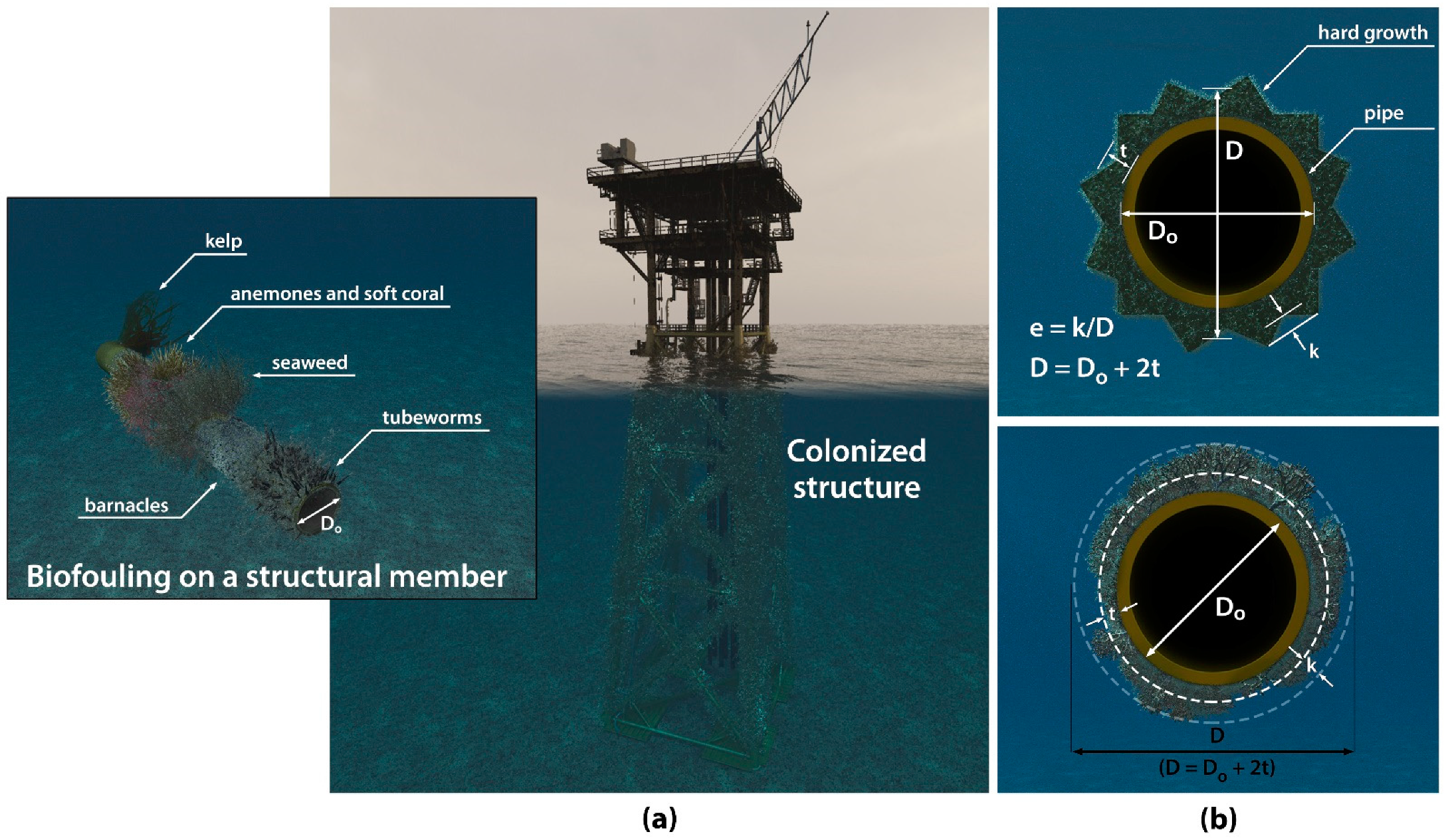
Figure 1. (a) Schematic view of soft and hard biofouling as per [2], and (b) definition of terms as per [11].
Jmse 09 01344 g001
Figure 2. Aksi3D device in lab and (a) tested in a wave tank at Ifremer; (b) U-shape end of the tip; (c) UN-SEA test site.
Jmse 09 01344 g002
Figure 3. Close-up view of the artificial colonization and board.
Jmse 09 01344 g003
Figure 4. Distribution (number) of heights of artificial colonization.
Jmse 09 01344 g004
Figure 5. Photographs of artificial colonization for flood light 58 cm (a,b. left) and spot light 65 cm (c,d. right). (a) Left camera, flood, 58 cm; (b) right camera, flood, 58 cm; (c) left camera, spot, 65 cm; (d) right camera, spot, 65 cm.
Jmse 09 01344 g005
Figure 6. UN-SEA-MDTC, two tanks 300 cm × 60 cm × 50 cm.
Jmse 09 01344 g006
Figure 7. Three photographs of a mooring chain fully coved by mussels on SEMREV test site (ac) and UN@SEA platform (d).
Jmse 09 01344 g007
Figure 8. Automatic specimen segmentation technique schematic.
Jmse 09 01344 g008
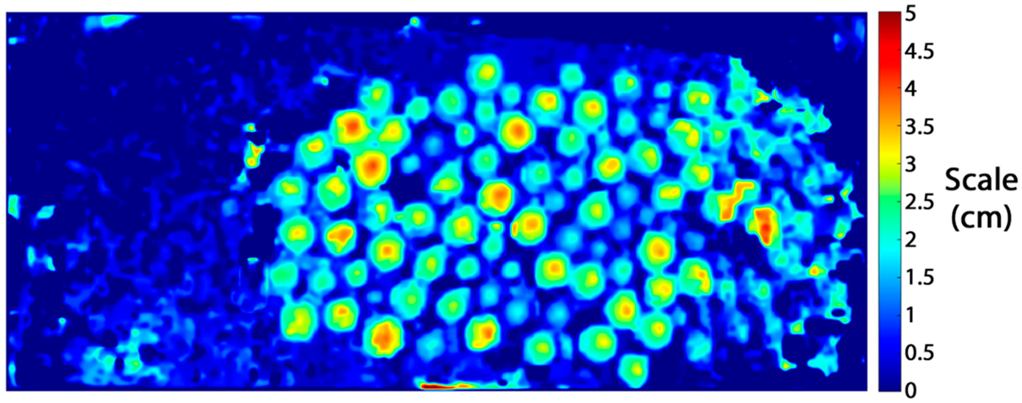
Figure 9. Scaled height map of the artificial specimen relative to the board (the elevation of the board is set to 0 cm).
Jmse 09 01344 g009
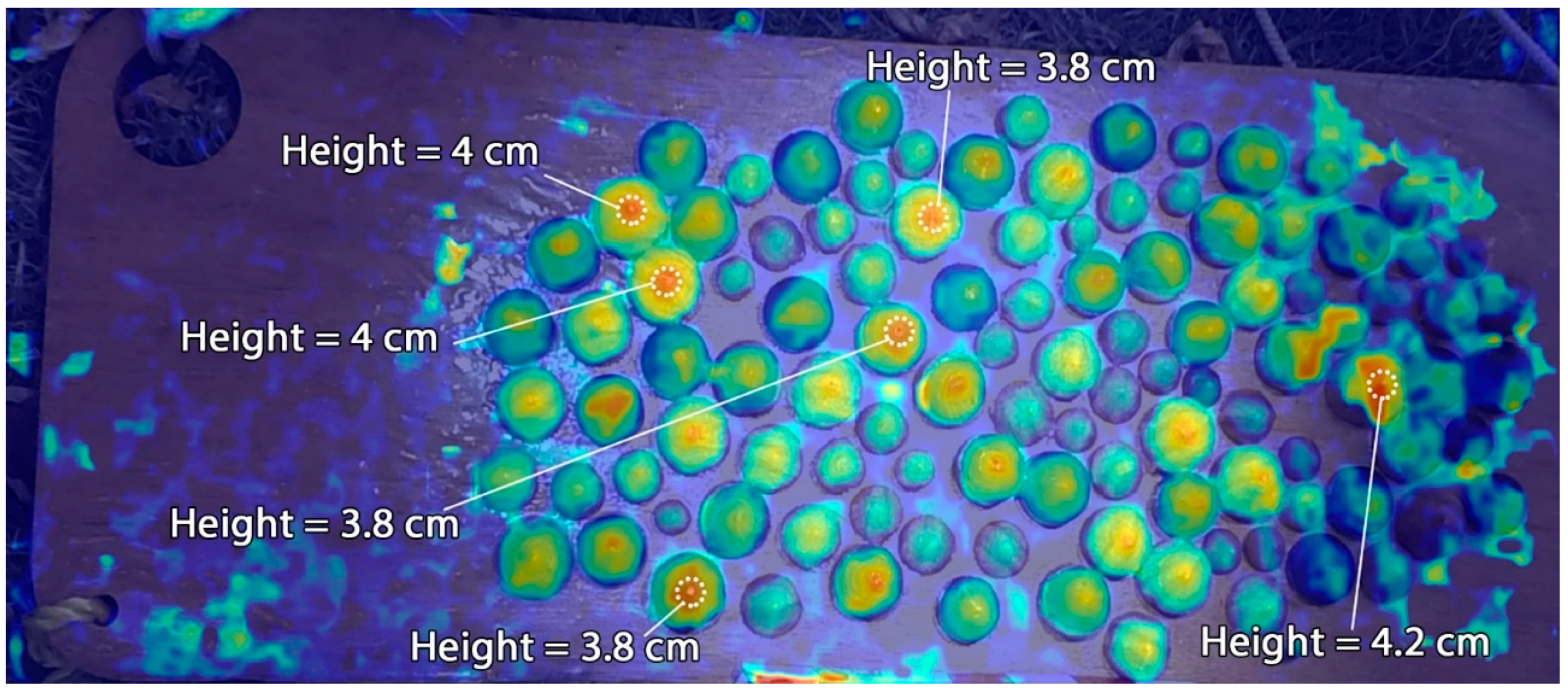
Figure 10. Overlay of the height map and the original image. The estimated heights for notable peaks are shown..
Jmse 09 01344 g010
Figure 11. Reconstructed image from left and right pictures corresponding to the conditions of Figure 3.
Jmse 09 01344 g011
Figure 12. Reconstructed images in two conditions, flood light 58 cm (a) and spot light 65 cm (b).
Jmse 09 01344 g012
Figure 13. Numerical mapping (a) and computation of specimen height (b).
Jmse 09 01344 g013
Figure 14. Three surfaces with the same roughness parameters (   R a = 0 , R m a = 0.797 , R s q = 1 , R s k   = 0 and R k u   = 3) with different fractal dimension DF = 9/4 (left), DF = 8/4 (middle), and DF = 11/4 (right).
Jmse 09 01344 g014
Figure 15. Distributions of roughness computed for each combination configuration, the left pane shows the Hisgotrem—58 cm/ 65 cm/ 100 cm/ 120 cm of Flood Lighting; the rightt pane shows the Hisgotrem—58 cm/ 65 cm/ 100 cm/ 120 cm of.Spot Lighting.
Jmse 09 01344 g015aJmse 09 01344 g015b
Figure 16. Results of segmentation of specimen for two configurations, 58 cm spot light (left) and 120 cm flood light (right).
Jmse 09 01344 g016
Figure 17. PoD, bias, and standard deviation of error for each protocol.
Jmse 09 01344 g017
Figure 18. Mean and standard deviation of the distributions (reference and protocols).
Jmse 09 01344 g018
Figure 19. Distribution of errors of measurement.
Jmse 09 01344 g019
Figure 20. ROC curves for each protocol.
Jmse 09 01344 g020
Figure 21. Roughness profiles R1, R2, and R3 as a function of pixel number.
Jmse 09 01344 g021
Figure 22. Boxplots for estimates of the fractal dimension from Gaussian random field samples with powered exponential covariance (16), using M = 5000 replicates for the three profiles: left R1, middle R2, right R3.
Jmse 09 01344 g022
Table 1. Methods considered to estimate the DF of a 1-D rough curve.
Method Q u ( . ) Scale   h Power Law
Madogram γ 1 ( h ) h : lag γ 1 ( h )   h 2 D F
Variogram γ 2 ( h ) h : lag γ 2 ( h ) h 4 2 D F
Periodogram S ( p ) spectral density p : frequency S ( p ) h 2 D F 5
Cube-count N ( h ) number of cubes h : with of cube N ( h ) h D F
Table 2. Skewness of the real distribution and the measured ones.
Ref.Light
m58 cm Flood58 cm Spot65 cm Flood65 cm Spot100 cm Flood100 cm Spot120 cm Flood120 cm Spot
0.040.50.30.31.40.71.21.11
Table 3. Relative errors (%) of the mean and standard deviation estimates.
58 cm
Flood Light
58 cm
Spot Light
65 cm
Flood Light
65 cm
Spot Light
100 cm
Flood Light
100 cm
Spot Light
120 cm
Flood Light
120 cm
Spot Light
Mean35352552515510
Standard deviation170145758520014510185
Table 4. Values of distance δ and corresponding detection threshold ad.
58 cm
Flood Light
58 cm
Spot Light
65 cm
Flood Light
65 cm
Spot Light
100 cm
Flood Light
100 cm
Spot Light
120 cm
Flood Light
120 cm
Spot Light
δ0.060.130.040.140.170.360.130.17
ad [cm]0.50.50.750.750.750.750.750.75
Table 5. Statistics for the roughness of the three trajectories.
Trajectory R1Trajectory R2Trajectory R3
Mean (cm)1.92.12.1
Standard deviation (cm)0.480.630.49
CoV (%)253023
Table 6. Classical roughness parameter estimates.
Profiles   R 1   R 2   R 3
Parameters
  R a 1.9222.1292.09
  R m a 0.4060.5110.3905
  R s q 0.4820.6340.488
  R s k 2.1682.4973.476
  R k u 0.1360.610.856
Table 7. Fractal dimension estimation.
Profiles R 1 R 2 R 3
Method
Madogram1.21021.19341.1872
Variogram1.27491.25341.2378
Cube-count1.23011.19391.1941
Periodogram1.48541.25571.1857
Publisher’s Note: MDPI stays neutral with regard to jurisdictional claims in published maps and institutional affiliations.