Coupling with the Embedded Boundary Method in a Runge-Kutta Discontinuous-Galerkin Direct Ghost-Fluid Method (RKDG-DGFM) Framework for Fluid-Structure Interaction Simulations of Underwater Explosions

Abstract

Solution of near-field underwater explosion (UNDEX) problems frequently require the modeling of two-way coupled fluid-structure interaction (FSI). This paper describes the addition of an embedded boundary method to an UNDEX modeling framework for multiphase, compressible and inviscid fluid using the combined algorithms of Runge-Kutta, discontinuous-Galerkin, level-set and direct ghost-fluid methods. A computational fluid dynamics (CFD) solver based on these algorithms has been developed as described in previous work. A fluid-structure coupling approach was required to perform FSI simulation interfacing with an external structural mechanics solver. Large structural deformation and possible rupture and cracking characterize the FSI phenomenon in an UNDEX, so the embedded boundary method (EBM) is more appealing for this application in comparison to dynamic mesh methods such as the arbitrary Lagrangian-Eulerian (ALE) method to enable the fluid-structure coupling algorithm in the fluid. Its limitation requiring a closed interface that is fully submerged in the fluid domain is relaxed by an adjustment described in this paper so that its applicability is extended. Two methods of implementing the fluid-structure wall boundary condition are also compared. The first solves a local 1D fluid-structure Riemann problem at each intersecting point between the wetted elements and fluid mesh. In this method, iterations are required when the Tait equation of state is utilized. A second method that does not require the Riemann solution and iterations is also implemented and the results are compared.

1. Introduction

Vulnerability to a near-field underwater explosion is an important performance metric in early-stage naval ship design that is frequently not considered. Severe damage including large deformation of hull structures and possible rupture, loss of water-tight integrity, failure of facilities and equipment, and personnel casualties are events that can occur as a result of underwater explosions of this category [1,2]. Near-field UNDEX is a problem that can involve significant fluid-structure interaction. The fluid loads including primary shock waves and blast deform the structure in the vicinity of the explosion. The deforming structure, in turn, interacts with the fluid including the formation and closure of local cavitation. The physics of this FSI problem is complex and existing mathematical models require significant computational effort and detail, typically not considered in early-stage design. Full scale experiments with near-field UNDEX typically cannot be conducted because of their expense and damage to the ship [1,2,3]. A well-developed and computationally cost-efficient algorithm to perform UNDEX simulations is needed, especially in early-stage ship design.

In the framework described in this paper, the flow in an UNDEX is modeled as multiphase, compressible and inviscid using the Euler equations. The fluid governing equations are solved using a hybrid framework of algorithms. These algorithms include the Runge–Kutta and discontinuous-Galerkin methods as the discretization scheme of the fluid equations, and the level-set and direct ghost-fluid methods as the multiphase approach. The discontinuities in the solution field, i.e., the shock and rarefaction wave front, must be tracked accurately while the total variation diminishing property is enforced. This is achieved using a slope limiter. A non-reflecting boundary condition (NRBC) is also implemented so that a smaller domain can be used to save computing memory and reduce effort. A computational fluid dynamics solver is developed based on a combination of these algorithms in a hybrid framework. The framework has been assessed in multiple cases. This paper describes the continuing development of this framework and solver. Details are provided in two preceding papers [4,5].

A Eulerian mesh is used in the fluid domain and a Lagrangian mesh is used in the structural domain. The former is fixed in space while the latter is fixed in the material [6]. Numerical techniques are therefore needed to treat the interaction of the two domains. In general, numerical techniques for this purpose can be categorized into two classes: dynamic mesh methods and the embedded boundary method. In dynamic mesh methods, a body-conforming fluid domain is built and discretized with a structured/unstructured mesh depending on the shape of the structural object. The fluid mesh needs to deform according to the motion and deformation of the structure throughout the simulation. Coupled Eulerian-Lagrangian (CEL) and Arbitrary Lagrangian-Eulerian (ALE) are typical dynamic mesh methods. The CEL method uses Lagrangian and Eulerian meshes for the structural and fluid domains, respectively, and a complex mapping algorithm to exchange computational information at the interface. The complexities of the algorithm can cause significant error if there is overlap at the interface of the two domains [7,8]. The ALE method allows the fluid mesh to move according to the motion and deformation of the structural object. In this method, mesh-smoothing and remapping is needed at each time step during the simulation. Mesh distortion can be avoided as the mesh is allowed to move independent of the motion of the fluid material [9,10,11,12,13,14,15]. This method features high accuracy at the fluid-structure interface as the fluid mesh is always body-conforming. High mesh resolution is thus achievable for boundary layers if the flow is viscous. However, special care must be taken with the mesh-smoothing and re-mapping algorithm when the motion and deformation of the structure is very large. In problems such as UNDEX, structural cracking and rupture may occur which causes a topological challenge that the ALE method cannot manage.

The embedded boundary method was first developed and used in the simulation of blood flows in elastic heart valves and has since gained significant attention in CFD and FSI simulations [16]. This method avoids challenges that are experienced with the dynamic mesh method. Meshing of the fluid domain is simplified especially for inviscid flow because the mesh does not need to be refined towards the wall in order to satisfy the boundary layer and possibly ${\mathrm{U}}^{+}$ and ${\mathrm{y}}^{+}$ requirements. Shape of the fluid domain can thus be rectangular and can be discretized using a Cartesian-structured mesh which is preferable for the stability of computation. Mesh-smoothing, mesh-remapping and other necessary algorithms needed in the fluid solver are not necessary, which significantly increases the computational efficiency of the FSI simulation. Large motion and deformation of the structural object cause no issues for the fluid because the fluid mesh is fixed in space and indirectly able to track the embedded wall shape [17]. Structural cracking and ruptures can be treated without the topological challenges in the dynamic mesh method [18].

Many researchers are using the embedded boundary method with compressible and inviscid flows because of its appealing advantages over the dynamic mesh method in simulations of FSI problems that feature large motion and deformation and other topological challenges. Different types of implementation of the EBM have been developed and applied. Liu et al. [19,20] used a ghost-cell type of immersed boundary method that operates on an adaptive Cartesian fluid grid integrated with a Runge-Kutta discontinuous-Galerkin fluid algorithm. Tracking of the embedded surface is based on an image point ghost-cell method. A closed row of solid cells near the embedded surface is identified and then the wall boundary condition is implemented. Performance of simulations using this type of EBM is yet to be validated by experiments featuring large motion and deformation of structural objects. Xiao et al. [21] used an embedded boundary method with a cut-cell approach coupled with both finite volume and discontinuous-Galerkin fluid algorithms. In their method, multiple approaches are proposed to overcome the excessive stable time step restrictions imposed by the cut-cells. Additional nodes are introduced on the element faces abutting the solid boundary. Faces are curved by projecting the introduced nodes on the boundary. Accuracy is increased at the cost of computational efficiency. Ralf et al. [22] used an embedded boundary method based on a diffused boundary technique. This method is essentially a cut-cell approach of a different type. The staircase approximation of the boundary is alleviated by using the dynamic mesh adaptation technique. Performance of simulations using this type of EBM is yet to be validated by experiments. Zhang et al. [23] coupled the Runge-Kutta discontinuous-Galerkin fluid algorithm with an EBM that includes a tracking algorithm to solve 2D problems.

Wang and Farhat [18,24] developed a unique implementation of the embedded boundary method in FSI simulations where both the compressible and inviscid flow and the deformable structure possess significant response, such as in underwater implosions and explosions. In their work, two algorithms for tracking the embedded wetted wall on a structured or unstructured CFD grid are proposed: the projection-based and the collision-based algorithms. The former features high efficiency of computation, but can only track a closed interface that is completely submerged in the fluid domain. The closed-interface restriction is relaxed in the collision-based approach, but the simulation is much slower [18]. The application described in this paper adjusts the projection-based algorithm so that the closed-interface restriction is lifted while maintaining its efficiency. Mathematical exceptions are repaired so that edge cases are removed. The algorithm is further modified so that it is less complicated to understand and implement. Another method proposed by Wang [18] is used to enforce the appropriate value of fluid velocity at the wall and recover the fluid pressure by solving a local 1D fluid-structure Riemann problem at each intersecting point between the wetted elements and fluid mesh. This approach of implementing the fluid-structure wall boundary condition was a significant contribution in Wang and Farhat’s work [18]. This method is shown to maintain high accuracy of the FSI simulation at the fluid-structure boundary, but can take longer to run if the Tait equation of state is used where iteration is needed since there is no explicit analytic solution to the 1D Riemann problem. A different approach which does not involve the Riemann solution and iterations is used in this paper. Simulation results using both this approach and the Riemann solution approach are compared and assessed by experiment presented later in this paper. The approach that does not involve a Riemann solution and iterations is preferable in early-stage ship design, if it is sufficiently accurate compared with the approach that involves Riemann solution and iterations.

Other methods and tools for FSI simulation of UNDEX problems exist in the literature, such as LS_DYNA, which uses the finite element method as the fluid discretization scheme and the ALE method as the interface between the fluid and structural domains. Work using this method includes Klenow [2], Webster [25], and Sjostrend [26]. Noorpoor, et al. [27] used OpenFOAM, which uses the finite volume method as the fluid discretization scheme. Farhat, et al. [28] developed and used Aero-f, a finite-volume-based fluid solver, coupled with Aero-s, a finite-element-based structural solver, and performed UNDEX simulations of different configurations. Early research performed by the author’s research group, including Webster [25], indicated that LS_DYNA did not successfully enforce the non-reflecting boundary condition. Also, there was significant pressure oscillation in its prediction of the UNDEX shock wave profile. The discontinuous-Galerkin (DG) method relaxes the connectivity requirement between elements so it is preferrable over finite volume (FV) methods in simulating problems with discontinuities, such as UNDEX shock waves. Therefore, the author decided to develop a hybrid framework of CFD numerical methods that incorporates the DG method as the fluid discretization scheme vice one of these finite-volume methods.

In summary, the following contributions were made to satisfy the objectives of this research:

(1)

Developed an improved projection-based EBM which lifts the closed-interface restriction, and identifies and corrects problems that could cause edge cases; further simplified the algorithms to improve their computational efficiency; and applied the improved projection-based EBM to fluid-structure interaction simulations of UNDEX problems.

(2)

Developed a hybrid framework of fluid algorithms to integrate the numerical methods; and coupled it with finite-element-based structural methods to perform UNDEX simulations for the purpose of early-stage ship design.

(3)

Used the methods to simulate different configurations of UNDEX problems and assessed the simulations by experiment.

Section 1 of this paper introduces the background and related research regarding the hybrid framework of algorithms used to solve the fluid flow in an UNDEX, the embedded boundary method, and the importance of the embedded boundary method in this framework of fluid algorithms. Section 2 describes the mathematics involved in the embedded boundary method as adapted in this work, with a focus on the necessary adjustments made to improve its performance. Section 3 describes and applies the embedded boundary method coupled with the previously-developed CFD solver in the hybrid framework of algorithms. Details of the development of the CFD solver is documented in preceding papers [1,2].

Ref. [4] discusses the development of the Runge-Kutta discontinuous-Galerkin framework of fluid discretization, the verification of the solver developed based on this framework, the implementation of slope limiter, and the enforcement of the non-reflecting boundary condition (NRBC). Its highlights are

(1)

Documented a straightforward method for multi-dimensional discretization of compressible and inviscid fluid governing equations (the Euler equations) using a modal DG method.

(2)

Performed order-of-accuracy verification on the developed single and multi-dimensional UNDEXVT solvers with different formal orders of accuracy; observed order of accuracies match the formal order of accuracy.

(3)

Simulated multiple cases that possess near-field and early-time UNDEX features; compared simulation results with analytic solutions, experiments and simulations using other algorithms; proved the applicability of this hybrid framework.

(4)

Compared different methods for enforcing the NRBC; selected an optimized method which is developed by the author.

(5)

FSI simulations of near-field and early-time UNDEX problems can be achieved once the framework is coupled with the embedded boundary method (EBM).

Ref. [5] introduces the treatment of multi-phase fluid using the level-set and direct Ghost-Fluid method. Its highlights are

(1)

Presented the direct Ghost-Fluid method (DGFM); extended two-dimensional DGFM to three-dimensions; implemented and compared three algorithms for enforcing the interface conditions.

(2)

Compared simulations with analytic and experimental results in a series of benchmark problems.

(3)

The DGFM decreases the density diffusion across the interface between the explosive gaseous products and the surrounding water; spurious pressure oscillations at the material interface are therefore minimized.

(4)

The DGFM is also successfully applied to the simulation of an explosion inside a rigid tube filled with distilled water.

2. Embedded Boundary Method Algorithms

Tracking of the embedded wetted surface and the implementation of the fluid-structure wall boundary condition are two problems of interest in an embedded boundary method. The tracking algorithm is illustrated using specific examples to demonstrate how it works with necessary adjustments. After this, two approaches for performing the implementation of the fluid-structure wall boundary condition are introduced. Comparisons between these approaches are made in the test cases described in Section 3.

2.1. Embedded Wetted Surface Tracking Algorithm

Embedded wetted surfaces of two different geometrical shapes are used to illustrate the EBM tracking algorithm with variations used in this work. These surfaces do not have a closed-interface and are not fully submerged in the fluid domain. This projection-based tracking algorithm was proposed by Wang and Farhat’s work [18] and improved by the authors.

(a)

wetted surface A: a rectangular barge floating on the free surface;

(b)

wetted surface B: a wedge whose cross-sectional shape consists of a rectangle and a triangle;

Configurations of these two wetted surfaces embedded in the fluid domain are shown in Figure 1.

Nomenclature used to describe the tracking algorithm is listed in

Table 1. Nomenclature used to describe the tracking algorithm.

Symbols	Notes
${\mathrm{D}}_{\mathrm{h}}$	The fluid mesh
${\mathrm{D}}_{\mathrm{h}}^{\mathrm{E}}$	The structural mesh
${\mathrm{V}}_{\mathrm{ijk}}$	Cell $\left(\mathrm{i},\mathrm{j},\mathrm{k}\right)$’s center of the fluid mesh
${\mathrm{b}}_{\mathrm{ijk}}$	Cell $\left(\mathrm{i},\mathrm{j},\mathrm{k}\right)$’s axis-aligned bounding box
${\mathrm{E}}_{\mathrm{n}}$	Element $\mathrm{n}$ of the structural mesh
${\mathrm{b}}_{\mathrm{n}}$	Element $\mathrm{n}$’s axis-aligned bounding box
${\mathrm{S}}_{\mathrm{ijk}}$	The status of cell $\left(\mathrm{i},\mathrm{j},\mathrm{k}\right)$’s center of the fluid mesh, 0 indicates it resides in the fluid, 1 indicates it does not reside in the fluid, −1 indicates it is to be determined.
${\mathrm{V}}_{\mathrm{ijk}}^{\prime }$	The closest point on the structural mesh to cell $\left(\mathrm{i},\mathrm{j},\mathrm{k}\right)$

.

The algorithm can be summarized in six steps as follows:

Step 1. Break the quadrilateral wetted elements into triangular elements, as shown in Figure 2.

Step 2. Compute outward normal vectors pointing towards fluid, as shown in Figure 3.

Step 3. Denote the fluid mesh as ${\mathrm{D}}_{\mathrm{h}}$ and the embedded wetted mesh as ${\mathrm{D}}_{\mathrm{h}}^{\mathrm{E}}$. ${\mathrm{D}}_{\mathrm{h}}$ in these configurations is a Cartesian structured mesh, but it could be any type, structured or unstructured. For each cell center ${\mathrm{V}}_{\mathrm{ijk}}$, an axis-aligned bounding box ${\mathrm{b}}_{\mathrm{ijk}}$ is constructed, connecting its neighboring cell centers as vertices. Also, for each triangle ${\mathrm{E}}_{\mathrm{n}}$ of the embedded wetted mesh, an axis-aligned bounding box ${\mathrm{b}}_{\mathrm{n}}$ is constructed which is the smallest box that can enclose the triangle.

Step 4. Set the status of each fluid cell of ${\mathrm{D}}_{\mathrm{h}}$ as ${\mathrm{s}}_{\mathrm{ijk}}=0$. Determine for each cell center ${\mathrm{V}}_{\mathrm{ijk}}$ of ${\mathrm{D}}_{\mathrm{h}}$, whether it is close enough to the embedded wetted surface ${\mathrm{D}}_{\mathrm{h}}^{\mathrm{E}}$. If it is close enough to ${\mathrm{D}}_{\mathrm{h}}^{\mathrm{E}}$, the point on ${\mathrm{D}}_{\mathrm{h}}^{\mathrm{E}}$ that is closest to ${\mathrm{V}}_{\mathrm{ijk}}$, ${\mathrm{V}}_{\mathrm{ijk}}^{’}$, must be located. The status of ${\mathrm{V}}_{\mathrm{ijk}}$, ${\mathrm{s}}_{\mathrm{ijk}}$, is also determined. ${\mathrm{s}}_{\mathrm{ijk}}=0$ indicates that ${\mathrm{V}}_{\mathrm{ijk}}$ actually resides in the fluid while ${\mathrm{s}}_{\mathrm{ijk}}=1$ indicates that ${\mathrm{V}}_{\mathrm{ijk}}$ does not reside in the fluid. This is achieved in three sub-steps discussed in detail in the third appendix of the author’s dissertation [29], along with the adjustment made in Step 4 so that the closed-interface limitation is removed. Mathematical exceptions in Step 4 are also fixed so that edge situations in which the algorithm fails to track the embedded surface are removed. The outcome of Step 4 is illustrated in Figure 4. Blue denotes the cell center that resides in the fluid while red denotes the cell center that does not reside in the fluid.

Step 5. Determine whether remaining cells in the mesh reside in the fluid or not using a flood-fill algorithm [30]. The outcome of this step is illustrated in Figure 5. Blue denotes a cell center that resides in the fluid while red denotes a cell center that does not reside in the fluid.

Step 6. Loop over the whole CFD domain, ${\mathrm{D}}_{\mathrm{h}}$, and find all neighboring-cell pairs $\left({\mathrm{V}}_{\mathrm{ijk}},{\mathrm{V}}_{\mathrm{i}+1,\mathrm{j},\mathrm{k}}\right)$, $\left({\mathrm{V}}_{\mathrm{ijk}},{\mathrm{V}}_{\mathrm{i},\mathrm{j}+1,\mathrm{k}}\right)$ and $\left({\mathrm{V}}_{\mathrm{jik}},{\mathrm{V}}_{\mathrm{i},\mathrm{j},\mathrm{k}+1}\right)$ whose status pair ${\mathrm{s}}_{\mathrm{ijk}}\ne {\mathrm{s}}_{\mathrm{i}+1,\mathrm{j},\mathrm{k}}$, ${\mathrm{s}}_{\mathrm{ijk}}\ne {\mathrm{s}}_{\mathrm{i},\mathrm{j}+1,\mathrm{k}}$ and ${\mathrm{s}}_{\mathrm{ijk}}\ne {\mathrm{s}}_{\mathrm{i},\mathrm{j},\mathrm{k}+1}$. Pairs of this kind indicate fluid-structure intersecting edges. The intersecting point on the embedded wetted surface, ${\mathrm{D}}_{\mathrm{h}}^{\mathrm{E}}$, is then located. The outcome of this step is illustrated in Figure 6. The red points are the intersecting points computed in this step.

2.2. Implementation of the Fluid-Structure Wall Boundary Condition in the Fluid Calculation

Wang et al. [18,24] proposed an approach to implement the fluid-structure wall boundary condition in the fluid solver by solving a local 1D fluid-structure Riemann problem at each intersecting point between the wetted elements and fluid mesh. The fluid velocity at the wall is enforced and thus the fluid pressure at the wall is recovered through the solution of this problem analytically. Using a 2D mesh to illustrate, this approach is summarized as follows.

Cell pair $\left(\mathrm{i},\mathrm{j},\mathrm{k}\right)$ and $\left(\mathrm{i}+1,\mathrm{j},\mathrm{k}\right)$ constitutes an intersecting pair with the left cell residing in the fluid. This is tracked by the algorithm described in Section 2.1. Wall velocity ${\overrightarrow{\mathrm{V}}}_{\mathrm{S}}$ at the intersecting point (the solid red triangle in Figure 7) is computed using the nodal velocity from the structural solver and the shape functions or the barycentric coordinates of the intersecting point. A local 1D fluid-structure Riemann problem with a prescribed velocity at the wall boundary is formulated.

$$\frac{\partial }{\partial \mathrm{t}}\left\{\begin{array}{c}\mathsf{\rho }\\ \mathsf{\rho }\mathrm{u}\\ \mathsf{\rho }\mathrm{E}\end{array}\right\}+\frac{\partial }{\partial \mathrm{s}}\left\{\begin{array}{c}\mathsf{\rho }\mathrm{u}\\ \mathsf{\rho }{\mathrm{u}}^2+\mathrm{p}\\ \mathsf{\rho }u\left(\mathrm{E}+\frac{\mathrm{p}}{\mathsf{\rho }}\right)\end{array}\right\}=0\mathrm{where}\mathrm{s}\in \left(-\infty ,{\mathrm{u}}_{\mathrm{wall}}\mathrm{t}\right)\mathrm{and}\mathrm{t}\in \left(0,\Delta \mathrm{t}\right)$$

(1)

$$\mathrm{Initial}\mathrm{conditions}:\left\{\begin{array}{c}\mathsf{\rho }\left(\mathrm{s},0\right)={\mathsf{\rho }}_{\mathrm{ijk}}\\ u\left(\mathrm{s},0\right)={\overrightarrow{\mathrm{V}}}_{\mathrm{ijk}}·\left(-{\hat{\mathrm{n}}}_{\mathrm{m}}\right)\\ \mathrm{p}\left(\mathrm{s},0\right)={\mathrm{p}}_{\mathrm{ijk}}\end{array}\right.\mathrm{where}\mathrm{s}\in \left(-\infty ,0\right)$$

(2)

$$\mathrm{Boundary}\mathrm{conditions}:\mathrm{u}\left(\mathrm{s}={\mathrm{u}}_{\mathrm{wall}}\mathrm{t},\mathrm{t}\right)={\mathrm{u}}_{\mathrm{wall}}={\overrightarrow{\mathrm{V}}}_{\mathrm{S}}·\left(-{\hat{\mathrm{n}}}_{\mathrm{m}}\right)$$

(3)

The so-called “star state” of primitive variables is computed through the solution of this problem [31]. Primitive variables at the right facet (the unfilled red triangle in Figure 7, denoted as the M-state) of the fluid cell $\left(\mathrm{i},\mathrm{j},\mathrm{k}\right)$ are evaluated by

$$\left\{\begin{array}{c}{\mathsf{\rho }}_{\mathrm{M}}={\mathsf{\rho }}^{*}\\ {\overrightarrow{\mathrm{V}}}_{\mathrm{M}}=({\overrightarrow{\mathrm{V}}}_{\mathrm{ijk}}-({\overrightarrow{\mathrm{V}}}_{\mathrm{ijk}}·{\hat{\mathrm{n}}}_{\mathrm{m}}){\hat{\mathrm{n}}}_{\mathrm{m}})+{\mathrm{u}}_{\mathrm{wall}}\left(-{\hat{\mathrm{n}}}_{\mathrm{m}}\right)\\ {\mathrm{p}}_{\mathrm{M}}={\mathrm{p}}^{*}\end{array}\right.$$

(4)

So that flux at the right facet can be computed. This approach has high accuracy at the fluid-structure boundary, but can take longer, especially if the Tait equation of state is used where iteration is needed. A different approach can be used to save time as may be important in the early-stage ship design process. In this approach, the first and third terms in Equation (4) are replaced by the fluid state at cell $\left(\mathrm{i},\mathrm{j},\mathrm{k}\right)$.

$$\left\{\begin{array}{c}{\mathsf{\rho }}_{\mathrm{M}}={\mathsf{\rho }}_{\mathrm{ijk}}\\ {\overrightarrow{\mathrm{V}}}_{\mathrm{M}}=({\overrightarrow{\mathrm{V}}}_{\mathrm{ijk}}-({\overrightarrow{\mathrm{V}}}_{\mathrm{ijk}}·{\hat{\mathrm{n}}}_{\mathrm{m}}){\hat{\mathrm{n}}}_{\mathrm{m}})+{\mathrm{u}}_{\mathrm{wall}}\left(-{\hat{\mathrm{n}}}_{\mathrm{m}}\right)\\ {\mathrm{p}}_{\mathrm{M}}={\mathrm{p}}_{\mathrm{ijk}}\end{array}\right.$$

(5)

The extent to which this approach decreases the accuracy of simulation is investigated in Section 3.

3. Assessment

In this section, three simulations for near-field and early-time underwater explosions using the CFD solver with embedded boundary method in the hybrid framework of algorithms (Runge-Kutta, discontinuous-Galerkin, level-set, direct ghost-fluid) coupled with the Abaqus/Explicit structural solver are described. MpCCI is used to couple the fluid and structural solvers [32]. The simulations are assessed using experimental results. The first case is an explosion inside a water-filled Aluminum tube. The second case is an explosion near a steel plate in a blast test. The third case is an explosion near a square plate made of composite material.

Case 1 investigates an internal explosion inside a water-filled Aluminum tube. This experiment was performed by Sandusky et al. [33,34]. A 3 g PETN charge is placed at the center of the tube that is made of Aluminum 5086. A thin plastic sheet is used to seal the bottom of the tube. The top of the tube is left open. A pressure gauge is installed at the inner center of the tube wall to measure the pressure-time history [15,35,36]. The arrangement of this experiment is illustrated in Figure 8. Time histories of fluid pressure, wall velocity and deflection are sampled at the inner center of the wall as shown in Figure 8.

In the fluid simulation, the initial conditions are set up as in Figure 9. Making use of the symmetry of this configuration, a rectangular domain $\left[0.0,6.0\times {10}^{-2}\right]\mathrm{m}\times \left[0.0,8.9\times {10}^{-2}\right]\mathrm{m}\times \left[0.0,6.0\times {10}^{-2}\right]\mathrm{m}$ that represents 1/8 of the whole geometry is discretized with a $60\times 89\times 60$ Cartesian structured grid. In the structural simulation, the initial conditions are set up as in Figure 10. Making use of the symmetry of this configuration, a 1/8 domain is built and discretized with a $40\times 52$ Cartesian structured grid. The simulation is run to a final time of $2.0\times {10}^{-4}$ seconds.

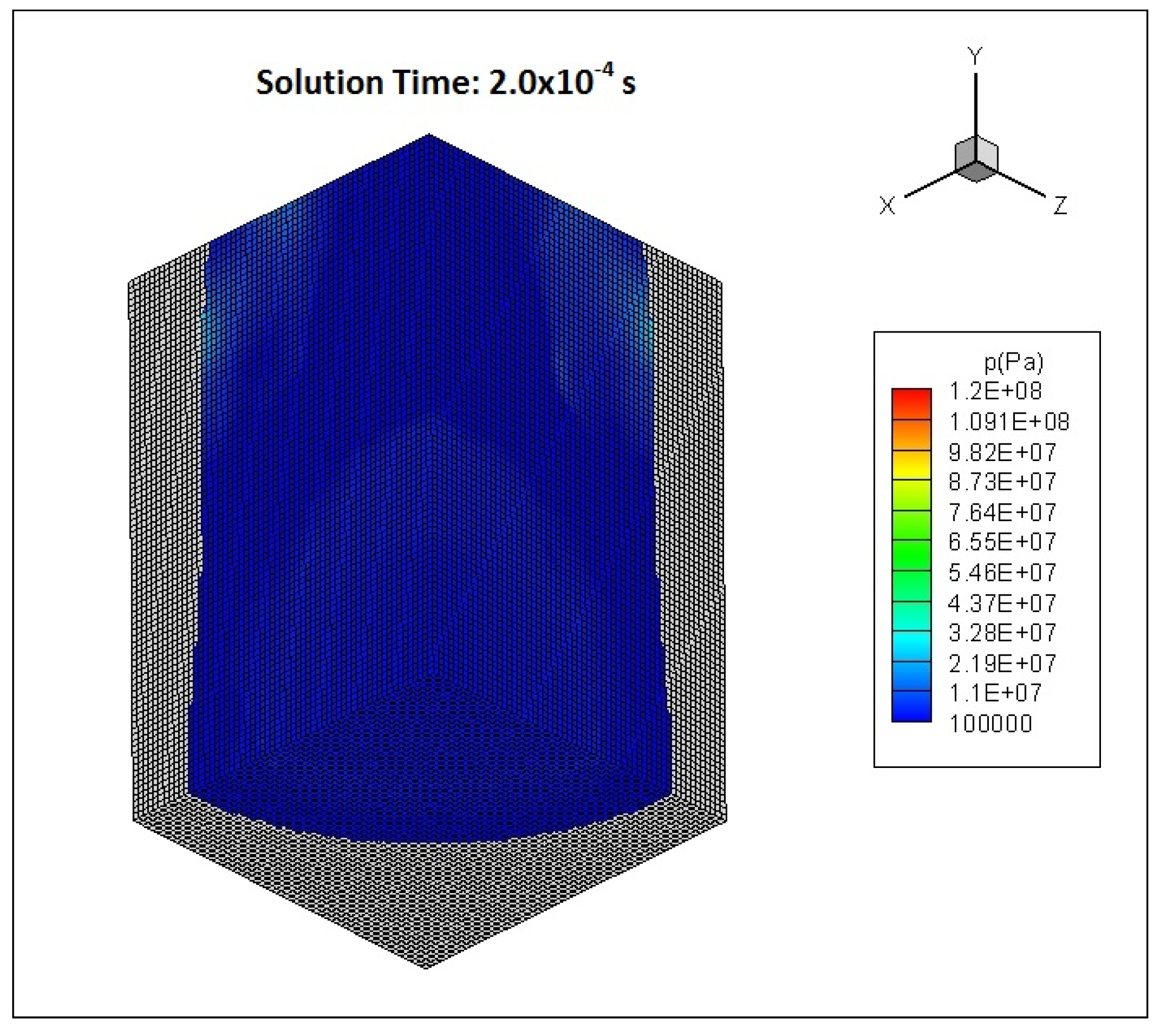
The deformations of the fluid domain and the structure are displayed in Figure 11 and Figure 12, respectively. Contours of fluid pressure every $1.5\times {10}^{-5}\mathrm{s}$ are displayed in Figure 13.

The simulated deformation and velocity of the inner center of the wall are plotted in Figure 14 and Figure 15, respectively, using both approaches of implementing the fluid-structure slip-wall boundary condition, and are compared with the experiment. Fluid pressure at the same location are plotted in Figure 16 showing results for experiment and simulations using both approaches of slip-wall boundary implementation.

When the explosion occurs, a shock wave is generated which impacts the wall of the cylinder. When loaded by the primary shock wave, the wall deforms outward. Because the compressibility of water is relatively small, it cannot sustain much traction, so that the extra volume created by the deformation of the wall reduces its density and pressure in the vicinity of the deformed wall. A local cavitation zone is thus formed. This cavitation zone gradually disappears as the acceleration of the wall outward decreases and the surrounding water rushes into the local cavitation zone.

The shock that reflects off the wall travels back and eventually comes in contact with the explosive gas and they interact with each other, creating an expansion zone that lowers the density and pressure of the fluid and thus forms another cavitation zone [15,36] as marked in the fourth contour of Figure 13 using a yellow circle. This cavitation collapses as well and forms a new shock wave that impacts the wall again [15,36], as illustrated in the sixth contour of Figure 13. The wall then deforms with acceleration again. This process repeats until the energy of the fluid gradually decays and eventually the deformation of the structure stabilizes around a permanent value of deformation.

Figure 14 indicates that the deflection of the wall is predicted well by the simulation. The simulation matches closely with the experiment. The deflection of structure and its associated stress are important in early-stage ship design.

Figure 15 indicates that the velocity of the wall deformation is predicted reasonably well by the simulation. The 1st peak velocity differs from the experiment, possibility because the velocity is calculated by the difference between coordinates at successive time steps, divided by the time step size. A greater mesh refinement would minimize this difference. Timing of the 2nd peak velocity, occurring due the 2nd shock wave formed after the closure of the cavitation in the expansion zone, is earlier in the simulation (around $7.5\times {10}^{-5}$ s) than in the experiment (around $9.0\times {10}^{-5}$ s). Its peak value is higher than that in the experiment. The reason for these is because the geometry of the wall boundary is not perfectly conformed by the 3D fluid mesh in the EBM. The domain in the 3D fluid has flat sides between nodes at the fluid-wall boundary, but is actually curved. The embedded structural wall penetrates the fluid mesh at different angles along the perimeter. This leads to an asymmetry along the perimeter about the center axis which can be seen in the sixth contour of Figure 13. This problem could be alleviated with greater mesh refinement, but it is sufficient for the early-stage ship design application where it is preferrable to keep the simulation on a personal computer (PC) and limit the calculation time. Further mesh refinement is time prohibitive for this application where many designs and explosion scenarios may need to be evaluated in a ship design process without high performance computers (HPC).

Figure 16 indicates that the pressure at the inner center of the wall is predicted reasonably well by the simulation in that the overall behavior matches with experiment. The 1st peak pressure is underpredicted by the simulation compared with the experiment, and its rise is less steep. The local cavitation occurs earlier in the simulation than in the experiment. The reason for these differences is because in the embedded boundary method, the wall velocity at the intersecting points on the embedded wetted wall (like the solid red triangle in Figure 7) is used to compute the primitive variables of the fluid flow. When the fluid variables are computed, the flux is computed and implemented on the cell facets that are fixed in space (like the unfilled red triangle in Figure 7). With limited mesh refinement, the fluid senses that the structure is moving faster than it actually is. Timing of the 2nd peak pressure is earlier in the simulation (around $7.5\times {10}^{-5}$ s) than in the experiment (around $9.0\times {10}^{-5}$ s) and its peak value is higher in the simulation than in the experiment. The reason for this is also likely limited mesh refinement.

A comparison of the simulations using the two different wall boundary approaches indicates that the approach that does not involve Riemann solution and iterations do not substantially reduce the effectiveness of the simulation.

Table 2. Experiment-simulation differences using two different approaches of implementing wall boundary.

$\mathbf{Experiment}-\mathbf{Simulation}\mathbf{Difference}\text{—}\mathbf{Computed}\mathbf{as}\mathbf{an}\mathbf{Integrated}\mathbf{Error}\mathbf{Measure}\mathbf{over}\mathbf{the}\mathbf{Duration}\mathbf{of}\mathbf{Time}\mathbf{History},\mathbf{Using}{\mathbf{L}}_1\mathbf{Norm}$	p (Pa)	u (m)	v (m/s)
Wall boundary implementation involving iterations	$7.3880\times {10}^7$	$9.9731\times {10}^{-5}$	$1.2645\times {10}^1$
Wall boundary implementation not involving iterations	$7.6666\times {10}^7$	$1.1767\times {10}^{-4}$	$1.3280\times {10}^1$

indicates that the experiment-simulation differences using the two approaches are very small. The experiment-simulation differences are computed as an integrated error measure over the duration of time history, using ${\mathrm{L}}_1$ norm. Because of this, the approach that does not involve iterations is preferable when efficiency is required, such as in an early-stage ship design.

Table 2 also indicates that simulations using either approach of implementing the wall boundary provide results of sufficient accuracy. The magnitude of peak pressure in the experiment is in the order of $1.0\times {10}^8$ Pa, while the experiment-simulation difference using either approach is in the order of $1.0\times {10}^7$ Pa. The magnitude of peak velocity in the experiment is in the order of $1.0\times {10}^2$ m/s, while the experiment-simulation difference using either approach is in the order of $1.0\times {10}^1$ m/s. The magnitude of deformation at around $1.25\times {10}^{-4}$ s, when the deformation is about to be stabilized, is in the order of $1.0\times {10}^{-3}$ m, while the experiment-simulation difference using either approach is in the order of $1.0\times {10}^{-4}$ m. These errors are all approximately 10%, which is acceptable for early-stage ship design.

In the above simulations, the Zerilli-Armstrong constitutive model [33] is used for modeling of the structural elasticity and plasticity:

$$\mathsf{\sigma }=\left\{\begin{array}{cc}\mathrm{E}\mathsf{\epsilon }& \mathrm{elastic}\\ {\mathsf{\sigma }}_{\mathrm{Y}}+\mathrm{B}\sqrt{{\mathsf{\epsilon }\mathrm{e}}^{-\mathsf{\beta }\mathrm{T}}}& \mathrm{plastic}\end{array}\right.$$

(6)

Material properties of Al 5086 such as $\mathrm{E}$ and ${\mathsf{\sigma }}_{\mathrm{Y}}$ and other material parameters such as $\mathrm{B}$, $\mathsf{\beta }$ and $\mathrm{T}$ are from [33]. In a separate simulation, the power law isotropic elasto-plastic model [37] is used instead and results are compared with the above simulations:

$$\mathsf{\sigma }=\left\{\begin{array}{cc}\mathrm{E}\mathsf{\epsilon }& \mathrm{elastic}\\ {\mathsf{\sigma }}_{\mathrm{Y}}{\left(\frac{\mathrm{E}}{{\mathsf{\sigma }}_{\mathrm{Y}}}\mathsf{\epsilon }\right)}^{\mathrm{N}}& \mathrm{plastic}\end{array}\right.$$

(7)

Material parameters of Al 5085 in the power law isotropic elastoplastic mode are from [37]. Results for the structural deformation and velocity of the inner center of the wall and the fluid pressure at this location are plotted and compared with the experiment in Figure 17, Figure 18 and Figure 19, respectively. Experiment-simulation differences for simulations using both constitutive models are shown in

Table 3. Experiment-simulation differences using the two different constitutive models.

$\mathbf{Experiment}-\mathbf{Simulation}\mathbf{Difference}\text{—}\mathbf{Computed}\mathbf{as}\mathbf{an}\mathbf{Integrated}\mathbf{Error}\mathbf{Measure}\mathbf{over}\mathbf{the}\mathbf{Duration}\mathbf{of}\mathbf{Time}\mathbf{History},\mathbf{Using}{\mathbf{L}}_1\mathbf{Norm}$	p (Pa)	u (m)	v (m/s)
UNDEXVT/Abaqus: Zerilli-Armstrong constitutive	$7.6666\times {10}^7$	$1.1767\times {10}^{-4}$	$1.3280\times {10}^1$
UNDEXVT/Abaqus: power law isotropic elasto-plastic	$7.6630\times {10}^7$	$1.2349\times {10}^{-4}$	$1.3224\times {10}^1$

. The experiment-simulation differences are computed as an integrated error measure over the duration of time history using the ${\mathrm{L}}_1$ norm.

These comparisons indicate that the choice of constitutive models does not significantly affect the results. Again, these errors are all approximately 10%, acceptable for early-stage ship design.

Case 2 simulates a steel plate blast test conducted on a ½ inch circular steel plate mounted in a reaction frame. This case features a more severe structural deformation compared with Case 1. The plate is air-backed. The diameter of the unsupported part of the plate is 1.0668 m. The plate is subjected to the explosion of a 3 lb TNT charge located 9 inches away from its center [25]. The overall configuration of the blast test is illustrated in Figure 20. The reaction frame/steel plate structure is completely submerged in a water tank of unknown dimensions and depth. Webster [25] also simulated this experiment using LS_DYNA.

LS_DYNA is a general-purpose software based on the finite element method. It uses the Arbitrary Lagrangian-Eulerian method to deal with the coupling of the Lagrangian-based structural domain and the Eulerian-based fluid domain. In early research performed by Webster, it was concluded that non-physical pressure oscillations were significant in LS_DYNA especially in the prediction of the UNDEX shock profile. Also, the non-reflecting boundary condition (NRBC) in LS_DYNA failed to effectively absorb the wave. Because of this, Webster used a large full domain. These problems have been addressed in our RKDG-DGFM framework, but could not be addressed in LS_DYNA.

The RKDG-DGFM computational model of the blast test is shown in Figure 21. The reaction frame/steel plate model is embedded in the CFD domain. This model represents a subdomain of the larger experimental water tank. The use of this subdomain is appropriate because the explosion occurs very fast and the reflections and disturbances caused by the tank walls and the free surface will not affect the transient response of the plate. In a near-field and early-time UNDEX problem like this blast test, the local fluid-structure behavior in the limited area that is sufficiently close to the charge is the problem of interest. The configuration is symmetric about the y-axis so a one-quarter domain model is used for computational efficiency. All boundaries except for the symmetry boundaries are treated using the non-reflecting boundary conditions (NRBC) described in a previous paper [4].

The fluid domain is discretized using a $54\times 108\times 54$ Cartesian structured mesh shown in Figure 22. The simulation is run to 0.00145 s, just before the structure ruptures [25]. The structure is discretized using unstructured elements as shown in Figure 23. The unsupported part of the plate is modeled using deformable elements while the supporting frame is modeled using rigid elements with a node-to-node connection between the plate and the supporting frame. Material properties and other parameters of the constitutive model are from [25].

Deformation of the plate under the blast at 0.00145 s is shown in Figure 24. The deflection time history at the center of the plate is plotted in Figure 25 compared to the results measured from the LS_DYNA simulation performed by Webster [25]. The variation of the explosive gaseous bubble over time is shown in Figure 26. The time history of its radius is plotted in Figure 27 with the results measured from the simulation performed by [25]. Actual experimental data are unpublished. Only reference figures were available for extracting bubble radii.

These results show reasonable agreement, but cannot be objectively assessed without quantitative experimental data and the LS_DYNA results remain somewhat suspect as discussed above.

Case 3 is an UNDEX scenario that occurs near a structure made of composite materials. This case can be validated by experimental results. This experiment [38], explodes a RP-503 charge consisting of 454 mg RDG and 167 mg PETN near an air-backed E-glass/Epoxy composite plate mounted on a frame in a blast water tank. The dimension of the tank is $1.21\mathrm{m}\times 1.21\mathrm{m}\times 1.21\mathrm{m}$ with a wall thickness of 6.35 mm. A rectangular tunnel is mounted to the inner center of one wall and its dimensions are $304.8 \mathrm{mm}\times 304.8$ mm. This tunnel provides a rigid frame to support the plate for testing and it extends 394 mm into the tank filled by water. Dimensions of the unsupported part of the plate are $279\mathrm{mm}\times 279\mathrm{mm}$. The transient response of the plate is measured using a high-speed photography system with digital image correlation (DIC) which is installed on the back side of the plate outside the tank window. A third high-speed camera is installed on the side to monitor the detonation of the explosive and other responses of the fluid field. A sketch of the testing framework is illustrated in Figure 28 [38].

Although this case lacks some detail such as the exact location of the tank pressure sensor, and the description of the material properties of the composite testing plate, it is the best available case from the literature because it provides important information such as the deformation of the structure, the variation of explosive gas bubble, and the fluid pressure. A homogeneous steel or aluminum plate would be preferred.

The E-glass/epoxy composite material studied in this case is Cyply 1002, a product manufactured by Cytec Engineering Materials [38,39]. The material is a cross-ply construction with three alternating plies of 0°, 90° and 0° and is modeled in Abaqus/Explicit as shown in Figure 29. The thickness of the plate is 0.762 mm with each ply’s thickness equal to 0.254 mm. Material constants and other details can be found in [38,39,40]. The RP-503 charge is located 50.8 mm from the center of the outer surface of the plate. A tourmaline pressure sensor is placed in the tank whose horizontal stand-off distance from the charge is 100 mm with unknown bearing. The computational model of this experiment is set up as shown in Figure 30. The plate is embedded in the CFD domain. The domain on the back side of the embedded structure is not modeled as part of the fluid. This model represents a subdomain of the whole experimental tank as explained in Case 2 [38]. The configuration is symmetric about the y-axis and therefore a one-quarter domain is built for computational efficiency. All boundaries except for the symmetry boundaries are treated using the non-reflecting boundary conditions (NRBC).

The fluid domain is discretized using an $80\times 80\times 115$ Cartesian structured mesh shown in Figure 31. The simulation is run to $6.08\times {10}^{-4}$ seconds. The structure is discretized using Cartesian structured elements as shown in Figure 32.

Deformation of the plate from the blast at $6.08\times {10}^{-4}$ seconds is shown in Figure 33. The deflection time history at the center of the plate is plotted in Figure 34 with comparison to the experiment. Variation of the explosive gas bubble over time is shown in Figure 35. The time history of its radius is plotted and compared to the experimental results in Figure 36. The pressure time history at the probe is compared with experiment in Figure 37. The experimental results state that the gas bubble reaches the plate at approximately $3.2\times {10}^{-5}$ second while in the simulation the bubble does not reach the plate, although it does reach the original plane of the plate which may also have been the criteria for the experimental results.

The simulation successfully predicts the overall behavior of the structural and fluid response as seen in Figure 34, Figure 36 and Figure 37, although the structural deformation, expansion of the explosive gaseous bubble and probe peak pressure are underpredicted as the time elapses. The reason for this disparity may be the explosive charge model, the plate material model or the approximate pressure probe location. An error in the modeled pressure probe location could cause the timing and value of the reflected pressure wave to be incorrect. An error in the plate model could affect the plate deflection and the shock wave reflection.

The actual charge was RP-503, which is a mixture of 454 mg RDX and 167 mg PETN [38]. RDX parameter values for the Johns–Wilkins–Lee equation of state are unavailable in any reliable source such as handbooks published by LLNL national laboratory [41]. An alternative method to estimate these parameters is to use TNT equivalence [42]. The TNT equivalent of this total charge is 1003.62 mg TNT and this mass was used in the simulation with TNT parameters for the Johns-Wilkins-Lee equation of state. It is possible that the use of different parameters caused the radius of the explosive gaseous bubble, pressure and plate deflection to be underpredicted.

4. Conclusions

This paper summarizes the coupling of an improved embedded boundary method with a computational fluid dynamics framework developed to solve multiphase, compressible and inviscid flow for simulating near-field and early-time underwater explosion problems. The embedded boundary method was improved to maintain its computational efficiency advantages while integrating it into the framework and removing its closed-interface limitation. Other issues were corrected so that edge situations are removed, the algorithm is less complicated and is easier to implement. Two approaches of implementing the fluid-structure wall boundary condition were discussed and compared through the simulation of a specific case and comparison with the experiment. The approach that does not involve Riemann solution and iterations does not appear to degrade the quality of the simulation, but saves computational resources so it is preferable especially in the early-stage design applications.

This hybrid framework of algorithms with EBM was used in the simulation of multiple cases and validated where possible by experimental results although experimental data is very difficult to obtain or find in the literature. Structural deformation from an explosion inside a water-filled tube (Case 1) was successfully predicted by this computational framework. The predicted 1st peak velocity is higher than the experiment; the predicted 2nd peak velocity is also higher than the experiment with its time earlier than the experiment, although the overall behavior matches the experiment well. The predicted 1st peak pressure is smaller than the experiment; the predicted 2nd peak pressure is higher than the experiment with its timing earlier than in the experiment, although the overall behavior matches the experiment well. These differences between the experiment and simulation are likely due to the limited fluid mesh refinement.

Structural deformation and the variation of explosive gas bubble size in the steel plate blast test (Case 2) are simulated and show reasonable agreement with the experimental results and simulation performed using LS_DYNA. This case features a larger structural deformation compared with Case 1 and Case 3. The simulated deformation at plate center using this computational framework is somewhat smaller than what was predicted using LS_DYNA, but both show the same overall behavior. The simulated variation of explosive bubble size using this computational framework matches well with that predicted using LS_DYNA.

The simulation of structural deformation and the variation of the gas bubble size in the composite plate blast test (Case 3) predicts the overall behavior of the structural and fluid response, although the structural deformation, expansion of the explosive gaseous bubble and probe peak pressure are underpredicted as time elapses. Available data for this experiment is better than in Cases 1 and 2, but still lacks important details such as some of the material properties of the test plate, the strength of the charge and its corresponding JWL EOS parameters, and the precise location of pressure sensors.

Our overall assessment of the simulation framework using the embedded boundary method in UNDEX FSI problems is that the simulations demonstrate reasonable agreement with experiment, are generally robust and effective and are consistently able to track the embedded wetted structural surface and perform the FSI simulation using reasonable amount of computing time and resources.

Further work will include adding a parallel computing capability so that the mesh can be sufficiently refined for higher accuracy while staying within time and resource limitations of early stage design. We will also continue to search for more and better UNDEX experimental data wherever we can find it, particularly for cases with FSI.