
Submarine Geomorphological Features and Their Origins Analyzed from Multibeam Bathymetry Data in the South China Sea

 ,
,
Abstract
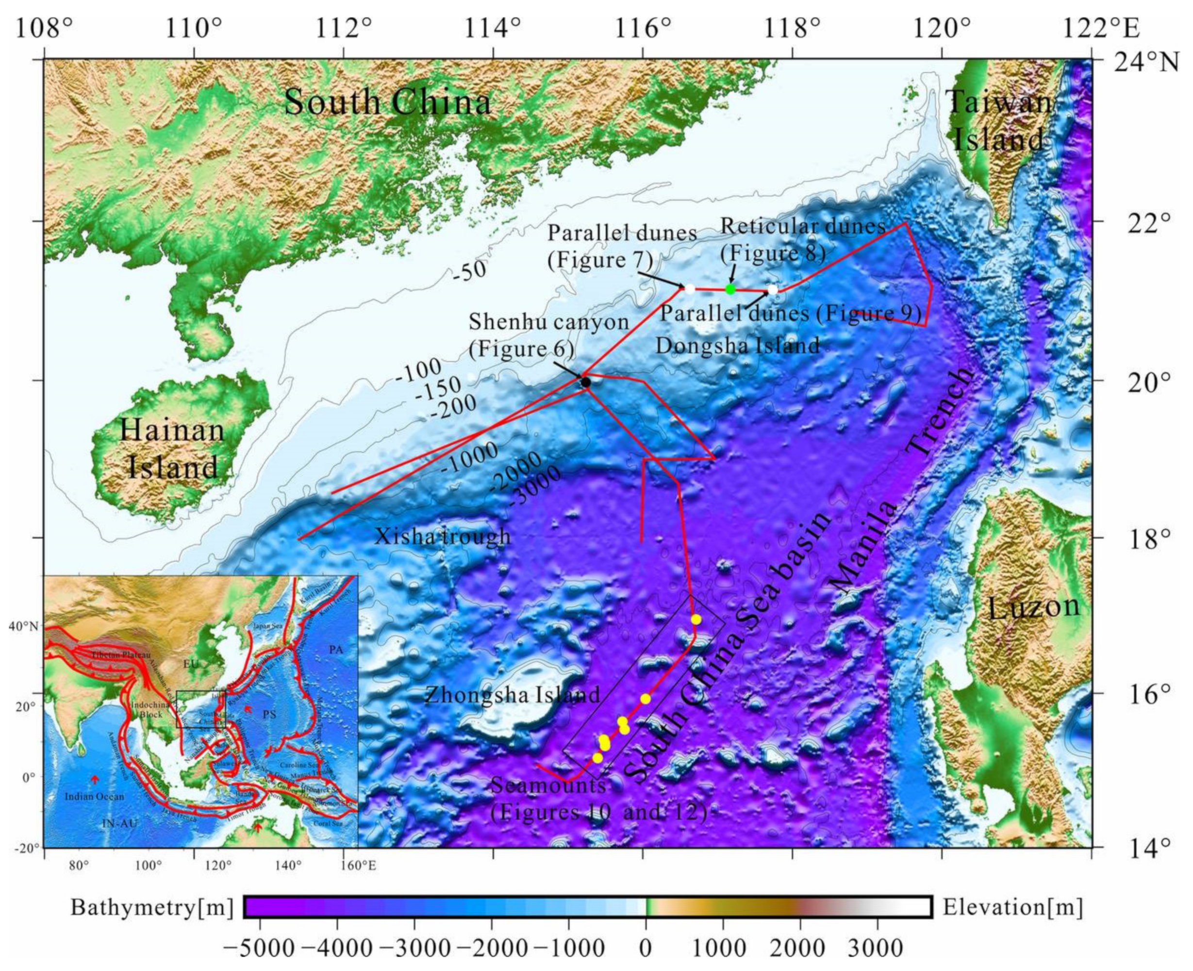
:1. Introduction
2. Bathymetry Data Acquisition and Processing
2.1. Multi-Beam Bathymetry Acquisition System
2.2. Bathymetry Data Processing
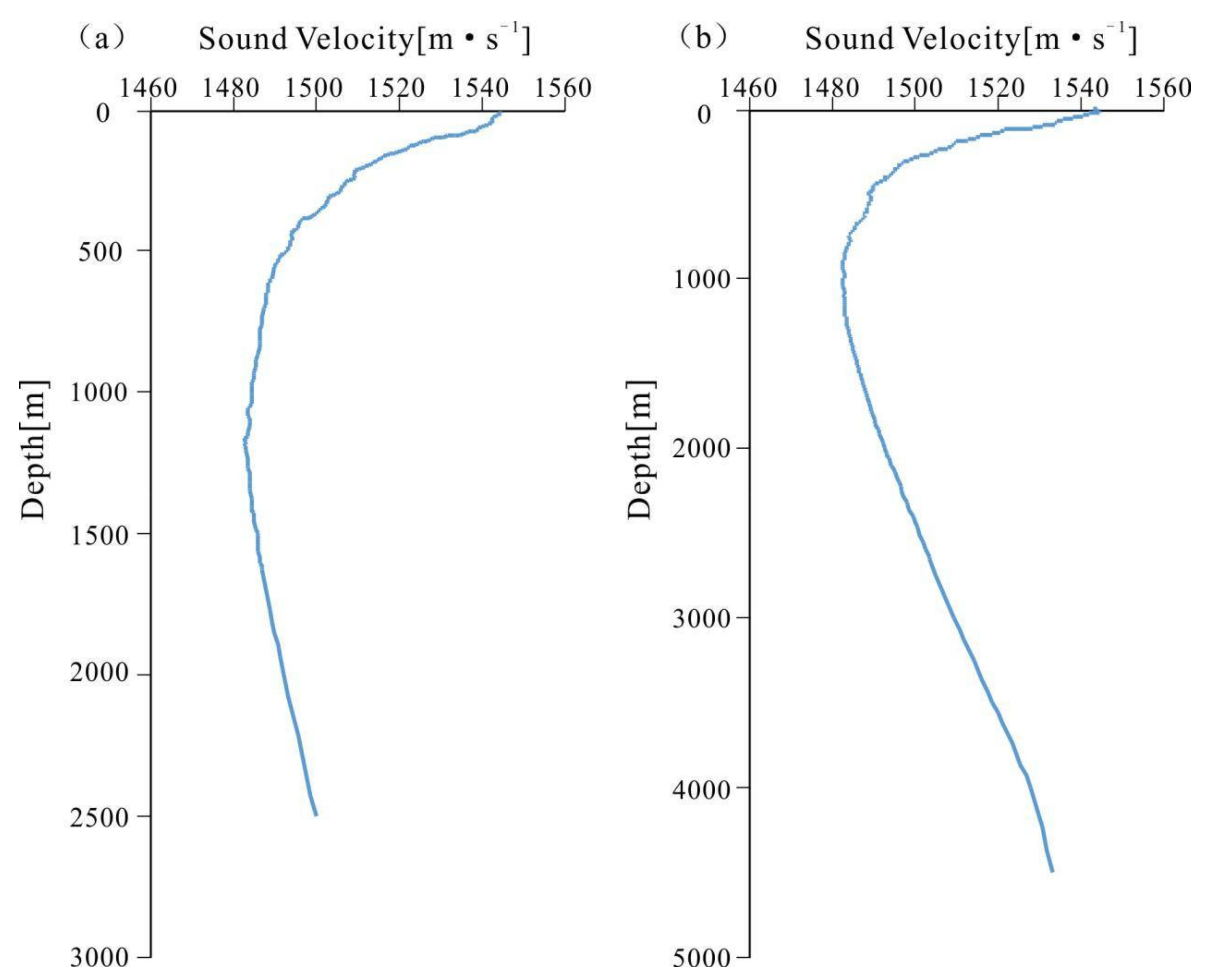
2.2.1. Sound Velocity Correction
2.2.2. Bathymetry Data Editing and Filtering
2.2.3. Bathymetry Data Interpolation
3. Bathymetry Data Anomaly Correction
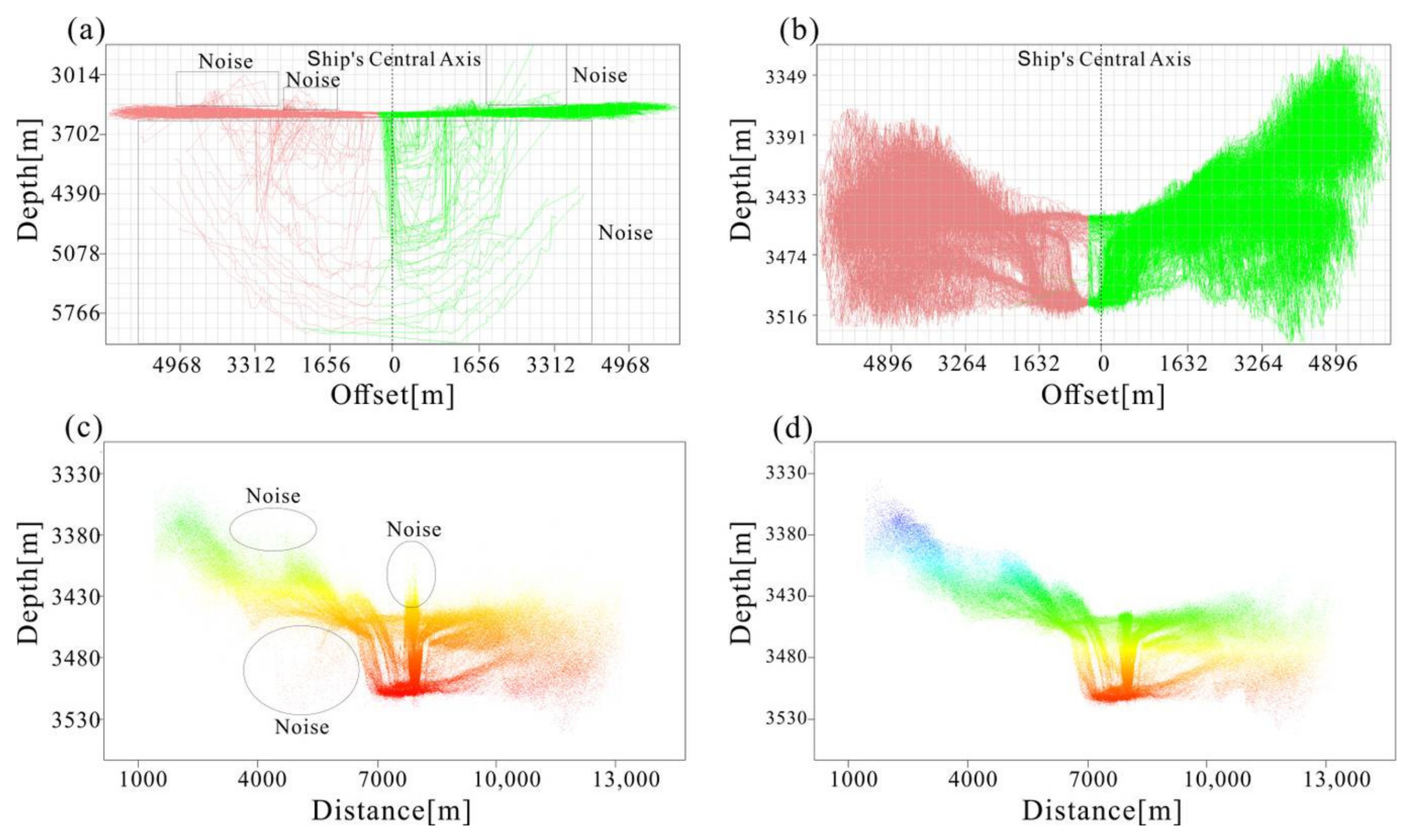
3.1. Anomaly Correction in the Central Beam Area
3.2. Anomaly Correction in the Edge-Beam Area
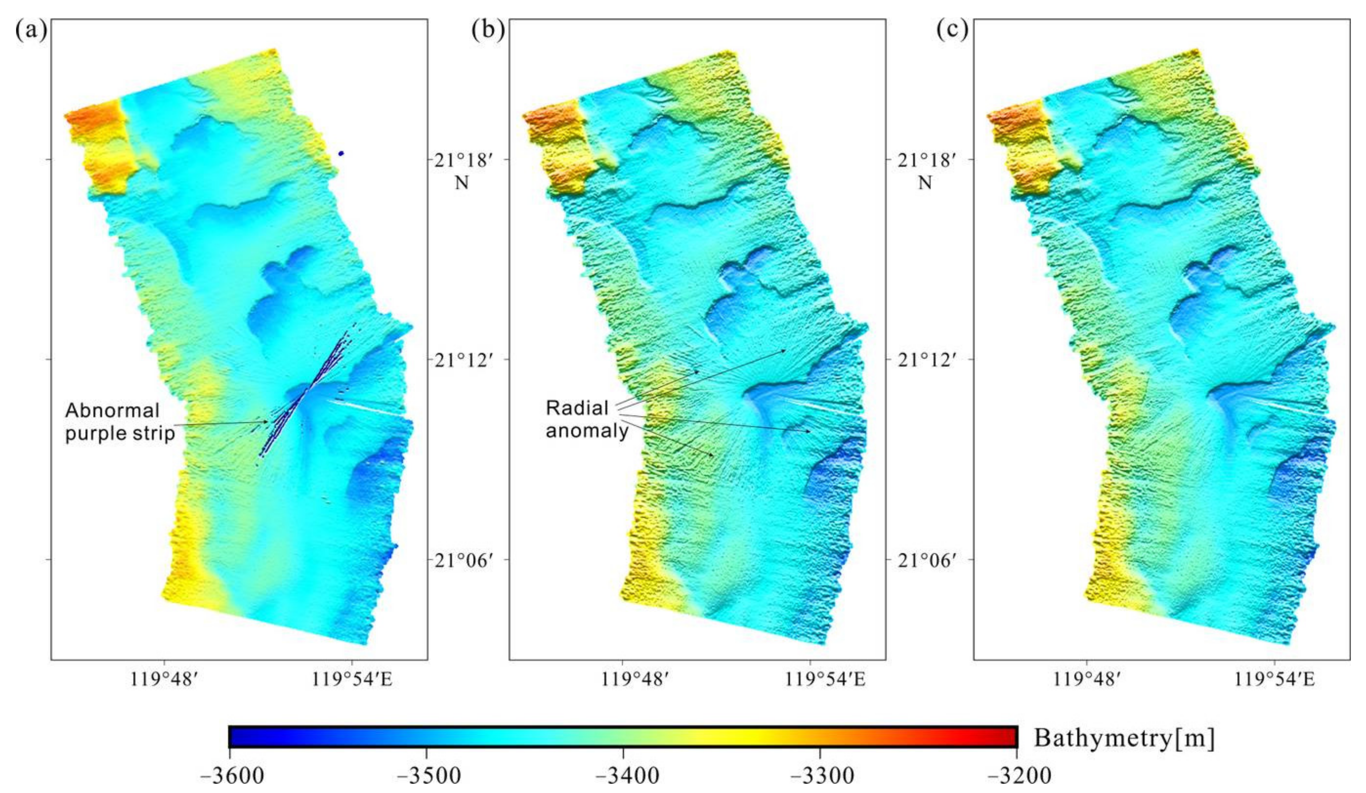
3.3. Correction of Radial Anomalies
4. Results and Discussion
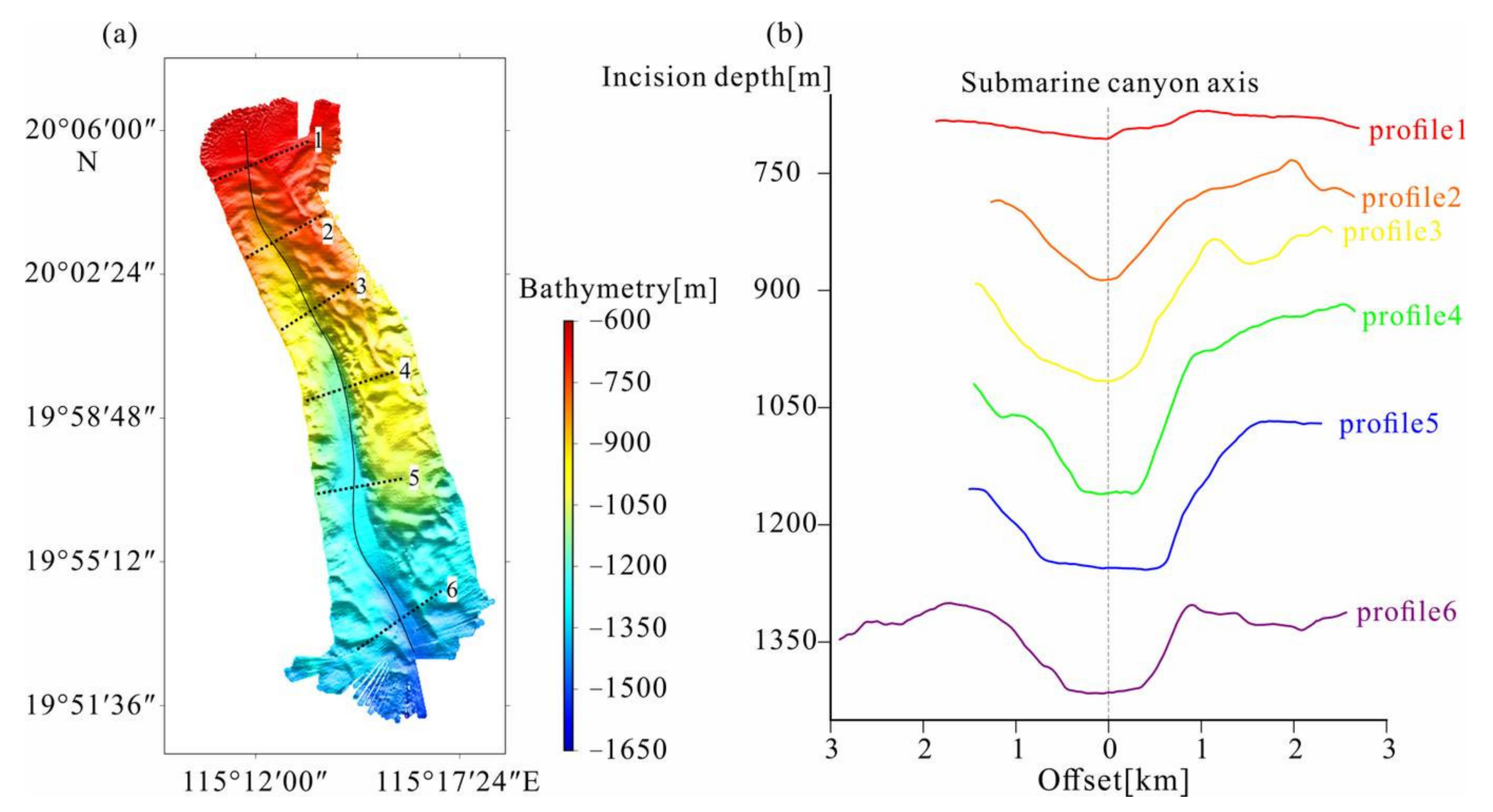
4.1. Geometry and Origins of Submarine Canyons
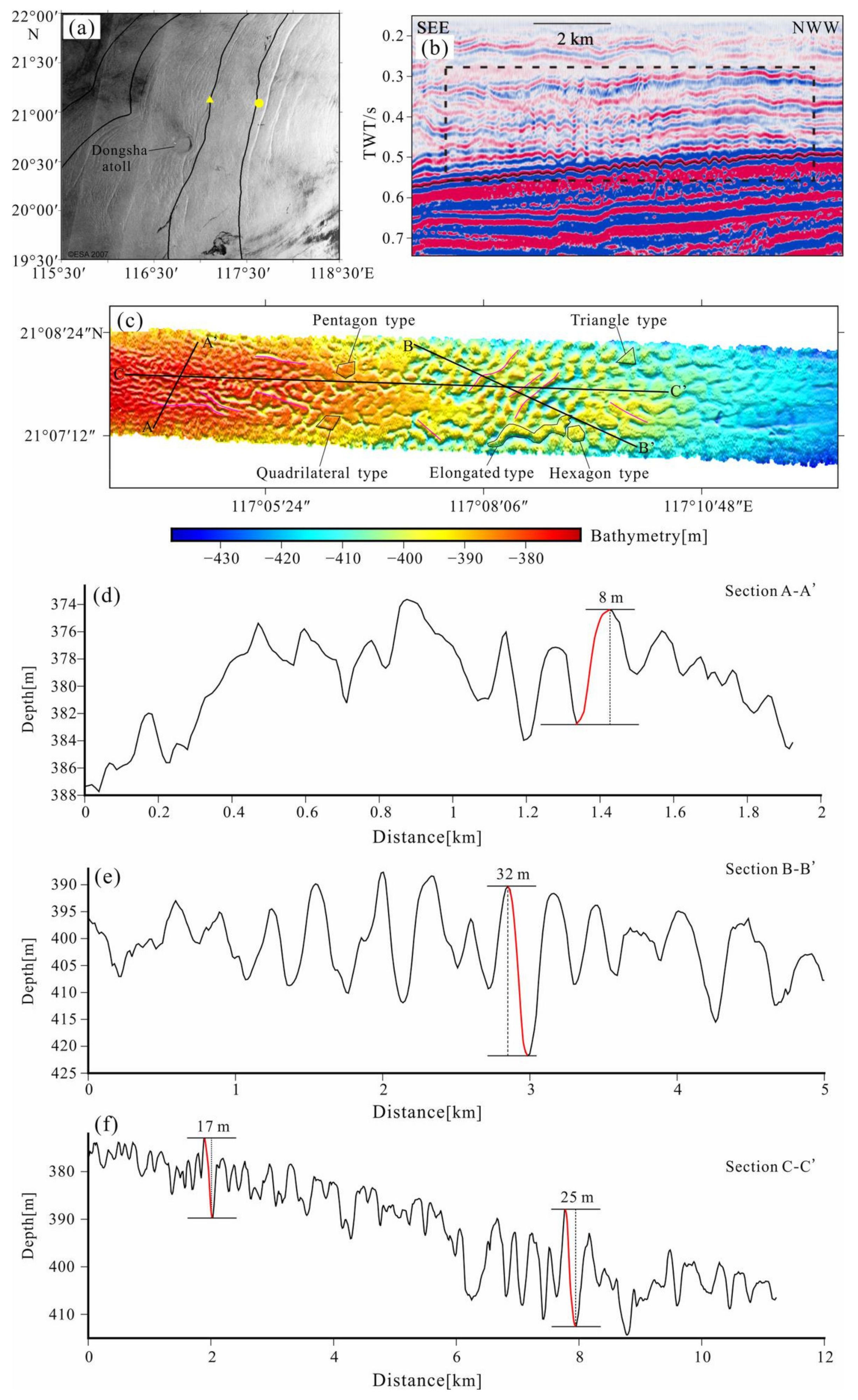
4.2. Geometry and Origins of Submarine Reticular Dunes
4.3. Geometry and Origins of Submarine Parallel Dunes
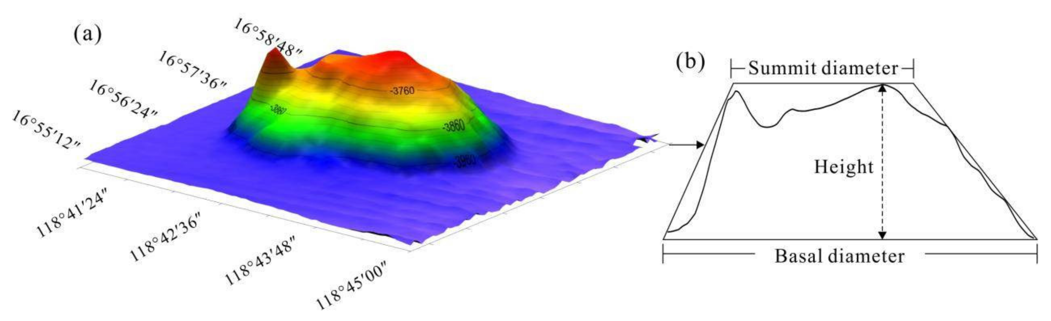
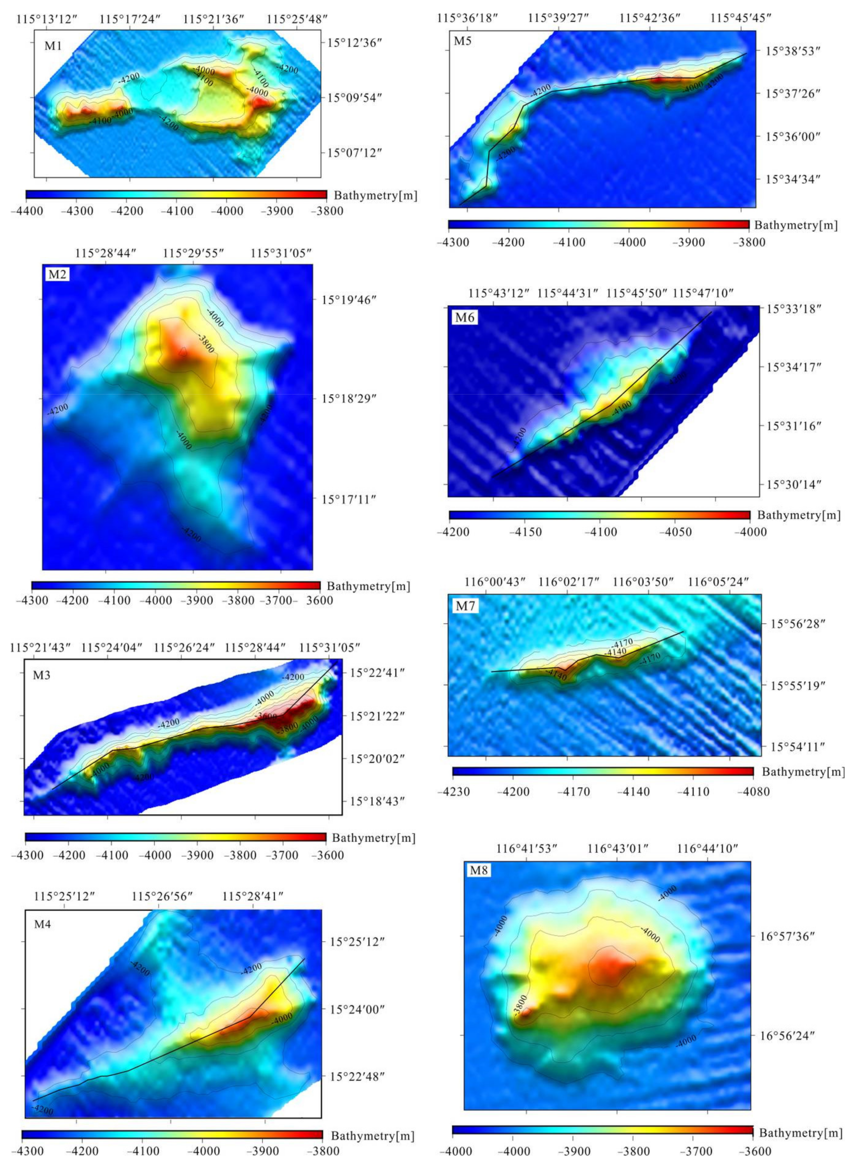
4.4. Geometry and Origins of Seamounts
5. Conclusions
Author Contributions
Funding
Institutional Review Board Statement
Informed Consent Statement
Data Availability Statement
Acknowledgments
Conflicts of Interest
References
- Cervenka, P. Characterization and observation of the seafloor with a new multi-beam front-scan sonar system. In Proceedings of the Third European Marine Science and Technology Conference, Lisbon, Portugal, 23–27 May 1998; Volume 3, pp. 1287–1297. [Google Scholar]
- Zhao, J.H.; Liu, J.N. Problems on the conformity to the real sounding points from the multi-beam sounding system. Hydrogr. Surv. Charting 2003, 1, 6–12. [Google Scholar] [CrossRef]
- Pautot, G.; Rangin, C.; Briais, A.; Tapponnier, P.; Beuzart, P.; Lericolais, G.; Mathieu, X.; Wu, J.; Han, S.; Li, H.; et al. Spreading direction in the central South China Sea. Nature 1986, 321, 150–154. [Google Scholar] [CrossRef]
- Zhang, H.D.; Zhu, B.D.; Guan, Y.X.; Yang, S.X. Topographic features of the seamounts in the central basin of the South China Sea: Based on multi-beam bathymetric data. Mar. Geol. Quat. Geol. 2017, 37, 149–157. [Google Scholar] [CrossRef]
- Zhang, H.D.; Zhu, B.D.; Huang, W.X.; Liu, L.Q.; Chen, H.J. Distribution of guyots on the northwestern slope of South China Sea and their topographic features. Mar. Geol. Front. 2017, 33, 11–17. [Google Scholar] [CrossRef]
- Smoot, N.C. Guyots of the Dutton ridge at the Bonon/Mariana trench juncture as shown by multi-beam surveys. J. Geol. 1983, 91, 211–220. [Google Scholar] [CrossRef]
- Smoot, N.C. Observations on Gulf of Alaska seamount chains by multi-beam sonar. Tectonophysics 1985, 115, 235–246. [Google Scholar] [CrossRef]
- Gardner, J.V.; Hughes, C.J.E.; Mayer, L.A. Bathymetry and Acoustic Backscatter of the Mid and Outer Continental Shelf, Head of De Soto Canyon, Northeastern Gulf of Mexico; US Geological Survey Open-File Report; US Department of the Interior: Washington, DC, USA, 2002; Volume 2, p. 396.
- Wiles, E.; Green, A.; Watkeys, M.; Botes, R.; Jokat, W. Submarine canyons of NW Madagascar: A first geomorphological insight. Deep. Sea Res. Part II Top. Stud. Oceanogr. 2019, 161, 5–15. [Google Scholar] [CrossRef]
- Gardner, J.V.; Dartnell, P.; Mayer, L.A.; Clarke, J.E.H. Geomorphology, acoustic backscatter, and processes in Santa Monica Bay from multibeam mapping. Mar. Environ. Res. 2003, 56, 15–46. [Google Scholar] [CrossRef]
- Barnard, P.L.; Hanes, D.M.; Lescinski, J.; Elias, E. Monitoring and modeling nearshore dredge disposal for indirect beach nourishment, Ocean Beach, San Francisco. Coast. Eng. 2007, 5, 4192–4204. [Google Scholar] [CrossRef]
- Xu, J.P.; Wong, F.L.; Kvitek, R.; Smith, D.P.; Paulld, C.K. Sandwave migration in Monterey submarine canyon, central California. Mar. Geol. 2008, 248, 193–212. [Google Scholar] [CrossRef]
- Chen, Y.W.; Song, H.B.; Guan, Y.X.; Geng, M.H.; Liu, S.X. Discovery of the reticular sand dunes in the Dongsha region of South China Sea and their genesis. Chin. J. Geophys. 2018, 61, 1013–1024. [Google Scholar] [CrossRef]
- Bai, Y.; Song, H.B.; Guan, Y.X.; Chen, J.X.; Liu, B.R. Structural characteristics and genesis of pockmarks in the northwest of the South China Sea derived from reflective seismic and multibeam data. Chin. J. Geophys. 2014, 57, 2208–2222. [Google Scholar] [CrossRef]
- Dandapath, S.; Chakraborty, B.; Maslov, N.; Karisiddaiah, S.M.; Ghosh, D.; Fernandes, W.; Menezes, A. Characterization of seafloor pockmark seepage of hydrocarbons employing fractal: A case study from the western continental margin of India. Mar. Pet. Geol. 2012, 29, 115–128. [Google Scholar] [CrossRef]
- Kelley, J.T.; Barber, D.C.; Belknap, D.F.; FitzGerald, D.M.; Heteren, S.V.; Dickson, S.M. Sand budgets at geological, historical and contemporary time scales for a developed beach system, Saco Bay, Maine, USA. Mar. Geol. 2005, 214, 117–142. [Google Scholar] [CrossRef]
- Tapponnier, P.; Molnar, P. Slip-line field theory and large-scale continental tectonics. Nature 1976, 264, 319–324. [Google Scholar] [CrossRef]
- Taylor, B.; Hayes, D.E. Origin and History of the South China Sea Basin. In The Tectonic and Geologic Evolution of Southeast Asian Seas and Islands: Part 2; American Geophysical Union: Washington, DC, USA, 1983; Volume 27, pp. 23–56. [Google Scholar] [CrossRef]
- Yao, B.C.; Liu, Z.H. Sedimentary basins and petroleum resources in Nansha offshore area, South China Sea. China Offshore Oil Gas 2006, 3, 150–160. [Google Scholar] [CrossRef]
- Maruyama, S.; Santosh, M.; Zhao, D. Superplume, supercontinent, and post-perovskite: Mantle dynamics and anti-plate tectonics on the core-mantle boundary. Gondwana Res. 2007, 11, 7–37. [Google Scholar] [CrossRef]
- Li, C.F.; Zhou, Z.; Li, J.; Hao, H.J.; Geng, J.H. Structures of the northeasternmost South China Sea continental margin and ocean basin: Geophysical constraints and tectonic implications. Mar. Geophys. Res. 2007, 28, 59–79. [Google Scholar] [CrossRef]
- Li, C.F.; Zhou, Z.; Li, J.; Chen, B.; Geng, J. Magnetic zoning and seismic structure of the South China Sea ocean basin. Mar. Geophys. Res. 2008, 29, 223–238. [Google Scholar] [CrossRef]
- Ben-Avraham, Z.; Uyeda, S. The evolution of the China Basin and the Mesozoic paleogeography of Borneo. Earth Planet. Sci. Lett. 1973, 18, 365–376. [Google Scholar] [CrossRef]
- Yao, B.C. The sea floor spreading in the SW Subbasin of South China Sea and it’ s tectonic significance. Geol. Res. S. China Sea 1997, 9, 20–36. [Google Scholar]
- Yao, B.C. Arguments on the sea floor spreading ages of South China Sea basin. Geol. Res. S. China Sea 1998, 10, 23–33. [Google Scholar]
- Yang, J.Y.; Zhang, X.H.; Wang, X.T. Using Gravitational and Magnetic Calculation to Interpret the Earth’ s Crust Characteristics of the Middle Part of the South China Sea. Mar. Geol. Quat. Geol. 2001, 21, 45–50. [Google Scholar] [CrossRef]
- Barckhausen, U.; Engels, M.; Franke, D.; Ladage, S.; Pubellier, M. Evolution of the South China Sea: Revised ages for breakup and seafloor spreading. Mar. Pet. Geol. 2014, 58, 599–611. [Google Scholar] [CrossRef]
- Liu, Z.C.; Chen, Y.L.; Ding, J.S.; Zhang, W.H.; Wu, Y.T.; Guo, F.B. Study on zoned characteristics and formation cause of the east china sea submarine topography. Adv. Mar. Sci. 2003, 2, 160–173. [Google Scholar] [CrossRef]
- Lee, J.T. Topography, Echo Characters (3.5 khz) and Tectonics of the Kaoping Slope off Southwesten Taiwan Coast; National Taiwan University: Taipei, Taiwan, 1992. [Google Scholar]
- Chen, H.J.; Cai, G.Q.; Luo, W.D.; Wu, J.Q.; Huang, L.; Li, L.Q. Features of canyon morphology and their origin in the shenhu area, northern slope of the South China sea. Mar. Geol. Quat. Geol. 2012, 32, 19–26. [Google Scholar] [CrossRef]
- Ding, W.W.; Li, J.B.; Li, J. Morphotectonics and evolutionary controls on the Pearl River Canyon system, South China Sea. Mar. Geophys. Res. 2013, 34, 221–238. [Google Scholar] [CrossRef] [Green Version]
- Han, X.; Li, J.; Chu, F.; Li, J.; Yang, F.L. Geomorphology and tectonic interpretation of Zhujiang Submarine Canyon, in the northern South China Sea. In Proceedings of the OCEANS’10 IEEE, Sydney, Australia, 24–27 May 2010; IEEE: Sydney, Australia, 2010; pp. 1–4. [Google Scholar] [CrossRef]
- Chuang, P.; Yang, T.F.; Lin, S.; Lee, H.E.; Lan, T.F.; Hong, W.; Sun, C.; Chen, Y.; Chen, J.; Wang, Y. Gas geochemistry study in gas hydrate potential area offshore SW Taiwan. In Proceedings of the AGU Fall Meeting Abstracts, OS33B-1690, San Francisco, CA, USA, 11–15 December 2006. [Google Scholar]
- Li, S.J.; Chu, F.Y.; Fang, Y.X.; Wu, Z.Y.; Ni, Y.G. Associated interpretation of sub-bottom and single-channel seismic profiles from slope of Shenhu Area in the northern South China Sea-characteristics of gas hydrate sediment. J. Trop. Oceanogr. 2010, 29, 56–62. [Google Scholar] [CrossRef]
- Wang, X.J.; Wu, S.G.; Dong, D.D.; Guo, Y.Q.; Deborah, H. Control of mass transport deposits over the occurrence of gas hydrate in qiongdongnan basin. Mar. Geol. Quat. Geol. 2011, 31, 109–118. [Google Scholar] [CrossRef]
- Peng, X.C.; Wu, L.S.; Cui, Z.G.; Liu, S.X.; Wang, Y.T. A stability analysis of seabed sand waves in waters north of Dongsha Islands of South China Sea. J. Trop. Oceanogr. 2006, 3, 21–27. [Google Scholar] [CrossRef]
- Du, X.Q.; Li, Y.; Gao, S. Characteristics of the large-scale sand waves, tidal flow structure and bedload transport over the Taiwan Bank in southern China. Acta Oceanol. Sin. 2008, 5, 124–136. [Google Scholar] [CrossRef]
- Zeng, C.K.; Wang, X.B. Distribution and genesis of the seamounts and hills in the South China Sea. Donghai Mar. Sci. 1987, 5, 1–9. [Google Scholar]
- Wang, Y.B.; Wu, Z.Y.; Shang, J.H.; Yin, S.R.; Zhao, D.N.; Zhou, J.Q. Morphologic characteristics and controlling factors of the northeastern South China Sea canyon group. Haiyang Xuebao 2020, 42, 62–74. [Google Scholar]
- GEBCO Bathymetric Compilation Group 2021. The GEBCO_2021 Grid-a continuous terrain model of the global oceans and land. NERC EDS British Oceanographic Data Centre NOC. 2021. Available online: https://www.gebco.net/data_and_products/gridded_bathymetry_data/gebco_2021/documents/GEBCO_2021_Grid.pdf (accessed on 11 August 2020).
- Universal System. CARIS HIPS & SIPS User Guide. 2013. Available online: http://www.teledynecaris.com/en/search/?Search=CARIS+HIPS+%26+SIPS+User+Guide (accessed on 8 August 2020).
- Wessel, P.; Smith, W.H.F. New, improved version of Generic Mapping Tools released. Eos Trans. Am. Geophys. Union 1998, 79, 579. [Google Scholar] [CrossRef]
- Maritime, K. Kongsberg EM122 Multimate Echo Sounder Maintenance Manual. 2009. Available online: https://www.kongsberg.com/search/?searchTerm=em122 (accessed on 7 August 2020).
- Farr, H.K. Multibeam bathymetric sonar: Sea beam and hydro chart. Mar. Geod. 1980, 4, 77–93. [Google Scholar] [CrossRef]
- Hellequin, L.; Boucher, J.M.; Lurton, X. Processing of high-frequency multibeam echo sounder data for seafloor characterization. IEEE J. Ocean. Eng. 2003, 28, 78–89. [Google Scholar] [CrossRef] [Green Version]
- Yang, L.; Taxt, T. Multibeam sonar bottom detection using multiple subarrays. In Proceedings of the Oceans ’97. MTS/IEEE Conference Proceedings, Halifax, NS, Canada, 6–9 October 1997; Volume 2, pp. 932–938. [Google Scholar] [CrossRef]
- William, J.; Capell, S. Determination of sound velocity profile errors using multibeam data. In Proceedings of the Oceans ’99/MTS/IEEE. Riding the Crest into the 21st Century, Seattle, WA, USA, 13–16 September 1999; Volume 3, pp. 1144–1148. [Google Scholar] [CrossRef]
- Vande, W.T. Mapping with multibean data: Are there ideal model settings? 2002. Available online: https://agris.fao.org/agris-search/search.do?recordID=AV20120152135 (accessed on 10 August 2020).
- Shaw, S.; Arnold, J. Automated error detection in multibeam bathymetry data. In Proceedings of the OCEANS’93, Victoria, BC, Canada, 18–21 October 1993; IEEE: Victoria, BC, Canada, 1993; Volume 2, pp. II/89–II/94. [Google Scholar] [CrossRef]
- Yang, F.; Zhao, C.; Zhang, K.; Feng, C.K.; Ma, Y. Calibrating nadir striped artifacts in a multibeam backscatter image using the equal mean-variance fitting model. J. Appl. Remote Sens. 2017, 11, 035020. [Google Scholar] [CrossRef]
- Wu, Z.Y.; Jin, X.L.; Zheng, Y.L.; Li, J.B.; Yu, P. Integrated error correction of multi-beam marginal sounding beam. Acta Oceanol. Sin. 2005, 4, 88–94. [Google Scholar] [CrossRef]
- Yang, F.L.; Li, J.B.; Wu, Z.Y.; Jin, X.L.; Chu, F.Y. The Methods of High Quality Post-Processing for Shallow Multibeam Data. Acta Geod. Cartogr. Sin. 2008, 37, 444–457. [Google Scholar]
- Daly, R.A. Origin of submarine canyons. Am. J. Sci. 1936, 5, 401–420. [Google Scholar] [CrossRef]
- Shepard, F.P. Submarine canyons. Earth-Sci. Rev. 1972, 8, 1–12. [Google Scholar] [CrossRef]
- Normark, W.R.; Carlson, P.R.; Chan, M.A. Giant submarine canyons: Is size any clue to their importance in the rock record? Spec. Pap. Geol. Soc. Am. 2003, 175–190. [Google Scholar] [CrossRef]
- Wang, C.S.; Zhu, J.J.; Zhao, D.D.; Yang, G.M.; Xiong, Z.X.; Zhang, S.S.; Li, S.Z.; JIA, Y.G. Origin and evolution of submarine canyons. Mar. Geol. Front. 2021, 37, 1–15. [Google Scholar] [CrossRef]
- Harris, P.T.; Whiteway, T. Global distribution of large submarine canyons: Geomorphic differences between active and passive continental margins. Mar. Geol. 2011, 285, 69–86. [Google Scholar] [CrossRef]
- Greene, H.G.; Hicks, K.R. Ascension-Monterey Canyon system: History and development. In Geology and Tectonics of the Central California Coast Region: San Francisco to Monterey; Garrison, R.E., Ed.; Pacific Section AAPG: College Station, CA, USA, 1990; pp. 229–249. [Google Scholar]
- Inman, D.L.; Jenkins, S.A. Climate change and the episodicity of sediment flux of small California rivers. J. Geol. 1999, 107, 251–270. [Google Scholar] [CrossRef] [Green Version]
- Farnsworth, K.L.; Warrick, J.A. Sources, Dispersal, and Fate of Fine Sediment Supplied to Coastal California; US Geological Survey: Reston, VA, USA, 2007. [Google Scholar] [CrossRef]
- Maier, K.L.; Johnson, S.Y.; Hart, P. Controls on submarine canyon head evolution: Monterey Canyon, offshore central California. Mar. Geol. 2018, 404, 24–40. [Google Scholar] [CrossRef]
- Yu, H.S.; Huang, C.S.; Ku, J.W. Morphology and possible origin of the Kaoping submarine canyon head of southwest Taiwan. Acta Oceanogr. Taiwanic 1990, 27, 40–50. [Google Scholar]
- Chiang, C.S.; Yu, H.S. Morphotectonics and incision of the Kaoping submarine canyon, SW Taiwan orogenic wedge. Geomorphology 2006, 80, 199–213. [Google Scholar] [CrossRef]
- Yu, H.S.; Huang, Z.Y. Morphotectonics and sedimentation in convergent margin basins: An example from juxtaposed marginal sea basin and foreland basin, Northern South China Sea. Tectonophysics 2009, 466, 241–254. [Google Scholar] [CrossRef]
- Yu, H.S.; Chang, E.T.Y. Links among slope morphology, canyon types and tectonics on passive and active margins in the northernmost South China Sea. J. Earth Sci. 2009, 20, 77–84. [Google Scholar] [CrossRef]
- Chiang, C.S.; Yu, H.S. Sedimentary erosive processes and sediment dispersal in Kaoping submarine canyon. Sci. China Earth Sci. 2011, 54, 259–271. [Google Scholar] [CrossRef]
- Pang, X.; Shen, J.; Yuan, L.Z.; He, M.; Shu, Y. Petroleum prospect in deep-water fan system of the Pearl River in the South China Sea. Acta Pet. Sin. 2006, 3, 11–21. [Google Scholar] [CrossRef]
- Xu, M.Q.; Huang, Y.P.; Shi, W.Y.; Chen, M. Study on the Clastic Minerals of the Adjacent Sea Area of Dongsha Archipelago in the South China Sea. J. Xiamen Univ. 1994, 3, 380–385. [Google Scholar]
- Li, L.; Chen, Z.; Liu, J.G.; Chen, H.; Yan, W.; Zhong, Y. Distribution of surface sediment types and sedimentary environment divisions in the northern South China Sea. J. Trop. Oceanogr. 2014, 33, 54–61. [Google Scholar] [CrossRef]
- Ashley, G.M. Classification of large-scale subaqueous bedforms; a new look at an old problem. J. Sediment. Res. 1990, 60, 160–172. [Google Scholar] [CrossRef]
- Allen, J.R.L. Sedimentary Structures: Their Character and Physical Basis; Elsevier: Amsterdam, The Netherlands, 1982. [Google Scholar]
- Jackson, C.R. An empirical model for estimating the geographic location of nonlinear internal solitary waves. J. Atmos. Ocean. Technol. 2009, 26, 2243–2255. [Google Scholar] [CrossRef]
- Guo, C.; Chen, X. A review of internal solitary wave dynamics in the northern South China Sea. Prog. Oceanogr. 2014, 121, 7–23. [Google Scholar] [CrossRef]
- Zhao, W.; Huang, X.; Tian, J. A new method to estimate phase speed and vertical velocity of internal solitary waves in the South China Sea. J. Oceanogr. 2012, 68, 761–769. [Google Scholar] [CrossRef]
- Fu, K.H.; Wang, Y.H.; Laurent, L.S.; Simmons, H.; Wang, D.P. Shoaling of large-amplitude nonlinear internal waves at Dongsha Atoll in the northern South China Sea. Cont. Shelf Res. 2012, 37, 1–7. [Google Scholar] [CrossRef] [Green Version]
- Lü, H.; He, Y.; Shen, H.; Cui, L.M.; Dou, C.E. The propagating speed of internal solitary waves investigated by X-band radar near Dongsha Island. In Proceedings of the 2010 IEEE International Geoscience and Remote Sensing Symposium, Honolulu, HI, USA, 25–30 July 2010; IEEE: Honolulu, HI, USA, 2010; pp. 4705–4708. [Google Scholar] [CrossRef]
- Geng, M.H.; Song, H.B.; Guan, Y.X.; Bai, Y.; Liu, S.X.; Chen, Y.W. The distribution and characteristics of very large subaqueous sand dunes in the Dongsha region of the northern South China Sea. Chin. J. Geophys. 2017, 60, 628–638. [Google Scholar] [CrossRef]
- Wang, S.Y.; Gu, Y.; Guo, C.Z. Sediment Mathematical Model to Estuarine Engineering; China Ocean Press: Beijing, China, 1990. [Google Scholar]
- Reeder, D.B.; Ma, B.B.; Yang, Y.J. Very large subaqueous sand dunes on the upper continental slope in the South China Sea generated by episodic, shoaling deep-water internal solitary waves. Mar. Geol. 2011, 279, 12–18. [Google Scholar] [CrossRef]
- Belde, J.; Back, S.; Reuning, L. Three-dimensional seismic analysis of sediment waves and related geomorphological features on a carbonate shelf exposed to large amplitude internal waves, Browse Basin region, Australia. Sedimentology 2015, 62, 87–109. [Google Scholar] [CrossRef]
- Landeghem, K.; Wheeler, A.J.; Mitchell, N.C.; Sutton, G. Variations in sediment wave dimensions across the tidally dominated Irish Sea, NW Europe. Mar. Geol. 2009, 263, 108–119. [Google Scholar] [CrossRef]
- Yu, W.; Wu, Z.Y.; Zhou, J.Q.; Zhao, D.N. Meticulous characteristics, classification and distribution of seabed sand wave on the Taiwan bank. Acta Oceanol. Sin. 2015, 37, 11–25. [Google Scholar] [CrossRef]
- Feng, W.K.; Bao, C.W. Topographic and geomorphological characteristics of South China Sea. Mar. Geol. Res. 1982, 4, 80–93. [Google Scholar] [CrossRef]
- Xia, J.Q.; Tan, G.M. Numerical Simulation of sediment deposition and horizontal axis circulation flow in lateral trenches. J. Hydraul. Eng. 1999, 8, 51–56. [Google Scholar] [CrossRef]
- Menard, H.W. Marine Geology of the Pacific; McGraw-Hill: New York, NY, USA, 1964. [Google Scholar]
- Magee, C.; Hunt-Stewart, E.; Jackson, C.A.L. Volcano growth mechanisms and the role of sub-volcanic intrusions: Insights from 2D seismic reflection data. Earth Planet. Sci. Lett. 2013, 373, 41–53. [Google Scholar] [CrossRef]
- Briais, A.; Patriat, P.; Tapponnier, P. Updated interpretation of magnetic anomalies and seafloor spreading stages in the South China Sea: Implications for the Tertiary tectonics of Southeast Asia. J. Geophys. Res. Atmos. 1993, 98, 6299–6328. [Google Scholar] [CrossRef] [Green Version]
- Li, C.-F.; Xu, X.; Lin, J.; Sun, Z.; Zhu, J.; Yao, Y.; Zhao, X.; Liu, Q.; Kulhanek, D.K.; Wang, J.; et al. Ages and magnetic structures of the South China Sea constrained by deep tow magnetic surveys and IODP Expedition 349. Geochem. Geophys. Geosyst. 2014, 15, 4958–4983. [Google Scholar] [CrossRef]
- Pautot, G.; Rangin, C. Subduction of the South China Sea axial ridge below Luzon (Philippines). Earth Planet. Sci. Lett. 1989, 92, 57–69. [Google Scholar] [CrossRef]


| EM122 (the R/V “Dongfanghong 3”) | |
|---|---|
| Basic Principle | Beam Forming |
| Main operational frequency | 12 kHz |
| Depth ranges from transducers | 20–11,000 m |
| Beam widths | 0.5 × 1°, 1 × 1°, 1 × 2°, 2 × 2°, or 2 × 4° |
| Coverage sector | 150° |
| Maximum strip width | Six times the water depth |
| Maximum coverage width | 30 km |
| Beam number | 288 |
| Range sampling rate | 3 kHz |
| Sounding resolution | 10–40 cm |
| Sounding accuracy | 0.3% water depth |
| Beam spacing | Equidistant, equiangle or in between |
| Maximum operating speed | 16 Knots |
| Geomorphology Features | Length [m] | Width [m] | Height [m] | Filter Methods |
|---|---|---|---|---|
| Shenhu canyon | ~21,000 | 2000–3000 | 90–230 | Swath and surface filtering |
| Reticular dunes | 50–600 | 50–300 | 8–32 | Surface filtering |
| Parallel dunes | 100–1000 | 50–300 | 2–20 | Surface filtering |
| Seamounts | 8200–23,000 | 2700–11,100 | 111–778 | Swath and surface filtering |
| Number | Lat/Lon | Summit Depth [m] | Basal Depth [m] | Height [m] | Summit Radius [km] | Basal Radius [km] | Area [km2] | Ratios | Flatness | Type | Trend |
|---|---|---|---|---|---|---|---|---|---|---|---|
| M1 | 115°15′10″ E 15°09′12″ N | 3854 | 4283 | 429 | 2 | 3.7 | 119.8 | 0.12 | 0.54 | Irregular | — |
| M2 | 115°29′48″ E 15°19′08″ N | 3693 | 4236 | 543 | 0.9 | 4.1 | 19.6 | 0.13 | 0.22 | Irregular | — |
| M3 | 115°29′38″ E 15°21′20″ N | 3485 | 4263 | 778 | 1.8 | 5.2 | 39.7 | 0.15 | 0.35 | Linear | NEE |
| M4 | 115°28′27″ E 15°23′42″ N | 3873 | 4238 | 365 | 1.1 | 3.49 | 24.5 | 0.10 | 0.32 | Linear | NEE |
| M5 | 115°42′52″ E 15°37′58″ N | 3813 | 4245 | 432 | 1.9 | 5.9 | 29.8 | 0.07 | 0.32 | Linear | NE |
| M6 | 115°44′35″ E 15°31′06″ N | 4048 | 4250 | 202 | 0.9 | 2.5 | 10.9 | 0.22 | 0.36 | Linear | NE |
| M7 | 116°22′23″ E 15°55′35″ N | 4104 | 4198 | 94 | 0.5 | 1.9 | 8.5 | 0.05 | 0.26 | Linear | NEE |
| M8 | 116°42′53″ E 16°57′09″ N | 3666 | 4041 | 375 | 1.2 | 2.5 | 19.7 | 0.15 | 0.48 | Conical | — |
Publisher’s Note: MDPI stays neutral with regard to jurisdictional claims in published maps and institutional affiliations. |
© 2021 by the authors. Licensee MDPI, Basel, Switzerland. This article is an open access article distributed under the terms and conditions of the Creative Commons Attribution (CC BY) license (https://creativecommons.org/licenses/by/4.0/).
Share and Cite
Ou, X.; Zhu, J.; Li, S.; Jia, Y.; Jia, Z.; Zhang, S.; Zhang, S.; Chen, R.; Chen, X.; Ding, D.; et al. Submarine Geomorphological Features and Their Origins Analyzed from Multibeam Bathymetry Data in the South China Sea. J. Mar. Sci. Eng. 2021, 9, 1419. https://doi.org/10.3390/jmse9121419
Ou X, Zhu J, Li S, Jia Y, Jia Z, Zhang S, Zhang S, Chen R, Chen X, Ding D, et al. Submarine Geomorphological Features and Their Origins Analyzed from Multibeam Bathymetry Data in the South China Sea. Journal of Marine Science and Engineering. 2021; 9(12):1419. https://doi.org/10.3390/jmse9121419
Chicago/Turabian StyleOu, Xiaolin, Junjiang Zhu, Sanzhong Li, Yonggang Jia, Zhongjia Jia, Shengsheng Zhang, Shaoyu Zhang, Ruixue Chen, Xingquan Chen, Dong Ding, and et al. 2021. "Submarine Geomorphological Features and Their Origins Analyzed from Multibeam Bathymetry Data in the South China Sea" Journal of Marine Science and Engineering 9, no. 12: 1419. https://doi.org/10.3390/jmse9121419