Article

Time Scale for Scour Beneath Pipelines Due to Long-Crested and Short-Crested Nonlinear Random Waves Plus Current

1
Department of Marine Technology, Norwegian University of Science and Technology (NTNU), 7491 Trondheim, Norway
2
Department of Mechanical and Structural Engineering and Materials Science, University of Stavanger, 4036 Stavanger, Norway
*
Author to whom correspondence should be addressed.
J. Mar. Sci. Eng. 2021, 9(2), 114; https://doi.org/10.3390/jmse9020114
Submission received: 3 December 2020 / Revised: 7 January 2021 / Accepted: 14 January 2021 / Published: 22 January 2021
(This article belongs to the Special Issue Wave–Current Interaction in Coastal Areas)

Abstract

:
This article derives the time scale of pipeline scour caused by 2D (long-crested) and 3D (short-crested) nonlinear irregular waves and current for wave-dominant flow. The motivation is to provide a simple engineering tool suitable to use when assessing the time scale of equilibrium pipeline scour for these flow conditions. The method assumes the random wave process to be stationary and narrow banded adopting a distribution of the wave crest height representing 2D and 3D nonlinear irregular waves and a time scale formula for regular waves plus current. The presented results cover a range of random waves plus current flow conditions for which the method is valid. Results for typical field conditions are also presented. A possible application of the outcome of this study is that, e.g., consulting engineers can use it as part of assessing the on-bottom stability of seabed pipelines.

1. Introduction

This article addresses the time scale of pipeline scour due to 2D (long-crested) and 3D (short-crested) nonlinear irregular waves and current with the objective of providing a method suitable to use for the practical engineering assessment of pipeline scour. Pipelines originally placed, e.g., on plane beds, will experience the seabed conditions change, i.e., the bed may be flat or with ripples; they may be partly or fully buried or surrounded by scour holes. These changed conditions are due to the complex flow generated by waves plus current and the interaction with the pipeline and the seabed. Real waves are characterized by three-dimensional stochastic features that should be accounted for.
To the best of our knowledge, no study exists in the open literature on the investigation of the time scale for scour beneath pipelines caused by 2D and 3D nonlinear irregular waves plus current. Previously, Myrhaug et al. [1] provided the time scale for the equilibrium scour depth beneath pipelines exposed to 2D and 3D nonlinear irregular waves. Thus, this work is a continuation by extending the method to cover combined waves and current.
The background and details of pipeline scour are provided by, e.g., Whitehouse [2] as well as Sumer and Fredsøe [3], including literature reviews up to that date. Until now, most studies have focused on experimental and numerical work on the equilibrium scour depth beneath pipelines caused by pure current, pure waves and combined waves and current. Exceptions are the recent works of Larsen et al. [4], Zhang et al. [5] and Zang et al. [6] that all three addressed the time scale of equilibrium pipeline scour for waves plus current. Larsen et al. [4] provided an analytical formula for pipeline scour for regular waves plus current based on numerical simulations. Zhang et al. [5] presented a practical time scale formula for regular waves plus current based on small- and large-scale recirculating flume tests. Zang et al. [6] provided results on the time scale of local scour below a partially buried pipeline under combined waves and currents with oblique incident angle based on large-scale flume tests.
Furthermore, most of the works on pipeline scour have considered current alone, regular waves alone, and combined regular waves and current, except Sumer and Fredsøe [7], who provided results from an experimental investigation on scour beneath pipelines exposed to random waves plus current. Myrhaug and Ong [8] reviewed the authors’ works on 2D irregular wave-induced equilibrium scour around marine structures, also comparing with experimental data for irregular wave-induced scour. Myrhaug and Ong [9] provided an approach for calculating the maximum equilibrium scour depth below pipelines due to 2D and 3D nonlinear irregular waves alone.
The aim here is to present a method for estimating the time scale of pipeline scour beneath pipelines exposed to 2D and 3D nonlinear irregular waves and current that can be used as part of an engineering tool when assessing pipeline scour. Results are obtained adopting the Larsen et al. [4] parameterized time scale formula for pipeline scour valid for regular waves plus current jointly with a stochastic method. The random wave process is assumed to be stationary and narrow banded, and nonlinearity is included using the wave crest height distribution given by Forristall [10] covering 2D and 3D second-order nonlinear irregular waves. The Larsen et al. [4] time scale formula is based on best fit to numerical simulations using a fully coupled hydrodynamic and morphologic numerical model based on incompressible Reynolds-averaged Navier–Stokes equations, including a k-ω turbulence closure and seabed morphology. The Forristall [10] parametric crest height distribution is based on using second-order theory including both sum-frequency and difference-frequency effects performed for 2D and 3D irregular waves.
The article contains an Introduction, followed by Section 2 giving the background for linear waves plus current. Section 3 presents the results of the time scale for nonlinear random waves plus current by first giving the theoretical background (Section 3.1), and then providing the outline of the stochastic method (Section 3.2). Section 4 gives results and discussion by first providing a parameter study (Section 4.1) and then giving an example of calculation (Section 4.2). The summary and conclusions are given in Section 5.

2. Background for Linear Waves Plus Current

From observations, it appears that a certain amount of time is required for an equilibrium scour to develop. This time T, referred to as the time scale of the scour process, is defined by (Sumer and Fredsøe [3])
S t = S ( 1 e x p ( t T ) )
where S is the equilibrium scour depth corresponding to the equilibrium situation, and St is the instantaneous scour depth at time t.
The dimensionless time scale T* is (Sumer and Fredsøe [3])
T * = ( g ( γ 1 ) d 50 3 ) 1 / 2 D 2 T
where g is the acceleration due to gravity, γ = rs/r is the sediment grain density (rs) to fluid density (r) ratio, d50 is the medium grain size diameter, and D is the pipeline diameter.
The dimensionless time scale for the equilibrium scour depth beneath pipelines in regular waves and current is given by the following formula based on best fit to numerical simulations (Larsen et al. [4]):
T * = F ( U c w ) θ w c 5 3
F ( U c w ) = 1 50 + 0.015 [ e 350 ( U c w 0.5 ) 2 + e 25 ( U c w 0.53 ) 2 ]
Here,
U c w = U c U c + U
where Uc is the current velocity, U is the undisturbed linear orbital velocity amplitude near the seabed, and F(Ucw) = 1/50 for both waves alone (Ucw = 0) and current alone (Ucw = 1). Equation (3) is valid for live-bed scour for θwc > θcr, θwc is the undisturbed Shields parameter for combined waves plus current flow, and θcr is the threshold value of motion at a flat bed, i.e., θcr ≈ 0.05. Larsen et al. [4] calculated θwc using an equivalent formula to that given by Soulsby [11] (see Larsen et al. [4] for more details). However, here waves and current for wave-dominant situations will be considered, and thus θwc in Equation (3) is replaced with the undisturbed Shields parameter.
θ = τ w ρ g ( γ 1 ) d 50
Here, τw is the maximum bottom shear stress within a wave cycle under waves taken as
τ w ρ = 1 2 f w U 2
and fw is the friction factor, which here is adopted from Myrhaug et al. [12] valid for waves and current for wave-dominant situations (see Myrhaug et al. [12]).
f w = c ( A z 0 ) d
( c , d ) = ( 18 ,   1 )   for   20 < ˜ A / z 0 < ˜ 200
( c , d ) = ( 1.39 ,   0.52 )   for   200 < ˜ A / z 0 < ˜ 11 , 000
( c , d ) = ( 0.112 ,   0.25 )   for   11 , 000 < ˜ A / z 0
where A = U/ω is the near-bed orbital displacement amplitude, ω = 2π/Tw is the angular wave frequency, Tw is the wave period, and z0 = d50/12 is the bed roughness. Using this friction factor for rough turbulent flow gives the advantage of deriving the stochastic approach analytically. Furthermore, A is given in terms of the linear wave amplitude a by
A = a s i n h   k   h
with h as the water depth, and k as the wave number obtained by the dispersion relationship ω2 = gk tanh kh. For colinear waves and current the dispersion relationship is ω = kUc + (gk tanh kh)0.5 (see, e.g., Soulsby [11]), determining k for known values of ω, Uc and h However, for wave-dominant flow, the effect of Uc on k is small, i.e., k is obtained for Uc = 0. Here, wave-dominant flow is considered for Ucw ≤ 0.5. It should be noted that Equation (4) has its maximum for Ucw = 0.5, i.e., F (Ucw = 0.5) = 0.05.

3. Time Scale for Nonlinear Irregular Waves and Current

3.1. Theoretical Background

The theoretical background is similar to that given in Myrhaug et al. [1] and is summarized here for the sake of completeness.
Nonlinear waves are represented by Stokes second-order waves where the nonlinearity is mainly due to the larger velocity beneath the wave crest (i.e., crest velocity) than beneath the wave trough (i.e., trough velocity). It is likely that the larger crest velocity causes the scour, rather than the average of the crest and trough velocities (i.e., corresponding to the linear wave velocity (Catano-Lopera and Garcia [13])). Consequently, the time scale for single irregular Stokes second-order waves is given by Equations (2)–(5) replacing U with the maximum orbital velocity near the seabed beneath the wave crest, Um.
Consider a fixed location in a sea state containing stationary narrow-band irregular waves in finite water depth h consistent with Stokes second-order regular waves. Then, the dimensionless nonlinear crest height, wc = ηc/arms, and the dimensionless nonlinear maximum horizontal particle velocity at the seabed, U ^ m = Um/Urms, are (Dean and Dalrymple [14])
w c = a ^ + O ( k p a r m s )
U ^ m = a ^ + O ( k p a r m s )
Here, a ^ = a/arms is the dimensionless linear wave amplitude, the wave amplitude a is normalized with the rms (root-mean-square) value arms, and
U r m s = ω p a r m s s i n h   k p   h
The second-order (nonlinear) terms are represented by O (kparms) and proportional to kparms, i.e., a characteristic wave steepness of the sea state. Here, kp is the wave number associated with the spectral peak frequency obtained from the dispersion relationship for linear waves (valid for Stokes second-order waves as well)
ω p 2 = g k p   t a n h   k p   h
Next, the inversion of Equation (13), i.e., a ^ = wc − O (kparms) is substituted in Equation (14) giving U ^ m = wc + O (kparms). Thus, a ^ is replaced with wc in the linear term of Um since the error is of second order. By neglecting terms of O (kparms), the maximum near-bed orbital velocity beneath the wave crest in dimensional form becomes
U m = ω p η c s i n h   k p   h
Furthermore, Am = Ump is the maximum orbital displacement near the seabed beneath the wave crest, and A ^ m = Am/Arms is the dimensionless maximum orbital displacement near the seabed, where
A r m s = a r m s s i n h   k p   h
and
ω p = U m A m = U r m s A r m s
by combining Equations (15) and (17).

3.2. Outline of the Stochastic Method

As in Myrhaug et al. [1], it is assumed that the highest waves are responsible for the scour in the stationary narrow-band sea state considered. Moreover, the sea state is assumed to have lasted long enough to develop the equilibrium scour depth. Here, the considered highest waves are those exceeding the probability 1/n, wc1/n (i.e., 1 − P(wc1/n) = 1/n), where P (wc) is the cumulative distribution function (cdf) of the dimensionless crest height wc adopted from Forristall [10] (see Equation (A1) in Appendix A).
The statistical characteristic considered here is the expected (mean) value of the time scale due to the (1/n)th highest wave crests, i.e.,
E [ T * ( w c ) | w c   >   w c 1 / n ] = n w c 1 / n T * ( w c ) p ( w c ) d w c
where T* (wc) is the dimensionless time scale, and p (wc) = dP (wc)/dwc is the probability density function (pdf) of wc. As in Myrhaug et al. [1], the present method is based on assuming that: (1) the free surface elevation is a stationary narrow-band process with zero expectation; (2) the time scale formula for regular waves provided in the previous section (Equations (3)–(5)) is valid for random waves as well. These assumptions are basically the same as those used by the authors in previous studies on pipeline scour due to random waves and partly justified by comparison with data (Myrhaug and Ong [8]).
In a narrow-band sea state Tw = Tp, where Tp = 2π/ωp = 2πArms/Urms using Equation (19). Taking U = Um, A = Am and substituting this in Equations (3)–(8), and using from Equation (19) that Am/Arms = Um/Urms, Equation (3) can be re-arranged to obtain the time scale for individual narrow-band nonlinear irregular waves as (using that U ^ m = wc by deleting terms of O (kparms) as well as utilizing that θ = θrms wc(2 − d))
T * ( w c ) = θ r m s 5 / 3 F [ U c w ( w c ) ] w c 5 ( 2 d ) / 3
where
U c w ( w c ) = U c U r m s / ( w c + U c U r m s )
θ r m s = 1 2 c ( A r m s z 0 ) d U r m s 2 g ( γ 1 ) d 50
Thus, the mean of the time scale due to the (1/n)th highest wave crests is obtained by substituting Equations (21)–(23) in Equation (20). Using the results in Appendix A gives
w c 1 / n = 8 α ( l n   n ) 1 / β
where α and β are the Weibull parameters given in Equations (A4) and (A5), respectively.
Concerning the Shields parameter, it is not obvious which value is the most relevant to use corresponding to live-bed scour. However, as in Ong et al. [15] and Myrhaug et al. [1], the corresponding statistical values of the time scale of scour and the Shields parameter are used (see Equation (45) in Ong et al. [15]).
E [ θ c | w c   >   w c 1 / n ] = n ( 8 α ) 2 d Γ ( 1 + 2 d β , l n   n )
Here, θc = θm/θrms is the normalized maximum Shields parameter under the wave crest for individual nonlinear random waves, θm is defined in Equation (6), where τw is replaced with τm, i.e., the maximum bed shear stress beneath the wave crest for single nonlinear irregular waves, θrms is given in Equation (28), and Γ(•,•) is the incomplete gamma function. For linear waves α = 1/ 8 , β = 2.

4. Results and Discussion

4.1. Parameter Study

Myrhaug et al. [1] provided results for 2D and 3D nonlinear irregular waves alone. Thus, the present results extend those given in the latter work by combining waves and current. In this case, θrms and Ucwrms = Uc/(Uc + Urms) (Sumer and Fredsøe [3]) depend on the wave steepness S1 (Equation (A2)) and the Ursell number UR (Equation (A3)) via the Weibull parameters α and β (Equations (A4) and (A5), respectively). This is obvious by re-arranging Equations (A4), (A5) and (23) and Ucwrms to, respectively,
S 1 = 2 π k p a r m s t a n h   k p   h
U R = 2 2 k p a r m s ( k p h ) 3
θ r m s = 1 2 c ( A r m s z 0 ) d U r m s 2 g ( γ 1 ) d 50 ;   U r m s = ω p A r m s ,     A r m s = a r m s s i n h   k p   h
U c w r m s = U c U c + ω p a r m s s i n h   k p   h
The parameter study is valid for Hs = 3 m, Tp = 7.9 s, d50 =1 mm, γ = 2.65 (as for quartz sand). Thus, the results presented in
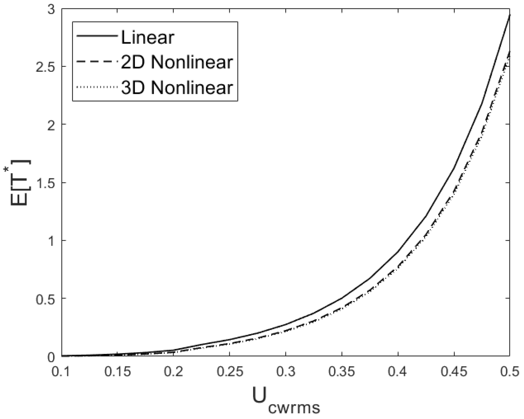
 Figure 1 for E[T*] versus Ucwrms are obtained by combining Equations (26)–(29) to cover the range of Ucwrms up to 0.5, S1 < 0.15, UR < 1 (see Appendix A), and ensuring live-bed conditions for θrms > 0.05. The results are exemplified taking n = 10, although the most appropriate statistical value of the time scale corresponding to the equilibrium scour depth is not conclusive; it is judged by the designer depending on the problem considered.
From Figure 1, it appears for random waves and current that the effect of the current is to increase the time scale, i.e., the scour develops slower when a current is added for a given wave condition. This is an inherent feature of the Larsen et al. [4] model (which the present method is based on) and is expected on physical grounds (see their paper for more details). Moreover, the time scale is smaller for 2D and 3D nonlinear waves than for linear waves; the time scale for 3D waves is slightly smaller than for 2D waves. The lower time scale for 2D nonlinear waves than for linear waves is caused by the higher wave crests for nonlinear waves, i.e., the scour develops faster for nonlinear waves than for linear waves. The smaller time scale for 3D waves than for 2D waves is due to the higher wave crests for 3D waves than for 2D waves, which is caused by the smaller wave set-down effects for short-crested than for long-crested waves as described in the last paragraph of Appendix A. Thus, the scour develops faster for 3D waves than for 2D waves.
The results can alternatively be examined by comparing the nonlinear results with the corresponding linear results for 2D and 3D waves. The nonlinear-to-linear ratios of the mean time scale is denoted as R1. Figure 2 shows R1 versus Ucwrms for 2D and 3D waves. It appears that R1 increases as Ucwrms increases, i.e., the difference between the time scales for nonlinear and linear waves decreases as the current increases; the time scale for 3D waves is slightly smaller than for 2D waves and the difference decreases as Ucwrms increases. The ratios increase from about 0.4 to about 0.9 as Ucwrms increases from 0.1 to 0.5.
Another interesting feature is to compare the 3D and 2D results. The ratio between the mean time scales for 3D and 2D nonlinear waves is denoted as R2. Figure 3 depicts R2 versus Ucwrms, showing that R2 increases as Ucwrms increases; from about 0.88 to about 0.98 as Ucwrms increases from 0.1 to 0.5. This reflects that the effect of increasing the current is to reduce the difference in time scales between 3D and 2D nonlinear waves as demonstrated in Figure 2.

4.2. Example Calculation

This example is provided to demonstrate the application of the method. The following flow conditions are considered:
  • Significant wave height, Hs = 3 m
  • Spectral peak period, Tp = 7.9 s, corresponding to ωp = 0.795 rad/s
  • Water depth, h = 10 m
  • Current speed, Uc = 0.2 m/s.
Median grain size diameter (coarse sand according to Soulsby [11]),
d50 = 1 mm,
γ = 2.65 (as for quartz sand),
Pipeline diameter, D = 1 m.
Table 1 provides the calculated quantities, where S1 and UR are given by replacing T1 and k1 with Tp and kp, respectively, due to the narrow-banded wave process. The results are for n = 10, although the statistical value of the time scale corresponding to the equilibrium scour depth is not conclusive; it is judged by the designer depending on the problem considered.
The rms value of the wave amplitude corresponds to that for a Rayleigh distribution, i.e., arms = Hs/(2 2 ). Moreover, Arms/z0 (with z0 = d50/12) exceeds 11,000, and accordingly (c,d) = (0.112,0.25). Further, θrms exceeds the threshold Shields parameter θcr ≈ 0.05 corresponding to live-bed conditions.
The expected value of the time scale due to the (1/10)th highest wave crests is considered. For linear waves and current as well as nonlinear waves and current, it is demonstrated that by adding the current, the time scale increases as discussed in Section 4.1. For waves alone the nonlinear to linear ratios for 2D and 3D waves are 0.660 and 0.620, respectively. For waves and current, the nonlinear to linear ratios for 2D and 3D waves are 0.659 and 0.615, respectively. Thus, 3D waves give slightly smaller values than 2D waves, i.e., as a result of the higher wave crests for 3D waves than for 2D waves as referred to in Section 4.1.
One should note that, for both linear and nonlinear waves, the Shields parameter θm exceeds the θcr corresponding to live-bed conditions; 3D waves give a slightly larger value than 2D waves.

5. Summary and Conclusions

A practical stochastic method is derived for the time scale of equilibrium pipeline scour due to 2D (long-crested) and 3D (short-crested) nonlinear irregular waves and current for wave-dominant flow valid for Ucwrms = Uc/(Uc + Urms) in the range 0 to 0.5, wave steepness S1 in the range 0 to 0.15, the Ursell number UR in the range 0 to 1, and live-bed conditions, i.e., θrms > 0.05.
The main conclusions are:
  • For both 2D and 3D nonlinear waves, the time scale of equilibrium scour is smaller than for linear waves for a given wave and current condition. This is caused by the higher wave crests for nonlinear waves than for linear waves, i.e., the scour develops faster for nonlinear than for linear waves.
  • The time scale for 3D nonlinear waves is smaller than that for 2D nonlinear waves. This is due to the higher wave crests for 3D waves than for 2D waves, which is caused by the smaller wave set-down effects for 3D than for 2D waves.
  • The effect of the current is to increase the time scale. The present parameter study for Hs = 3 m, Tp = 7.9 s, d50 = 1 mm shows that: (i) for 2D and 3D waves, the nonlinear-to-linear ratios of the mean time scale increase from about 0.4 to about 0.9 as Ucwrms increases from 0.1 to 0.5; (ii) the 3D nonlinear to 2D nonlinear ratio of the mean time scale increases from about 0.88 to about 0.98 as Ucwrms increases from 0.1 to 0.5.
Although the method is simple, it should be useful as a first-order approximation representing the stochastic features of the time scale for pipeline scour beneath 2D and 3D nonlinear irregular waves and current for wave-dominant flow. However, comparison with data is needed before conclusions regarding its validity can be made, but in the meantime the method should be suitable to use for the practical engineering assessment of pipeline scour for the given flow conditions.

Author Contributions

Conceptualization, D.M. and M.C.O.; methodology, D.M. and M.C.O.; software, M.C.O.; validation, D.M. and M.C.O.; formal analysis, D.M. and M.C.O.; investigation, D.M. and M.C.O.; data curation, M.C.O; writing—original draft preparation, D.M.; writing—review and editing, D.M. and M.C.O.; visualization, M.C.O. All authors have read and agreed to the published version of the manuscript.

Funding

This research received no external funding.

Institutional Review Board Statement

Not applicable.

Informed Consent Statement

Not applicable.

Data Availability Statement

Data sharing not applicable.

Acknowledgments

There is no acknowledgment.

Conflicts of Interest

The authors declare no conflict of interest.

Appendix A. Crest Height Distribution

The Forristall [10] parametric crest height distribution is based on simulations using second-order theory. The simulations were based on the Sharma and Dean [16] theory including both sum-frequency and difference-frequency effects performed both for long-crested (2D) and short-crested (3D) random waves. The results were represented by a two-parameter Weibull distribution with the cdf
P ( w c ) = 1 e x p [ ( w c 8 α ) β ] ; w c 0
that was fitted to the simulated wave data. The Weibull parameters α and β were estimated from the fit to the simulated wave data based on the wave steepness S1 and the Ursell number UR defined by, respectively,
S 1 = 2 π g H s T 1 2
U R = H s k 1 2 h 3
One should notice that Forristall provided results for S1 in the range 0 to 0.15 and UR in the range 0 to 1. Here, Hs is the significant wave height, T1 is the spectral mean period, and k1 is the wave number corresponding to T1. One should note that Hs = 2 2   arms when the wave amplitude a is Rayleigh distributed. The wave steepness and the Ursell number represent the nonlinearity of irregular waves in finite water depth. For zero steepness and zero Ursell number, the fits match the Rayleigh distribution, i.e., α = 1/ 8   = 0.3536 and β = 2, for both 2D and 3D linear waves. For 2D waves
α 2 D = 0.3536 + 0.2892 S 1 + 0.1060 U R β 2 D = 2 2.1597 S 1 + 0.0968 U R 2
and for 3D waves
α 3 D = 0.3536 + 0.2568 S 1 + 0.0800 U R β 3 D = 2 1.7912 S 1 0.5302 U R + 0.284 U R 2
The wave set-down effects are smaller for 3D waves than for 2D waves in finite water depth due to the fact that the second-order negative difference-frequency terms are smaller for short-crested than for long-crested waves (Forristall [10]). Thus, the wave crest heights are higher for 3D waves than for 2D waves.

References

  1. Myrhaug, D.; Ong, M.C.; Dyrseth, S. Time scales for scour below pipelines and around vertical piles due to nonlinear random waves. In Scour and Erosion Proceedings of the 8th International Conference on Scour and Erosion, Oxford, UK, 12–15 September 2016; CRC Press: Boca Raton, FL, USA, 2016; pp. 247–254. [Google Scholar]
  2. Whitehouse, R.J.S. Scour at Marine Structures. A Manual for Practical Applications; Thomas Telford: London, UK, 1998. [Google Scholar]
  3. Sumer, B.M.; Fredsøe, J. The Mechanics of Scour in the Marine Environment; World Scientific: Singapore, 2002. [Google Scholar]
  4. Larsen, B.E.; Fuhrman, D.R.; Sumer, B.M. Simulation of wave-plus-current scour beneath submarine pipelines. J. Waterw. Port Coast. Ocean Eng. 2016, 142, 04016003. [Google Scholar] [CrossRef] [Green Version]
  5. Zhang, Q.; Draper, S.; Cheng, L.; An, H. Time scale of local scour around pipelines in current, waves, and combined waves and current. J. Hydraul. Eng. 2017, 143, 04016093. [Google Scholar] [CrossRef]
  6. Zang, Z.; Tang, G.; Cheng, L. Time scale of scour below submarine pipeline under combined waves and currents with oblique incident angle. In Proceedings of the ASME 36th International Conference on Ocean, Offshore and Arctic Engineering, Trondheim, Norway, 25–30 June 2017. Paper No. OMAE2017-62365. [Google Scholar]
  7. Sumer, B.M.; Fredsøe, J. Scour around pipelines in combined waves and current. In Proceedings of the ASME 15th International Conference on Ocean, Offshore and Arctic Engineering, Florence, Italy, 15 June 1996; Volume 5, pp. 595–602. [Google Scholar]
  8. Myrhaug, D.; Ong, M.C. Random wave-induced scour around marine structures using a stochastic method. Mar. Technol. Eng. 2011, 1, 537–562. [Google Scholar]
  9. Myrhaug, D.; Ong, M.C. Long- and short-crested random wave-induced scour below pipelines. Proc. Inst. Civ. Eng. Marit. Eng. 2011, 164, 173–184. [Google Scholar] [CrossRef]
  10. Forristall, G.Z. Wave crest distributions: Observations and second-order theory. J. Phys. Oceanogr. 2000, 30, 1931–1943. [Google Scholar] [CrossRef]
  11. Soulsby, R.L. Dynamics of Marine Sands. A Manual for Practical Applications; Thomas Telford: London, UK, 1997. [Google Scholar]
  12. Myrhaug, D.; Holmedal, L.E.; Simons, R.R.; MacIver, R.D. Bottom friction in random waves plus current flow. Coast. Eng. 2001, 43, 75–92. [Google Scholar] [CrossRef]
  13. Catano-Lopera, Y.A.; Garcia, M.H. Geometry of scour hole, and the influence of the angle of attack on the burial of final length cylinders under combined flows. Ocean Eng. 2007, 34, 856–869. [Google Scholar] [CrossRef]
  14. Dean, R.G.; Dalrymple, R.A. Water Wave Mechanics for Engineers and Scientists; Prentice-Hall, Inc.: Upper Saddle River, NJ, USA, 1984. [Google Scholar]
  15. Ong, M.C.; Myrhaug, D.; Hesten, P. Scour around vertical piles due to long-crested and short-crested nonlinear random waves plus a current. Coast. Eng. 2013, 73, 106–114. [Google Scholar] [CrossRef]
  16. Sharma, J.N.; Dean, R.G. Second-order directional seas and associated wave forces. Soc. Pet. Eng. J. 1981, 21, 129–140. [Google Scholar] [CrossRef]
Figure 1. Expected value of nondimensional time scale for scour below pipelines for linear, 2D and 3D nonlinear random waves plus current versus Ucwrms.
Jmse 09 00114 g001
Figure 2. Nonlinear to linear ratio for 2D, R12D, waves and 3D, R13D, waves versus Ucwrms.
Jmse 09 00114 g002
Figure 3. Three-dimensional nonlinear to two-dimensional nonlinear ratio, R2, versus Ucwrms.
Jmse 09 00114 g003
Table 1. Example calculation with h = 10 m, d50 = 1 mm, D = 1 m, n = 10.
a r m s   ( m ) 1.06
k p   ( rad / m ) 0.09
S 1 0.031
U R 0.370
α 2 D , β 2 D 0.4018, 1.9468
α 3 D , β 3 D 0.3911, 1.7876
A r m s ( m ) 1.03
U r m s ( m / s ) 0.821
U c w r m s = U c / ( U c + U r m s ) 0.196
A r m s / z 0 12360
c, d0.112, 0.25
θ r m s 0.22
Time scale (waves alone)
T l i n (s)382
T 2 D (s)252
T 3 D (s)237
Time scale (waves plus current)
T l i n (s)387
T 2 D (s)255
T 3 D (s)238
Shields   parameter ,   θ m = θ c θ r m s
θ c l i n 2.83
θ m l i n 0.627
θ c n o n l i n , 2 D 3.65
θ c n o n l i n , 3 D 3.84
θ m n o n l i n , 2 D 0.807
θ m n o n l i n , 3 D 0.850
Publisher’s Note: MDPI stays neutral with regard to jurisdictional claims in published maps and institutional affiliations.

