The Role of Environmental Factors on the Fishery Catch of the Squid Uroteuthis chinensis in the Pearl River Estuary, China

Abstract

The Pearl River Estuary (PRE) is one of the major fishing grounds for the squid Uroteuthis chinensis. Taking that into consideration, this study analyzes the environmental effects on the spatiotemporal variability of U. chinensis in the PRE, on the basis of the Generalized Additive Model (GAM) and Clustering Fishing Tactics (CFT), using satellite and in situ observations. Results show that 63.1% of the total variation in U. chinensis Catch Per Unit Effort (CPUE) in the PRE could be explained by looking into outside factors. The most important one was the interaction of sea surface temperature (SST) and month, with a contribution of 26.7%, followed by the interaction effect of depth and month, fishermen’s fishing tactics, sea surface salinity (SSS), chlorophyll a concentration (Chl a), and year, with contributions of 12.8%, 8.5%, 7.7%, 4.0%, and 3.1%, respectively. In summary, U. chinensis in the PRE was mainly distributed over areas with an SST of 22–29 °C, SSS of 32.5–34‰, Chl a of 0–0.3 mg × m⁻³, and water depth of 40–140 m. The distribution of U. chinensis in the PRE was affected by the western Guangdong coastal current, distribution of marine primary productivity, and variation of habitat conditions. Lower stock of U. chinensis in the PRE was connected with La Niña in 2008.

1. Introduction

Uroteuthis chinensis (Gray, 1849) (Cephalopoda: Loginidae), a species of squid, lives in warm continental shelf waters and is widely distributed in the South China Sea (SCS), East China Sea, and Japan [1]. It is a fast-growing and highly reproductive species with a short life span (less than 7 months) and high yield (accounting for about 3/5 of the total production of the family Loliginidae) [2,3]. Because of these characteristics, the U. chinensis is considered to be an ecological opportunist that can increase the population rapidly under a suitable environment [4]. For this reason, environmental factors play a critical role in the life cycle of U. chinensis. Studies showed that cephalopods are sensitive to water temperature [5,6,7,8,9], marine primary productivity [10], and food supply [11], with temperature being the key factor affecting the population biomass and the species’ distribution [12,13]. Such conditions could impact the population dynamics by acting on the spawning activity and recruitment [7,8,14]. In the east of the Ionian Sea, the population structure and distribution of Illex coindetii depend on temperature, salinity, and circulation [15]. Any change in water temperature, chlorophyll a concentration, and salinity would affect the catch of Ommastrephes bartramii in the northwestern Pacific to a great extent [16,17]. The available studies on the U. chinensis in the SCS are all focused on biological characteristics [18,19,20], migration characteristics [21], feeding behavior [22], and resource status [23]. Studies showed that U. chinensis did not migrate on a large scale, but moved in short distances according to local water temperature. It moved northward from the SCS to the Taiwan bank and other places, with the increase of water temperature every spring, and moved southward to the SCS, looking for suitable conditions during winter [21,24]. These studies helped to understand more about the migration characters of the species, but its spatiotemporal distribution and quantitative relationship with marine environment in the Pearl River Estuary (PRE) remains unclear. It is still necessary to understand the impact of environmental variability on U. chinensis abundance in the PRE.

Due to the monsoon, the PRE has two major currents: the Guangdong Coastal Current (GCC) and the South China Sea Warm Current (SCSWC), and two coastal upwellings (in the eastern Hainan Island and the western Guangdong waters) [25,26,27]. In addition, a large amount of fresh water is discharged from the PRE every year, mixing with seawater to form the Pearl River plume [28], which radiates to the coastal waters [29]. Because of these dynamic characteristics, the PRE boasts a high primary productivity [22,30], making it one of the major fishing grounds for U. chinensis in the world [31]. Therefore, the status of U. chinensis stock in the PRE is of great research value. This study is based on six years of survey and satellite remote sensing data and looks into the relationship between the spatiotemporal distribution of the U. chinensis and some environmental factors by conducting a quantitative analysis. The possible mechanism driving the spatiotemporal distribution of U. chinensis in the PRE is also discussed. Results of this research are helpful to understand the migration characteristics, to predict the center of the fishing ground, and to protect the key habitat of the species.

2. Materials and Methods

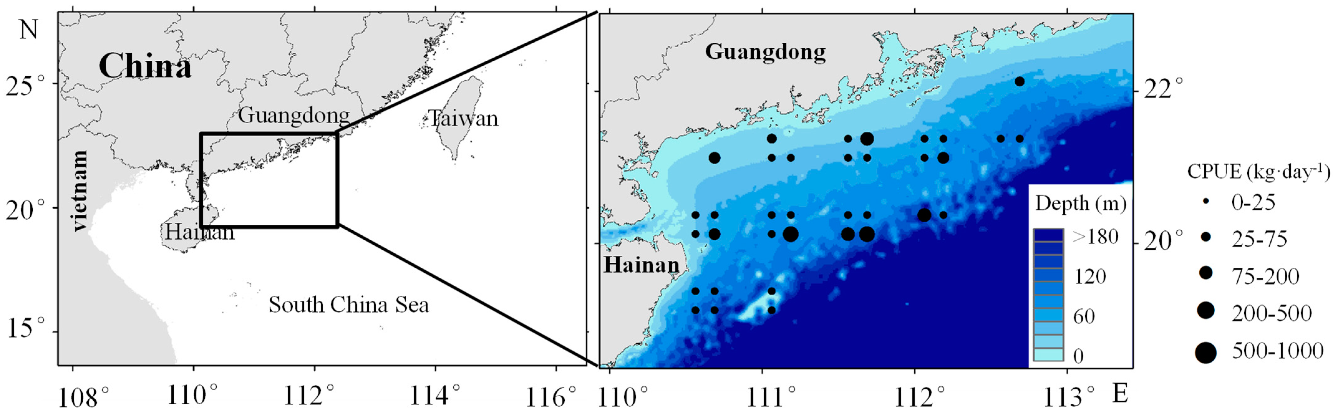
2.1. Fishery Data

The research area considered in this research is located between 19.15–22.15° N and 111.12–115.37° E (as shown in Figure 1). The U. chinensis data in the PRE was obtained from the monitoring records of light falling-net fishing vessels from August 2005 to May 2010, and the fishery data was collected at a spatial resolution of 0.25° × 0.25° and summarized in days. The dataset is composed by 359 catch data in total and 20 zero catch observations. The statistics covered longitude and latitude, operating date, voyage, catch species and catches (

Table 1. Fishing date, voyage, number of nets, number of stations and number of catch species.

Year	Month	Voyage	Number of Nets	Number of Stations	Number of Catch Species
2005	8	A1, A2, A3, A4, A5	25	10	6
	9	A5, A6, A7, A8	14	6	3
2006	8	B1, B2, B3, B4, B5	25	13	6
	9	B5, B6	8	4	4
2007	1	B14, B15	11	4	4
	2	B16	14	7	6
	3	B18	3	3	3
	8	C1, C2, C3, C4	23	10	6
	9	C4, C5, C6	21	8	6
	12	C11	9	4	4
2008	1	C12	11	3	5
	2	C14	1	1	3
	3	C14	1	1	2
	8	D1, D2, D4, D5	18	7	6
	9	D5	7	3	6
	11	D13	1	1	1
	12	D13, D14, D15	17	9	6
2009	1	D16, D17, D18	14	7	7
	2	D18, D19, D20	20	4	8
	3	D20, D21, D23	9	8	5
	5	D23	4	4	4
	8	E1, E2	21	6	6
	9	E4, E5, E6	14	8	6
	11	E11, E12	16	7	6
	12	E13, E14	16	8	6
2010	1	E15	16	6	5
	2	E17, E18, E19	14	7	4
	3	E20	6	2	5

Note: Number of catch species did not include unidentified species.

). Since 1999, China has suspended fishing activities in the SCS from 1 June to 31 July. In 2009, the closed fishing season was extended from May 16 to August 1. During these periods, ships are prohibited from fishing in the SCS [32,33] and this is why data from June to July are missing in this study.

2.2. Satellite Remote Sensing Dataremote Sensing Data

Satellite remote sensing data includes sea surface temperature (SST), sea surface salinity (SSS), sea surface chlorophyll a concentration (Chl a), current, and net primary productivity (NPP). Among them, SST was obtained from the MODIS Aqua Level 3 data products (https://oceancolor.gsfc. nasa.gov/), with temporal resolution set at 1 d and spatial resolution set at 4 km. The SSS and current data could be collected with the help of Global Ocean Physical Reanalysis Product of the Copernicus Marine Environment Management Service (CMEMS, http://marine.copernicus.eu/), with the same temporal resolution and spatial resolution of 0.083° × 0.083°. The NPP and Chl a were obtained from the CMEMS (http://marine.copernicus.eu/), with a spatial resolution of 0.25° × 0.25° and also under the same temporal conditions. The software R v.4.0.0 (R Development Core Team, 2020) was used to spatially fuse and match SST, SSS, Chl a, and fishery data, and ArcGIS 10.3 (Esri, Redlands, CA, USA) was used to plot the distribution of the flow field and NPP. Data fusion for the remote sensing data with different resolutions could be derived through the following algorithm [34]:

$${\mathrm{Ave}}_{\mathrm{j}}=\frac{{{\displaystyle \sum }}_{\mathrm{i}=1}^{\mathrm{m}}{\mathrm{value}\left(\mathrm{i}\right)}_{\mathrm{j}}}{\mathrm{m}}$$

(1)

where, ${\mathrm{Ave}}_{\mathrm{j}}$ is the average value of each environmental factor in the research area after data fusion, with a resolution of 0.25° × 0.25°; $\mathrm{m}$ is the number of pixels of each environmental factor in the area with a resolution of 0.25° × 0.25°; the value($\mathrm{i}$) is the unit pixel value in the study area, and $\mathrm{j}$ represents the fishing area, all with the same aforementioned spatial resolution of 0.25° × 0.25°.

2.3. Catch Per Unit Effort

The fish stock is expressed by catch per unit effort (CPUE), calculated with:

$$\mathrm{CPUE}=\frac{\sum \mathrm{Catch}}{\sum \mathrm{Fishing}\_\mathrm{days}}$$

(2)

where, $\sum \mathrm{Catch}$ (units: tons [t]) is the sum of catches within a fishing grid of 0.25° × 0.25°. $\sum \mathrm{Fishing}\_\mathrm{days}$ is the sum of fishing days for the fishing vessel in the fishing grid, and the unit of $\mathrm{CPUE}$ is marked as t day⁻¹. Day was chosen as the time step in grouping CPUE for each fishing grid.

2.4. Clustering Fishing Tactics

Clustering Fishing Tactics (CFT) is a method widely used to identify fishing tactics from commercial data by capturing component records through clustering techniques [35,36,37]. A data matrix containing CPUE records of each species was constructed in the research area, and then the data was normalized to the relative proportion according to weight to eliminate the impact of catch rate. Next, the square root transformation of the standardized matrix was carried out so that the species with lower dominance could make similar contributions to the catch composition. After the initial steps, a principal component analysis (PCA) was applied to the multidimensional data matrix. It is worth noting that most of the changes in the data were explained by the first few axes of the PCA-converted data. Finally, all PCA axes were reserved for clustering analysis [36,38,39]. In this study, CFT identified the fishing tactics adopted by fishermen, so as to evaluate the impact of their behavior and other human factors in fishing activities on the stock of U. chinensis. R 4.0.0 (R Development Core Team, 2020) was used to conduct PCA and cluster analysis on fishery data, and the fishing tactic (FT) result taken as one of the explanation factors of GAM [38]. The fishing strategy was converted into a numerical variable for processing in order to calculate its impact on the change of CPUE.

2.5. GAM Analysis

A Generalized Additive Model (GAM) is a nonparametric extension of the generalized linear model [40]. In fishery, GAM is widely used in quantitative analysis of the relationship between fishery resources and environmental factors, which is a non-linear regression [13,41,42]. The distribution of Tweedie was determined in 1984 [43], and it is suitable to describe nonnegative and biased random variables. The process includes several common important distributions (p = 0 normal distribution, p = 1 Poisson distribution, 1 < p < 2 Poisson gamma composite distribution, p = 2 gamma distribution, p = 3 inverse Gaussian distribution) [44]. If 1 < p < 2, it is considered that Tweedie distribution is suitable for analyzing CPUE [35,45]. This specific method is a special probability distribution part of the exponential distribution family, generally expressed by ${\mathrm{Tw}}_{\mathrm{P}}(\mathsf{\theta },\mathsf{\phi })$ and completely determined by the variance function $\mathrm{V}\left(\mathsf{\mu }\right)={\mathsf{\mu }}^{\mathit{P}}$, where θ is a gauge parameter and φ is a decentralized parameter [43,44]. Since Tweedie distribution still belongs to the exponential distribution family, the statistical relationship model between the corresponding variables and the influencing factors can be established within the framework of the generalized linear model [46]. To avoid the zero-catch problem of CPUE, the GAM was applied together with the Tweedie distribution to analyze the environmental influence on the U. chinensis stock [45]. The GAM basic model constructed in this study is:

$$\left\{\begin{array}{c}{\mathrm{CPUE}~\mathrm{TW}}_{\mathit{p}}(\mathsf{\theta },\mathsf{\phi })\\ \ln \left({\mathsf{\mu }}_{\mathrm{CPUE}}\right)=\mathrm{s}\left(\mathrm{Month},\mathrm{SST}\right)+\mathrm{s}\left(\mathrm{Month},\mathrm{Depth}\right)+\mathrm{s}\left(\mathrm{Chl} \mathrm{a}\right)+\mathrm{s}\left(\mathrm{SSS}\right)+\mathrm{s}\left(\mathrm{FT}\right)+\mathrm{s}\left(\mathrm{year}\right)+\mathsf{\epsilon }\end{array}\right.$$

(3)

where, ${\mathsf{\mu }}_{\mathrm{CPUE}}$ is the mean of Tweedie distribution of CPUE; $\mathrm{s}$ is the function of smoothing splines; $\mathrm{s}\left(\mathrm{Month},\mathrm{SST}\right)$ represents the interaction effect of month and SST; $\mathrm{s}\left(\mathrm{Month},\mathrm{Depth}\right)$ is the interaction effect of month and water depth. Furthermore, $\mathrm{s}\left(\mathrm{Chl} \mathrm{a}\right)$ stands for the effect of Chl a; $\mathrm{s}\left(\mathrm{SSS}\right)$ is the effect of SSS; $\mathrm{s}\left(\mathrm{FT}\right)$ is the effect of fishing tactic; $\mathrm{s}\left(\mathrm{year}\right)$ is the effect of year. Finally, $\mathsf{\epsilon }$ represents the model error. The GAM was constructed and tested by the ‘mgcv’ package of software R v.4.0.0 [47]. A forward stepwise method was used to select variables that have significant influence on the model, so the specific expression of GAM could be determined.

3. Results

3.1. Analysis of Fishing Tactics

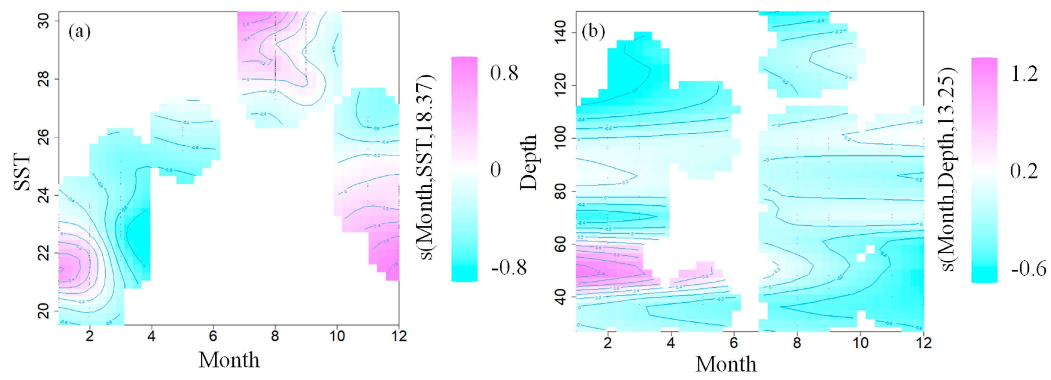
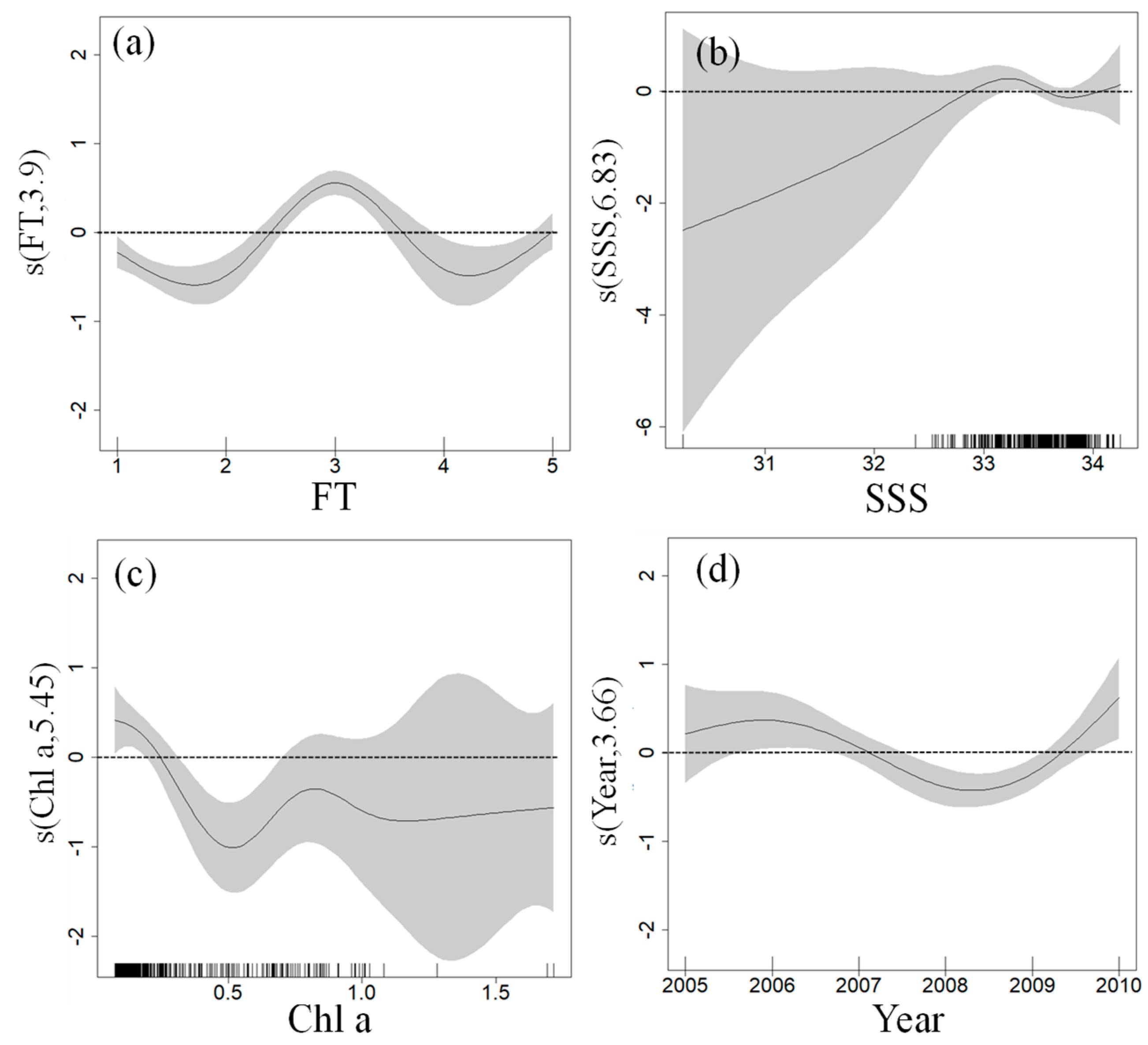
On the basis of the cluster analysis, the catch matrix was identified in five groups, assigned to five different fishing tactics. Among them, FT1 and FT3 mainly included offshore pelagic economic fishes. FT1 was represented by Decapterus (77.08%) and FT3 represented by U. chinensis (62.02%). FT2 mainly included middle and demersal fishes, represented by Trichiurus haumela (75.57%). Furthermore, FT4 mainly considers unidentified species (68.44%), and had a high catch of U. chinensis (30.98%), without a bycatch of Decapterus and Scombridae. Last, the majority of FT5 included oceanodromous fishes, represented by Scombridae (49.04%), mainly composed of Katsuwonus pelamis (

Table 2. Major catch species and proportion under five fishing tactics (FTs).

Species	FT1	FT2	FT3	FT4	FT5
U. chinensis	9.00	13.37	62.02 *	30.98	13.77
Scombridae	1.88	1.40	2.52	0.00	49.04 *
Decapterus	77.08 *	8.43	18.22	0.00	8.08
Trichiurus haumela	2.39	75.57 *	9.74	0.58	10.18
Rastrelliger kanagurta	5.86	0.00	0.63	0.00	2.17
Formio niger	0.32	0.38	0.78	0.00	11.04
Sparidae	1.69	0.00	1.32	0.00	1.08
Navodon	1.38	0.06	1.83	0.00	3.48
unidentified species	0.39	0.79	2.93	68.44 *	1.17

* indicates species with the highest weight proportion in each net.

).

3.2. GAM Analysis

The cumulative bias explanatory rate of spatiotemporal and environmental factors on U. chinensis CPUE was obtained by using the GAM to fit and predict the effect of adding variables to the model (Table 2). The explanatory variables selected for the model included the interaction effect of month and sea surface temperature (Month, SST), the interaction effect of month and water depth (Month, Depth), chlorophyll a concentration (Chl a), sea surface salinity (SSS), fishing tactic (FT), and year (Year). The cumulative bias explanatory rate of these factors for U. chinensis CPUE was 63.1%, and the correlation coefficient R² was 0.51 (

Table 3. Deviance analysis for the general additive models (GAMs) fitted to U. chinensis Catch Per Unit Effort (CPUE).

Influencing Factors (p = 1.7)	AIC	GCV	Adjusted R2	Deviance Explained (%)	Residual Deviance
CPUE~NULL	5122.37	63.02	0	0.0	22,498.85
CPUE~s(Month, SST)	4926.65	53.46	0.14	26.7	16,500.28
CPUE~s(Month, SST) + s(Chl a)	4896.35	52.05	0.17	30.7	15,581.08
CPUE~s(Month, SST) + s(Chl a) + s(SSS)	4831.30	48.19	0.23	38.4	13,864.01
CPUE~s(Month, SST) + s(Chl a) + s(SSS) + s(Month, Depth)	4715.83	41.56	0.37	51.6	10,885.54
CPUE~s(Month, SST) + s(Chl a) + s(SSS) + s(Month, Depth) + s(FT)	4616.75	34.62	0.48	60.1	8969.72
CPUE~s(Month, SST) + s(Chl a)+s(SSS)+s(Month, Depth) + s(FT) + s(Year)	4587.61	33.02	0.51	63.1	8295.15

).

In GAMs, the contribution of selected factors to CPUE represents the influencing degree of each factor on U. chinensis CPUE (

Table 4. Contribution and significance test in GAMs.

Variables	Contribution (%)	d.f.	Pr(F)	Pr(chi)
s(Month, SST)	26.7	27.9	< 0.001	< 0.001
s(Month, Depth)	12.8	18.7	< 0.001	< 0.001
s(FT)	8.5	2.5	< 0.001	< 0.001
s(SSS)	7.7	7.5	< 0.001	< 0.001
s(Chl a)	4.0	6.3	0.015	0.013
s(Year)	3.1	5.0	< 0.001	< 0.001

). Among them, the interaction effect of month and SST was the most influencing factor, with a contribution of 26.7%; followed by the interaction effects of month and depth, FT, SSS, Chl a, and year, with contribution of 12.8%, 8.5%, 7.7%, 4.0%, and 3.1%, respectively. The Chi-square and F test showed that the selected explanatory variables were significantly correlated with CPUE (p < 0.05; Table 4).

The interaction effect of month and SST based on GAM showed that from December to February in the waters with SST of 21–22 °C and from July to August in the waters with SST of 28–30 °C, month and SST had a positive effect on U. chinensis CPUE, which showed an upward trend in this range (Figure 2a). The result of the interaction effect of month and depth indicates that the positive effect of month and water depth on U. chinensis CPUE was the highest in the area of 40–60 m from January to June, when U. chinensis CPUE increased (Figure 2b). In other months (from July to December), no obvious tendency towards depth was shown. The species was evenly distributed in the water depth of 40–130 m.

The influence of such factors as FT, SSS, Chl a, and year on the U. chinensis CPUE was analyzed on the basis of GAMs (Figure 3). Results showed that in FT1–FT3, the U. chinensis CPUE increased with the increase of FT; in FT3-FT5, the U. chinensis CPUE decreased with the increase of FT. FT3 had a positive effect on U. chinensis CPUE (Figure 3a). When the SSS was in 30.0–33.0‰, the U. chinensis CPUE increased together with the, SSS but when the SSS was in 33–34‰, it got diminished with the increase of SSS. It was also observed that SSS in 33.0‰ had a positive effect on U. chinensis CPUE (Figure 3b). When Chl a was 0–0.5 mg × m⁻³, the U. chinensis CPUE decreased as the levels of Chl a enhanced. Differently, when Chl a was 0.5–0.8 × mg m⁻³, the U. chinensis CPUE increased in accordance with Chl a. Another possibility that was observed involved Chl a in the range of 0.8–2 mg × m⁻³, and the U. chinensis CPUE decreasing with it. Furthermore, Chl a of 0–0.2 mg × m⁻³ had a positive effect on U. chinensis CPUE (as shown in Figure 3c). From 2005 to 2008, the U. chinensis CPUE decreased as the years passed. Oppositely, from 2008 to 2010, the U. chinensis CPUE increased with the year. Being more specific, the year of 2008 had a negative effect on U. chinensis CPUE (Figure 3d).

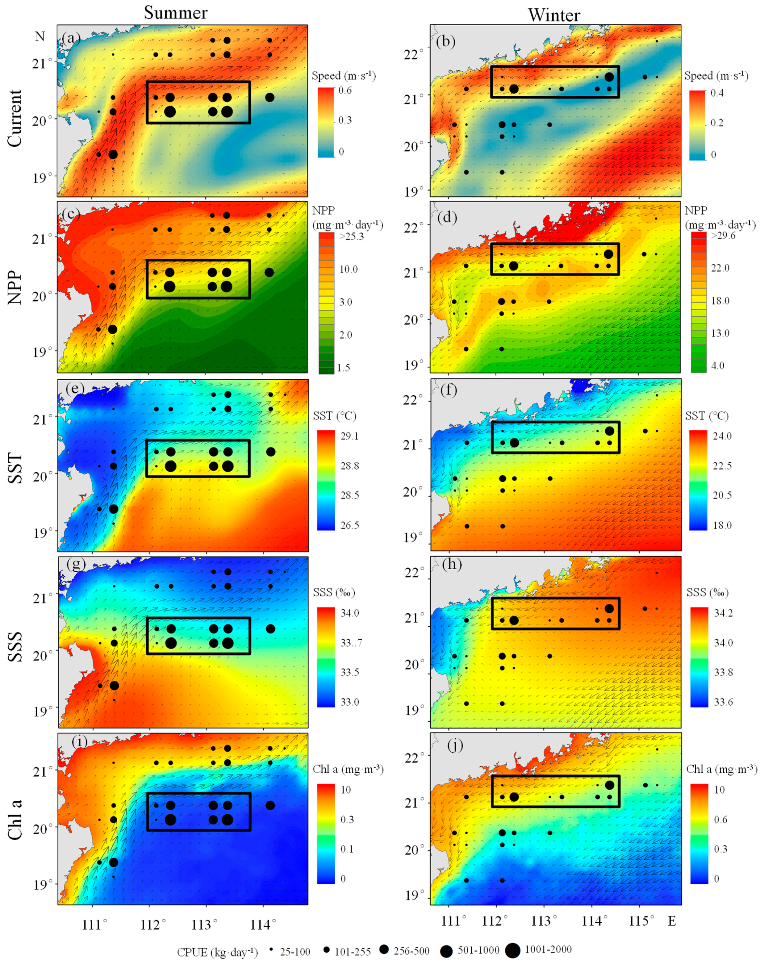
3.3. Seasonal Variation of U. chinensis

In summer (from August to September in that zone), along the outside of the SCSWC, the SST was higher and Chl a was lower. Furthermore, SSS in the area were distributed in a ladder shape along the PRE to the SCS (Figure 4e,g,i). The fishing grounds of U. chinensis in the PRE were mainly distributed in the sea area at a longitude of 111–114° E and latitude of 19.5–20.5° N. High CPUEs (1001–2000 kg × day⁻¹) were majorly spread in the sea area with a velocity of about 0.3 m × s⁻¹, NPP of 3–5 mg × m⁻³·day⁻¹, SST of 28.8–29.0 °C, SSS of 33.5–33.6‰, and Chl a of 0–0.1 mg × m⁻³ (Figure 4a,c,e,g,i).

In winter (from December to February), SSS gradually decreased from east to west along the GCC, together with Chl a that also got slowly reduced along the coast of Guangdong to the open sea. Major U. chinensis concentrated in the area outside the GCC with higher SST and lower Chl a (Figure 4f,h,j). The fishing grounds of U. chinensis in the PRE were mainly distributed in the sea area at a longitude of 111–115.5 °E and latitude of 19–22 °N. High CPUEs (501–1000 kg × day⁻¹) were allocated in the sea area with a current velocity of 0.2 m × s⁻¹, NPP of 17–19 mg × m⁻³·day⁻¹, SST of 21.0–23.0 ℃, SSS of 34.0–34.1‰, and Chl a of 0.4–0.6 mg × m⁻³ (Figure 4b,d,f,h,j).

4. Discussion

4.1. Relationship between the U. chinensis and Marine Environment

The fact that water temperature affected each stage of the life history of squid from embryos, juveniles to adults [7,14,48], was one of the important factors indicating its spatiotemporal distribution [12,41]. It was verified that temperature variation could significantly change the growth and development of the reproductive systems of squid [49,50]. Warmer temperatures may lead to the rapid development of embryos and juveniles, shorten their hatching period [48], and thus affect the recruitment of the squid population [7]. In addition, the water temperature affected fish stock in some specific months [50,51]. Therefore, the interaction effect of month and temperature was considered for GAM fitting. Results showed that the interaction effect of SST and month had the greatest impact on the U. chinensis CPUE (with a contribution of 26.7%; Table 4). SST played a positive role on the U. chinensis CPUE in summer (from August to September; Figure 3a). This happened partly because warm water speeded up the embryonic development and the growth process of juvenile squid [14]. In addition, due to the short life span of the squid, its abundance directly depended on the recruitment capacity of the current year [52]. The CPUE increased if the number of individuals hatched in spring and summer—under the appropriate water temperature from August to September. In the East China Sea, a higher SST in summer, especially at 29 °C, could improve the growth rate and reproductive capacity of U. edulis [50]. In winter (from December to February), SST showed a positive effect on the U. chinensis CPUE (Figure 2a). This might be related to the thermophilic-feeding migration of the species, hatched in the autumn, considered to be the spawning season. In the fishing grounds in the south of the Taiwan Strait, the U. chinensis migrated to warmer areas for feeding every winter [53]. According to its age analysis caught by fishing vessels [2,54], generally, U. chinensis will become the target size of the fishing vessel and be captured when they grow to be 2–5 months old. Therefore, from December to February, SST 21–23 °C can be one of the indicators for the distribution of U. chinensis in the PRE.

It was also observed that the levels of salinity affected the physiological activities of marine organisms by changing their osmotic pressure [55]. The GAM analysis showed that SSS contributes 7.7% to the U. chinensis stock (Table 4). The species was mainly distributed in the waters with a SSS of 32.5–34‰ (Figure 3b). The narrow suitable salinity range for U. chinensis is mainly a result of the poor osmolality regulation mechanism of most cephalopods, since it is a stenohaline species and tends to prefer medium or high salinity environment [31]. Moreover, the salt levels also affected the survival rate of squid embryos, consequently affecting the squid stock as well [56]. When the salinity was lower than 32‰ or higher than 38‰, the survival rate of squid embryos was greatly reduced. It is also noteworthy that large fluctuations in salinity may cause the eggs to die [57].

When it comes to the chlorophyll a concentration, it reflected the phytoplankton in stock in the sea area. As the major feeding source of zooplankton and some marine organisms, phytoplankton is an important part of marine primary productivity and reflects the primary productivity level of the sea area [42,58]. The GAM analysis indicated that the contribution of Chl a to the U. chinensis stock was 4.0% (Table 4). The trophic level of the U. chinensis was 2.7–3.6 [18], as it mainly fed on fish and cephalopods [59]. In the PRE, U. chinensis tended to live in waters with low Chl a (Figure 3c), and the U. chinensis CPUE decreased, while the Chl a did the opposite and kept increasing. This might be related to the hysteresis in the response of the species to chlorophyll a [12]. In addition, the U. chinensis vision was affected by the transparency of sea water. In the southeast waters of Brazil, the abundance of U. chinensis was negatively correlated with the chlorophyll a concentration, as the sea area with a low concentration of the pigment had a high transparency, causing U. chinensis to be easier to be attracted by baits. The consequence of all of this was an increase in the catch [8].

4.2. Relationship between U. chinensis and CFT

The GAM analysis also showed that the contribution of fishing tactics to the U. chinensis CPUE was 8.5% (Table 4). Considering that the northern SCS is a typical sea area with multi-species fishes, and with a variety of resource species and complex composition [60,61], fishermen might target species on the basis of economic benefits and the condition of the sea they are acting on. The major species caught in the PRE were U. chinensis (FT3), Euthynnus alletteratus (FT5), Decapterus (FT1), and hairtail (FT2). The examination of these five clustering fishing tactics showed that four clustering fishing tactics (FT1, FT2, FT3, FT5) were aimed at a single species (Table 2). This might be due to the spatial segregation of habitats of major commercial species in the PRE. The spatial segregation of habitat usually led to a negative correlation between the CPUE of the bycatch species and target species [62]. Studies on habitat utilization and feeding behavior of four different species of squid (U. duvaucelii, U. edulis, U. chinensis and Loliolus uyii) in the northern SCS showed that although the feeding strategy was similar, their habitats did not overlap. This spatial segregation could reduce their competition for resources and buffer their trophic interactions, thus increasing the possibility of the species coexisting in the region [22].

4.3. Spatiotemporal Variation of U. chinensis

Water depth also affected the spawning activity of squid by changing the level of dissolved oxygen in water [63]. Here, it is important to consider that there is an appropriate season when squid migrate to shallow waters for spawning [31,41,64]. The GAM analysis showed that the interaction effect of month and depth contributes 12.8% to the U. chinensis CPUE (Table 4) and that the species was widely distributed in the water depth of 40–140 m. From January to March, in waters that are 40–60 m deep, water depth played a positive role on the U. chinensis CPUE (Figure 2b). This phenomenon might be related to the mass spawning behavior of the U. chinensis. In the coastal waters of Guangdong Province, the period between February to May was the peak spawning period of the U. chinensis as they migrate to the shallow sea to spawn [31]. This seasonal spawning activity led to a regional fishing season [53]. U. chinensis can spawn in any season, but the peak happens when there is a suitable and appropriate environment for the process to occur [2,65]. In the PRE, the SST during January and March ranged from 20–24 °C, meeting the spawning requirements of the species [31]. This also resulted in an increase of its CPUE in waters from 40–60 m depth and within the period from January to March (Figure 2a,b). From August to November, the water in the PRE became warmer, boosting the metabolism of the U. chinensis, and driving their demand for food, which led to increased feeding activity. Moreover, warmer temperatures provided a more suitable condition for the early lives of U. chinensis [14,48], partly leading to a more even distribution of the animals along the study area (Figure 2b).

The GAM analysis also provided that the contribution of interannual variation to the fluctuation of U. chinensis CPUE was 3.1%. The CPUE decreased significantly from 2007 to 2008 (Figure 3d). It was also observed that large-scale climate variability, such as the North Atlantic Oscillation, affects the abundance of a myriad squid species (e.g., Illex illecebrosus, Loligo pealeii) [66]. For instance, the yield of Loligo Opalesens decreased after the El Nino-Southern Oscillation event occurred in the Southern California Bay [67]. La Niña also affected the recruitment of squid by changing the environment of spawning grounds, see also [16]. In Antarctica, squid got more abundant in the sea area, due to a change in the water temperature caused by La Niña [68]. In the offshore area of the sea area, this resulted in less squid abundance [69]. From August 2007 to April 2008, a La Niña event [70] was formed, which led to the decrease of SST in the SCS. Furthermore, the center of the Symlectoteuthis oualaniensis fishing ground in the Xisha-Zhongsha waters shifted to the south by about 2° N [13]. Furthermore, La Niña also made rain happen more often and also affected the wind speed in the region [70], as well as the wind speed that strengthened the wave field in the area in terms of cycle and frequency. This new characteristic of the wave field disturbed the near shore spawning grounds, deviating mature fish swarm from these areas, imposing a negative impact on the fish stock [71]. Therefore, it can be said that the decrease of U. chinensis stock in 2008 may be connected with La Niña.

4.4. Analysis of Seasonal Variation of U. chinensis

Current and wind fields are also considered important factors in the life span of cephalopods [72] that affect the variation of water temperature and salinity [73,74], and may further change the composition, structure, and thermophilic characteristics of fish communities [75]. The fronts and vortices formed by the flow field served as key spawning habitats for pelagic fishes [76]. Fishing grounds with abundant resources can be formed around the large-scale current, such as the Illex argentinus in the southwest Atlantic Ocean, the Ommastrephes bartramii in the North Pacific Ocean, and the Todarodes pacificus in the waters around Japan, all of them distributed in the western boundary current [1,77]. The current velocity was an important factor for the success of fish migration and feeding [78]. Studies showed that in summer, driven by the southwest monsoon [79], SCSWC was stronger in the PRE. In the southern boundary of the current where the velocity was about 0.3 m × s⁻¹, a number of areas with high U. chinensis CPUE were formed (Figure 4a). In winter, under the control of the northeast monsoon [27], the southwesterly Guangdong Coast Current (GCC) started to form. At the southern boundary of the current where the velocity is 0.2 m × s⁻¹, several areas with high U. chinensis CPUE were identified. In the PRE, the current velocity in different seasons can be considered one of the indicators to predict the distribution of U. chinensis fishing grounds.

As one of most important indicators of the nutritional potential of the basic links in the marine food chain, primary productivity plays an important role in marine ecology [80]. Its size determines the potential yield of marine fishery [81] and can be used to indicate the spatiotemporal variation of fish stock [10]. In the spawning season, high NPP suggests high plankton biomass, an important feature for the growth and recruitment of juvenile fish. In the catching season, the NPP acts like the comprehensive index of biological concentration of squid bait, and the interaction between them can directly affect the annual stock level of squid [82]. A significant correlation between the interannual stock variation of Ommastraphes bartrami and the average NPP was observed in spawning and catching months [82]. Hence, high primary productivity areas caused by strong upwelling were generally considered as potential spawning grounds [83]. However, the relationship between primary productivity and squid was also affected by the cascade effect. The increase of primary productivity did not act on squid directly, and high levels of primary productivity can eventually lead to the increase of both prey and predator. On the western coast of California, the increase of primary productivity anomaly led to the decline of squid stock after three months [84]. In the PRE, the suitable NPP of U. chinensis differed depending on the month. In summer, the high resource was mainly distributed in the narrow zone with a NPP of about 3–5 mg × m⁻³day⁻¹, while in winter it was mainly distributed in the water area with a NPP of 16–19 mg m⁻³day⁻¹ (Figure 4c,d).

In summer, the PRE was majorly affected by the SCSWC and the Pearl River plume (PPP) (Figure 4) and the environmental characteristics on both sides of the SCSWC were significantly different. During this period, the PRE was in the wet season and a great amount of fresh water from land discharged to the PRE [85]. Therefore, the distribution of SSS was mainly affected by the PPP. The U. chinensis was mainly distributed in the waters outside the SCSWC, located in the area where the diluted water from PRE and the high salinity water from SCS were mixed. In winter, the area was mainly influenced by GCC [85]. In this case, the species could be found in the area where high salinity and low salinity seawater mixed and its CPUE was lower than in summer (Figure 4). Therefore, the relationship between the U. chinensis and the environment was similar in winter and summer, and it was adjusted by the changes of currents and marine environments. In the SCS, the high Sthenoteuthis oualaniensis CPUE was concentrated in the area with a high SST. With the seasonal warming, the same species shifted to lower latitudes [13], similar to the migration characteristics of the U. chinensis presented throughout this study. In addition, the U. chinensis CPUE in summer was higher than in winter, an observation that is consistent with the peak fishing season of squid in the Beibu Gulf [86]. However, in the Gulf of Cadiz, according to the bottom trawl survey, the abundance of Loligo vulgaris was the highest in autumn [52]. This difference may be related to the different fishing methods, latitude, and spawning periods, which need to be further explored in related future research.

5. Conclusions

This paper studied the effect of marine environmental factors on the spatiotemporal distribution of U. chinensis in the PRE on the basis of the long-term satellite remote sensing and survey data. It was observed that the interaction effect of SST and month was the most important environmental factor affecting the U. chinensis stock (accounting for 26.7% of the U. chinensis CPUE), followed by the interaction effect of depth and month (accounting for 12.8% of the U. chinensis CPUE). In the PRE, U. chinensis was mainly distributed in the sea area with an SST of 22–29 °C, SSS of 32.5–34‰, Chl a of 0–0.3 mg × m⁻³, and water depth of 40–140 m. It is important to clarify that, in this study, only data related to SST, SSS, Chl a, depth, NPP, and current available from satellite remote sensing were analyzed. Morphological characteristics such as body length, age, and parameters such as dissolved oxygen and transparency were not considered and represent possibilities for follow-up studies to improve the accuracy of the model, thus providing a scientific basis for protecting the habitat of the U. chinensis.

References

1. Roper, C.F.E.; Sweeney, M.J.; Nauen, C.E. FAO Species Catalogue. Cephalopods of the World; FAO Fisheries Synopsis: Rome, Italy, 1984; Volume 3, pp. 1–247. [Google Scholar]
2. Sukramongkol, N.; Tsuchiya, K.; Segawa, S. Age and maturation of Loligo duvauceli and l. Chinensis from Andaman sea of Thailand. Rev. Fish. Biol. Fish. 2006, 17, 237–246. [Google Scholar] [CrossRef]
3. Editorial Committee of Fauna Sinica, Academia Sinica. Fauna Sinica: Phylum Mollusca Class Cephalopode; Science Press: Beijing, China, 1988; pp. 92–94. [Google Scholar]
4. Arkhipkin, A.I.; Rodhouse, P.G.K.; Pierce, G.J.; Sauer, W.; Sakai, M.; Allcock, L.; Arguelles, J.; Bower, J.R.; Castillo, G.; Ceriola, L.; et al. World squid fisheries. Rev. Fish. Sci. Aquac. 2015, 23, 92–252. [Google Scholar] [CrossRef] [Green Version]
5. Robin, J.P.; Denis, V. Squid stock fluctuations and water temperature: Temporal analysis of English channel Loliginidae. J. Appl. Ecol. 1999, 36, 101–110. [Google Scholar] [CrossRef]
6. Roberts, M.J.; Downey, N.J.; Sauer, W.H. The relative importance of shallow and deep shelf spawning habitats for the South African chokka squid (Loligo reynaudii). ICES J. Mar. Sci. 2012, 69, 563–571. [Google Scholar] [CrossRef] [Green Version]
7. Challier, L.; Royer, J.; Pierce, G.J.; Bailey, N.; Roel, B.; Robin, J.-P. Environmental and stock effects on recruitment variability in the english channel squidloligo forbesi. Aquat. Living. Resour. 2005, 18, 353–360. [Google Scholar] [CrossRef]
8. Postuma, F.A.; Gasalla, M.A. On the relationship between squid and the environment: Artisanal jigging for loligo plei at São Sebastião island (24°s), southeastern brazil. ICES J. Mar. Sci. 2010, 1353–1362. [Google Scholar] [CrossRef] [Green Version]
9. Li, J.J.; Wang, J.T.; Chen, X.J.; Lei, L.; Guan, C.T. Spatio-temporal variation of Ommastrephes bartramii resources (winter & spring groups) in Northwest Pacific under different climate modes. South China Fish. Sci. 2020, 16, 62–69. [Google Scholar]
10. Ichii, T.; Mahapatra, K.; Sakai, M.; Wakabayashi, T.; Okamura, H.; Igarashi, H.; Inagake, D.; Okada, Y.J.M.E.P. Changes in abundance of the neon flying squid Ommastrephes bartramii in relation to climate change in the central North Pacific Ocean. Mar. Ecol. Prog. Ser. 2011, 441, 151–164. [Google Scholar] [CrossRef] [Green Version]
11. Smith, J.M.; Pierce, G.J.; Zuur, A.F.; Martins, H.; Clara Martins, M.; Porteiro, F.; Rocha, F. Patterns of investment in reproductive and somatic tissues in the loliginid squid Loligo forbesii and Loligo vulgaris in Iberian and Azorean waters. Hydrobiologia 2011, 670, 201–221. [Google Scholar] [CrossRef]
12. Yu, J.; Hu, Q.; Tang, D.; Zhao, H.; Chen, P. Response of Sthenoteuthis oualaniensis to marine environmental changes in the north-central south China Sea based on satellite and in situ observations. PLoS ONE 2019, 14, e0211474. [Google Scholar] [CrossRef] [Green Version]
13. Yu, J.; Hu, Q.; Tang, D.; Chen, P. Environmental effects on the spatiotemporal variability of purpleback flying squid in Xishazhongsha waters, South China sea. Mar. Ecol. Prog. Ser. 2019, 623, 25–37. [Google Scholar] [CrossRef]
14. David, J.A.; Simeon, H.; John, R.B. Predicting the recruitment strength of an annual squid stock: Loligo gahi around the falkland islands. Can. J. Fish. Aquat. Sci. 2000, 57, 2479–2487. [Google Scholar] [CrossRef]
15. Lefkaditou, E.; Politou, C.-Y.; Palialexis, A.; Dokos, J.; Cosmopoulos, P.; Valavanis, V.D. Influences of environmental variability on the population structure and distribution patterns of the short-fin squid Illex coindetii (cephalopoda: Ommastrephidae) in the eastern Ionian sea. Hydrobiologia 2008, 612, 71–90. [Google Scholar] [CrossRef]
16. Chen, X.J.; Zhao, X.H.; Chen, Y. Influence of el niño/la niña on the western winter–spring cohort of neon flying squid (Ommastrephes bartramii) in the northwestern Pacific Ocean. ICES J. Mar. Sci. 2007, 64, 1152–1160. [Google Scholar] [CrossRef] [Green Version]
17. Yu, W.; Chen, X.; Yi, Q.; Chen, Y.; Zhang, Y. Variability of suitable habitat of western winter-spring cohort for neon flying squid in the northwest pacific under anomalous environments. PLoS ONE 2015, 10, e0122997. [Google Scholar] [CrossRef] [Green Version]
18. Yan, Y.R.; Li, Y.Y.; Yang, S.Y.; Wu, G.R.; Tao, Y.J.; Feng, Q.B.; Lu, H.S. Biological characteristics and spatial—Temporal distribution of mitre squid, Uroteuthis chinensis, in the Beibu gulf, South China Sea. J. Shellfish. Res. 2013, 32, 835–844. [Google Scholar] [CrossRef]
19. Jin, Y.; Li, N.; Chen, X.; Liu, B.; Li, J. Comparative age and growth of Uroteuthis chinensis and Uroteuthis edulis from china seas based on statolith. Aquac. Fish. 2019, 4, 166–172. [Google Scholar] [CrossRef]
20. Jin, Y.; Lin, F.; Chen, X.; Liu, B.; Li, J. Microstructure comparison of hard tissues (statoliths, beaks, and eye lenses) of Uroteuthis chinensis in the South China Sea. B. Mar. Sci. 2019, 95, 13–26. [Google Scholar] [CrossRef]
21. Chen, F.J. Survey of mitre squid resource in Minnan-Taiwan bank fishing ground and suggestions for sustainable utilization. Fish. Inf. Strategy 2016, 31, 270–277. [Google Scholar] [CrossRef]
22. Lin, D.; Zhu, K.; Qian, W.; Punt, A.E.; Chen, X. Fatty acid comparison of four sympatric loliginid squids in the northern south china sea: Indication for their similar feeding strategy. PLoS ONE 2020, 15, e0234250. [Google Scholar] [CrossRef]
23. Li, Y.; Sun, D.Y. Biological characteristics and stock changes of loligo chinensis gray in Beibu Gulf, South China Sea. Hubei Agric. Sci. 2011, 50, 2716–2719. [Google Scholar] [CrossRef]
24. Gong, J.K. A study on the migratory distribution and biological characteristics of the Uroteuthis chinensis in Minnan-Taiwan Shoal fishing ground. J. Fujian Fish. 1981, 15–26. [Google Scholar] [CrossRef]
25. Ji, X.; Sheng, J.; Zheng, J.; Zhang, W. Numerical study of seasonal circulation and variability over the inner shelf of the northern South China Sea. Ocean. Dynam. 2015, 65, 1103–1120. [Google Scholar] [CrossRef]
26. Xu, J.D.; Cai, S.Z.; Xuan, L.L.; Qiu, Y.; Zhu, D.Y. Study on coastal upwelling in eastern Hainan Island and western Guangdong in summer, 2006. Acta. Oceanol. Sin. 2013, 35, 11–18. [Google Scholar]
27. Shu, Y.; Wang, Q.; Zu, T. Progress on shelf and slope circulation in the northern South China Sea. Sci. China. Earth. Sci. 2018, 61, 560–571. [Google Scholar] [CrossRef]
28. Ye, H.; Chen, C.; Sun, Z.; Tang, S.; Song, X.; Yang, C.; Tian, L.; Liu, F. Estimation of the primary productivity in pearl river estuary using modis data. Estuar. Coast. 2014, 38, 506–518. [Google Scholar] [CrossRef]
29. Gan, J.; Li, L.; Wang, D.; Guo, X. Interaction of a river plume with coastal upwelling in the northeastern South China Sea. Cont. Shelf. Res. 2009, 29, 728–740. [Google Scholar] [CrossRef]
30. Chen, F.; Zhou, X.; Lao, Q.; Wang, S.; Jin, G.; Chen, C.; Zhu, Q. Dual isotopic evidence for nitrate sources and active biological transformation in the northern South China Sea in summer. PLoS ONE 2019, 14, e0209287. [Google Scholar] [CrossRef]
31. Chen, X.J. Cephalopods of the World; China Ocean Press: Beijing, China, 2009; pp. 1178–1179. [Google Scholar]
32. Wu, Z. Review and reflection on the ten years of fishing ban in the South China Sea. China Fish. 2008, 8, 4–6. [Google Scholar]
33. Yu, J.; Hu, Q.W.; Yuan, H.R.; Chen, P.M. Effect assessment of summer fishing moratorium in Daya Bay based on remote sensing data. South China Fish. Sci. 2018, 14, 1–9. [Google Scholar] [CrossRef]
34. Fu, D.Y.; Tang, D.L.; Levy, G. The impacts of 2008 snowstorm in China on the ecological environments in the Northern South China Sea. Geomat. Nat. Haz. Risk. 2017, 1–20. [Google Scholar] [CrossRef]
35. Carvalho, F.C.; Murie, D.J.; Hazin, F.H.V.; Hazin, H.G.; Leite-Mourato, B.; Travassos, P.; Burgess, G.H. Catch rates and size composition of blue sharks (Prionace glauca) caught by the Brazilian pelagic longline fleet in the southwestern Atlantic Ocean. Aquat. Living. Resour. 2011, 23, 373–385. [Google Scholar] [CrossRef] [Green Version]
36. Winker, H.; Kerwath, S.E.; Attwood, C.G. Comparison of two approaches to standardize catch-per-unit-effort for targeting behaviour in a multispecies hand-line fishery. Fish. Res. 2013, 139, 118–131. [Google Scholar] [CrossRef]
37. Winker, H.; Kerwath, S.E.; Attwood, C.G. Proof of concept for a novel procedure to standardize multispecies catch and effort data. Fish. Res. 2014, 155, 149–159. [Google Scholar] [CrossRef]
38. Pelletier, D.; Ferraris, J. A multivariate approach for defining fishing tactics from commercial catch and effort data. Can. J. Fish. Aquat. Sci. 2000, 57, 51–65. [Google Scholar] [CrossRef]
39. Clarke, K.R.; Warwick, R.M. Changes in marine communities: An approach to statistical analysis and interpretation. Mt. Sinai. J. Med. 2001, 40, 689–692. [Google Scholar] [CrossRef] [Green Version]
40. Hastie, T.; Tibshirani, R. Generalized Additive Models; Chapman and Hall: London, UK, 1990; pp. 587–602. [Google Scholar] [CrossRef]
41. Lu, Y.; Yu, J.; Lin, Z.; Chen, P. Environmental influence on the spatiotemporal variability of spawning grounds in the western Guangdong waters, South China Sea. J. Mar. Sci. Eng. 2020, 8, 607. [Google Scholar] [CrossRef]
42. Bacha, M.; Jeyid, M.A.; Vantrepotte, V.; Dessailly, D.; Amara, R. Environmental effects on the spatio-temporal patterns of abundance and distribution of sardina pilchardusand sardinella off the Mauritanian coast (North-West Africa). Fish. Oceanogr. 2017, 26, 282–298. [Google Scholar] [CrossRef]
43. Tweedie, M.C.K. An index which distinguishes between some important exponential families: Statistics: Applications and new directions. In Proceedings of the Indian Statistical Institute Golden Jubilee International Conference; Indian Statistical Institute: Calcutta, India, 1984; pp. 579–604. [Google Scholar]
44. Sun, W.W. Application of generalized additive model to automobile insurance ratemaking based on tweedie distributions. J. Tianjin Univ. Commer. 2014, 34, 60–67. [Google Scholar] [CrossRef]
45. Shono, H.J.F.R. Application of the tweedie distribution to zero-catch data in cpue analysis. Fish. Res. 2008, 93, 154–162. [Google Scholar] [CrossRef] [Green Version]
46. Walsh, W.A.; Kleiber, P.; Mccracken, M. Comparison of logbook reports of incidental blue shark catch rates by Hawaii-based longline vessels to fishery observer data by application of a generalized additive model. Fish. Res. 2002, 58, 79–94. [Google Scholar] [CrossRef]
47. Wood, S. Generalized Additive Models: An Introduction with R; Chapman & Hall/CRC Press: Boca Ranton, FL, USA, 2006; Volume 66, p. 391. [Google Scholar]
48. Moreno, A.; Pierce, G.J.; Azevedo, M.; Pereira, J.; Santos, A.M.P. The effect of temperature on growth of early life stages of the common squid Loligo vulgaris. J. Mar. Biol. Assoc. UK 2012, 92, 1619–1628. [Google Scholar] [CrossRef]
49. Boavida-Portugal, J.; Moreno, A.; Gordo, L.; Pereira, J. Environmentally adjusted reproductive strategies in females of the commercially exploited common squid Loligo vulgaris. Fish. Res. 2010, 106, 193–198. [Google Scholar] [CrossRef]
50. Wang, K.-Y.; Chang, K.-Y.; Liao, C.-H.; Lee, M.-A.; Lee, K.-T. Growth strategies of the swordtip squid, Uroteuthis edulis, in response to environmental changes in the southern East China Sea—A cohort analysis. B. Mar. Sci. 2013, 89, 677–698. [Google Scholar] [CrossRef] [Green Version]
51. Porcaro, R.R.; Zani-Teixeira, M.L.; Katsuragawa, M.; Namiki, C.; Ohkawara, H.M.; Favera, J.M. Spatial and temporal distribution patterns of Larval sciaenids in the estuarine system and adjacent continental shelf off Santos, southeastern Brazil. Braz. J. Oceanogr. 2014. [Google Scholar] [CrossRef] [Green Version]
52. Vila, Y.; Silva, L.; Torres, M.A.; Sobrino, I. Fishery, distribution pattern and biological aspects of the common European squid Loligo vulgaris in the gulf of Cadiz. Fish. Res. 2010, 106, 222–228. [Google Scholar] [CrossRef]
53. Zheng, Y.S.; Yang, G.L.; Zeng, J.Z.; Su, H.D.; Huang, L.Z.; Su, L. Investigation report on squid resources in Taiwan Strait. J. Fish. Res. 1988. [Google Scholar] [CrossRef]
54. Hong, M.J. Investigation report on production and catch composition of light induced squid in Fujian Province. J. Fish. Res. 2002, 2, 28–33. [Google Scholar]
55. Boeuf, G.; Payan, P. How should salinity influence fish growth? Comp. Biochem. Phys. C. 2001, 130, 411–423. [Google Scholar] [CrossRef]
56. Cinti, A.; Baron, P.J.; Rivas, A.L. The effects of environmental factors on the embryonic survival of the Patagonian squid Loligo gahi. J. Exp. Mar. Biol. Ecol. 2004, 313, 225–240. [Google Scholar] [CrossRef]
57. Şen, H. Incubation of European squid (Loligo vulgaris lamarck, 1798) eggs at different salinities. Aquac. Res. 2005, 36, 876–881. [Google Scholar] [CrossRef]
58. Pitchaikani, J.S.; Lipton, A.P. Nutrients and phytoplankton dynamics in the fishing grounds off tiruchendur coastal waters, Gulf of Mannar, India. SpringerPlus 2016, 5, 1405. [Google Scholar] [CrossRef] [PubMed] [Green Version]
59. Zhang, Z.L.; Ye, S.Z.; Hong, M.J.; Shen, C.C.; Su, X.H. Biological characteristics of the Chinese squid (Loligo chinensis) in Minnan-Taiwan shallow fishing ground. J. Fujian Fish. 2008, 116, 1–5. [Google Scholar]
60. Fisheries Bureau of the Ministry of Agriculture. Animal Husbandry and Fisheries, Investigation and Division of Fishery Resources in South China Sea; Guangdong Science and Technology Press: Guangzhou, China, 1989. [Google Scholar]
61. Zhang, J.; Qiu, Y.S.; Chen, Z.Z.; Zhang, P.; Zhang, K.; Fan, J.T.; Chen, G.B.; Cai, Y.C.; Sun, M.S. Advances in pelagic fishery resources survey and assessment in open South China Sea. South China Fish. Sci. 2018, 14, 118–127. [Google Scholar]
62. Glazer, J.P.; Butterworth, D.S. Glm-based standardization of the catch per unit effort series for south african west coast hake, focusing on adjustments for targeting other species. S. Afr. J. Mar. Sci. 2010, 24, 323–339. [Google Scholar] [CrossRef] [Green Version]
63. Zeidberg, L.D.; Butler, J.L.; Ramon, D.; Cossio, A.; Stierhoff, K.L.; Henry, A. Estimation of spawning habitats of market squid (Doryteuthis opalescens) from field surveys of eggs off central and southern California. Mar. Ecol. 2012, 33, 326–336. [Google Scholar] [CrossRef]
64. Sauer, W.H.H.; Goschen, W.S.; Koorts, A.S. A preliminary investigation of the effect of sea temperature fluctuations and wind direction on catches of Chokka squidloligo vulgaris reynaudiioff the eastern cape, south Africa. S. Afr. J. Marine. Sci. 2010, 11, 467–473. [Google Scholar] [CrossRef] [Green Version]
65. Jackson, G.D.J.F.B. Seasonal variation in reproductive investment in the tropical loliginid squid loligo chinensis and the small tropical Idiodepius pygmaeus. Fish. B NOAA 1993, 91, 260–270. [Google Scholar]
66. Dawe, E.G.; Hendrickson, L.C.; Colbourne, E.B.; Drinkwater, K.F.; Showell, M.A. Ocean climate effects on the relative abundance of short-finned (Illex illecebrosus) and long-finned (Loligo pealeii) squid in the northwest Atlantic ocean. Fish. Oceanogr. 2007, 16, 303–316. [Google Scholar] [CrossRef]
67. Maxwell, M.; Henry, A.; Elvidge, C.; Safran, J.; Hobson, V.; Nelson, I.; Tuttle, B.; Dietz, J.; Hunter, J. Fishery dynamics of the California market squid (Loligo opalescens), as measured by satellite remote sensing. Fish. B NOAA 2004, 102. [Google Scholar] [CrossRef]
68. Vergani, D.F.; Labraga, J.C.; Stanganelli, Z.B.; Dunn, M. The effects of el nino la nina on reproductive parameters of elephant seals feeding in the Bellingshausen sea. J. Biogeogr. 2010, 35. [Google Scholar] [CrossRef]
69. Ichii, T.; Mahapatra, K.; Watanabe, T.; Yatsu, A.; Inagake, D.; Okada, Y. Occurrence of jumbo flying squid Dosidicus gigas aggregations associated with the countercurrent ridge off the Costa Rica dome during 1997 el niño and 1999 la niña. Mar. Ecol. Prog. Ser. 2002, 231, 151–166. [Google Scholar] [CrossRef] [Green Version]
70. Zhang, P.Q.; Jia, X.L.; Wang, Y.G. Anomalies of ocean and general atmospheric circulation in 2008 and their impacts on climate anomalies in China. Meteorol. Mon. 2009, 35, 112–117. [Google Scholar] [CrossRef]
71. Augustyn, C.J.; Lipinski, M.R.; Sauer, W.H.H.; Roberts, M.J.; Mitchell-Innes, B.A. Chokka squid on the agulhas bank: Life history and ecology. S. Afr. J. Sci. 1994, 90, 143–154. [Google Scholar]
72. O’Dor, R.K.; Adamo, S.; Aitken, J.P.; Andrade, Y.; Finn, J.; Hanlon, R.T.; Jackson, G.D. Currents as environmental constraints on the behavior, energetics and distribution of squid and cuttlefish. B. Mar. Sci. 2002, 71, 601–617. [Google Scholar]
73. Caley, T.; Kim, J.H.; Malaizé, B.; Giraudeau, J.; Laepple, T.; Caillon, N.; Charlier, K.; Rebaubier, H.; Rossignol, L.; Castañeda, I.S.; et al. High-latitude obliquity as a dominant forcing in the agulhas current system. Clim. Past. 2011, 7, 1285–1296. [Google Scholar] [CrossRef] [Green Version]
74. Buckley, J.M.; Mingels, B.; Tandon, A. The impact of lateral advection on SST and SSS in the northern bay of Bengal during 2015. Deep Sea Res. Part II: Top. Stud. Oceanogr. 2020, 172. [Google Scholar] [CrossRef]
75. Mou, X.X.; Xu, B.D.; Xue, Y.; Zhang, C.L. Fish assemblage structure and fauna discrimination in the coastal waters of southern Yellow Sea. J. Fish. China 2017, 41, 1734–1743. [Google Scholar] [CrossRef]
76. Bost, C.A.; Cotté, C.; Bailleul, F.; Cherel, Y.; Charrassin, J.B.; Guinet, C.; Ainley, D.G.; Weimerskirch, H. The importance of oceanographic fronts to marine birds and mammals of the southern oceans. J. Mar. Syst. 2009, 78, 363–376. [Google Scholar] [CrossRef]
77. Roper, C.F.E. An overview of cephalopod systematics: Status, problems and recommendations. Mem. Natl. Mus. Vic. 1983, 44, 13–27. [Google Scholar] [CrossRef] [Green Version]
78. Brodersen, J.; Nilsson, P.A.; Ammitzboll, J.; Hansson, L.A.; Skov, C.; Bronmark, C. Optimal swimming speed in head currents and effects on distance movement of winter-migrating fish. PLoS ONE 2008, 3, e2156. [Google Scholar] [CrossRef] [Green Version]
79. Ding, Y.; Yao, Z.; Zhou, L.; Bao, M.; Zang, Z. Numerical modeling of the seasonal circulation in the coastal ocean of the northern south china sea. Front. Earth. Sc. Switz. 2018, 14, 90–109. [Google Scholar] [CrossRef]
80. Chen, X.Q.; Lin, R.C. Chlorophyll a and primary production in the Chinese Contract Area in the east-north Pacific. Acta. Oceanol. Sin. 2007, 29, 146–153. [Google Scholar] [CrossRef]
81. Guan, W.J.; Chen, X.J.; Gao, F.; Li, G. Study on the dynamics of biomass of chub mackerel based on ocean net primary production in Southern East China Sea. Acta. Oceanol. Sin. 2013, 35, 121–127. [Google Scholar]
82. Yu, W.; Chen, X.J.; Yi, Q. Relationship between spatio-temporal dynamics of neon flying squid Ommastrephes bartramii and net primary production in the northwest Pacific Ocean. Acta. Oceanol. Sin. 2016, 38, 64–72. [Google Scholar]
83. Chen, X.; Li, J.; Liu, B.; Chen, Y.; Li, G.; Fang, Z.; Tian, S.J. Age, growth and population structure of jumbo flying squid, Dosidicus gigas, off the Costa Rica dome. J. Mar. Biol. Assoc. UK 2013, 93, 567–573. [Google Scholar] [CrossRef]
84. Medellín-Ortiz, A.; Cadena-Cárdenas, L.; Santana-Morales, O. Environmental effects on the jumbo squid fishery along Baja California’s west coast. Fish. Sci. 2016, 82, 851–861. [Google Scholar] [CrossRef]
85. Li, K.Z.; Yin, J.Q.; Huang, L.M.; Tian, Y.H. Spatial and temporal variations of mesozooplankton in the Pearl River estuary, China. Estuar. Coast. Shelf. S. 2006, 67, 543–552. [Google Scholar] [CrossRef]
86. Sun, D.R.; Li, Y.; Wang, X.H.; Wang, Y.Z.; Wu, Q.E. Biological characteristics and stock changes of Loligo edulis in Beibu Gulf, South China Sea. South China Fish. Sci. 2011, 7, 8–13. [Google Scholar] [CrossRef]
Figure 1. Research area and fishing grid center.
Jmse 09 00131 g001
Figure 2. Interaction effects based on general additive model (GAM): (a) interaction effect of month and sea surface temperature (SST); (b) interaction effect of month and depth.
Jmse 09 00131 g002
Figure 3. GAM analysis of influencing factors on the U. chinensis Catch Per Unit Effort (CPUE): (a) fishing tactic (FT); (b) sea surface salinity (SSS); (c) chlorophyll a concentration (Chl a); and (d) year (Year). Shadow areas, 95% confidence intervals. Rug plots on the x-axis, the data density dotted line indicates a reference line for zero values.
Jmse 09 00131 g003
Figure 4. Spatiotemporal distribution of the U. chinensis CPUE, current and net primary productivity (NPP): (a) flow field in summer; (b) flow field in winter; (c) NPP in summer; (d) NPP in winter; (e) SST in summer; (f) SST in winter; (g) SSS in summer; (h) SSS in winter; (i) chlorophyll a concentration (Chl a) in summer; (j) Chl a in winter (the black box represents the high CPUE area).
Jmse 09 00131 g004