Experimental and Numerical Analysis of Wave Drift Force on KVLCC2 Moving in Oblique Waves

Abstract
:1. Introduction
2. Model Test
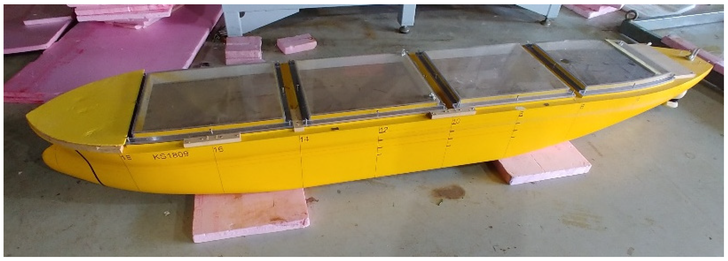
2.1. Experimental Model
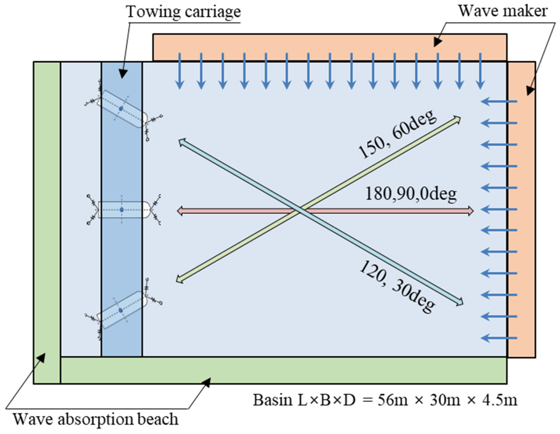
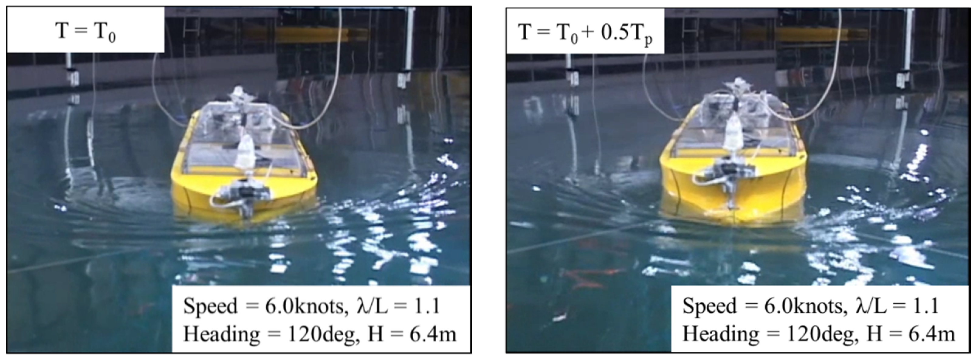
2.2. Test Conditions
2.3. Measurement
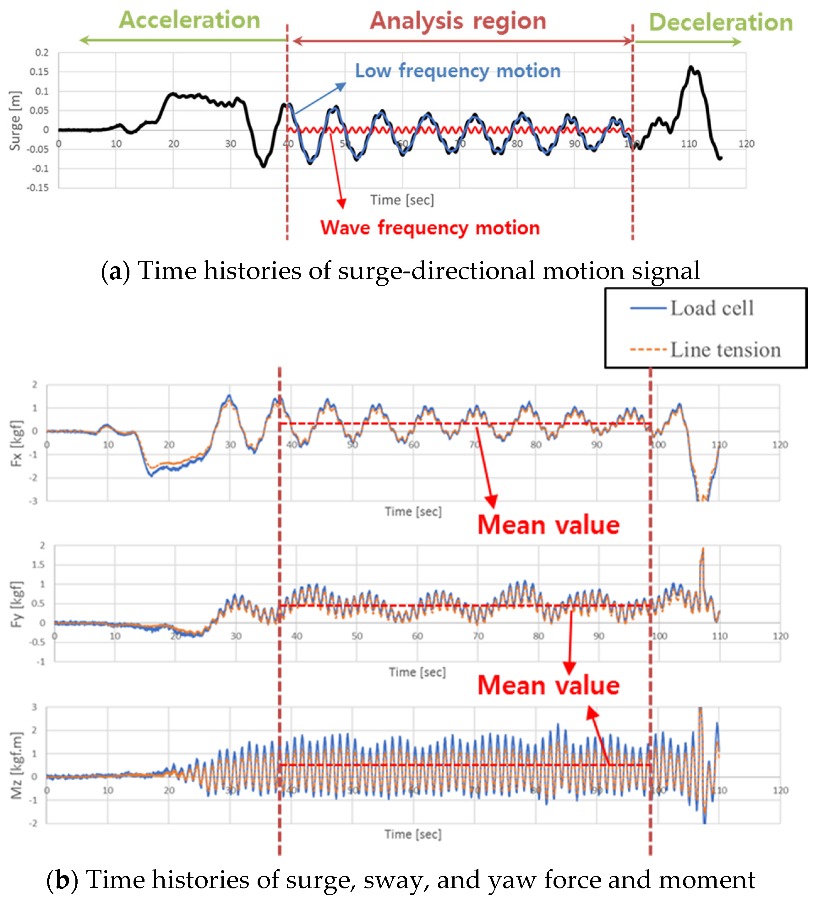
2.4. Data Analysis
3. Numerical Method
4. Results
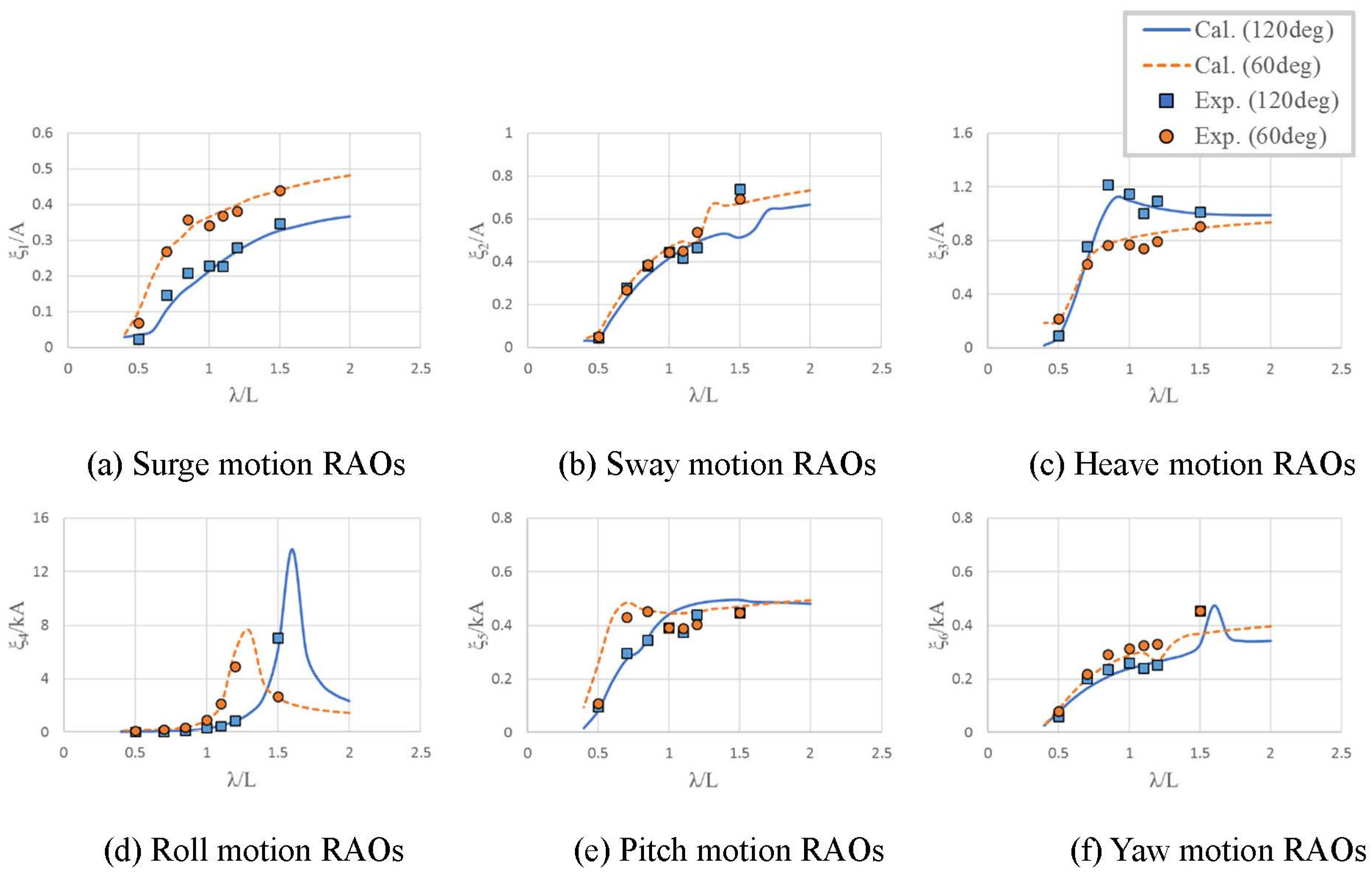
4.1. Motion RAOs
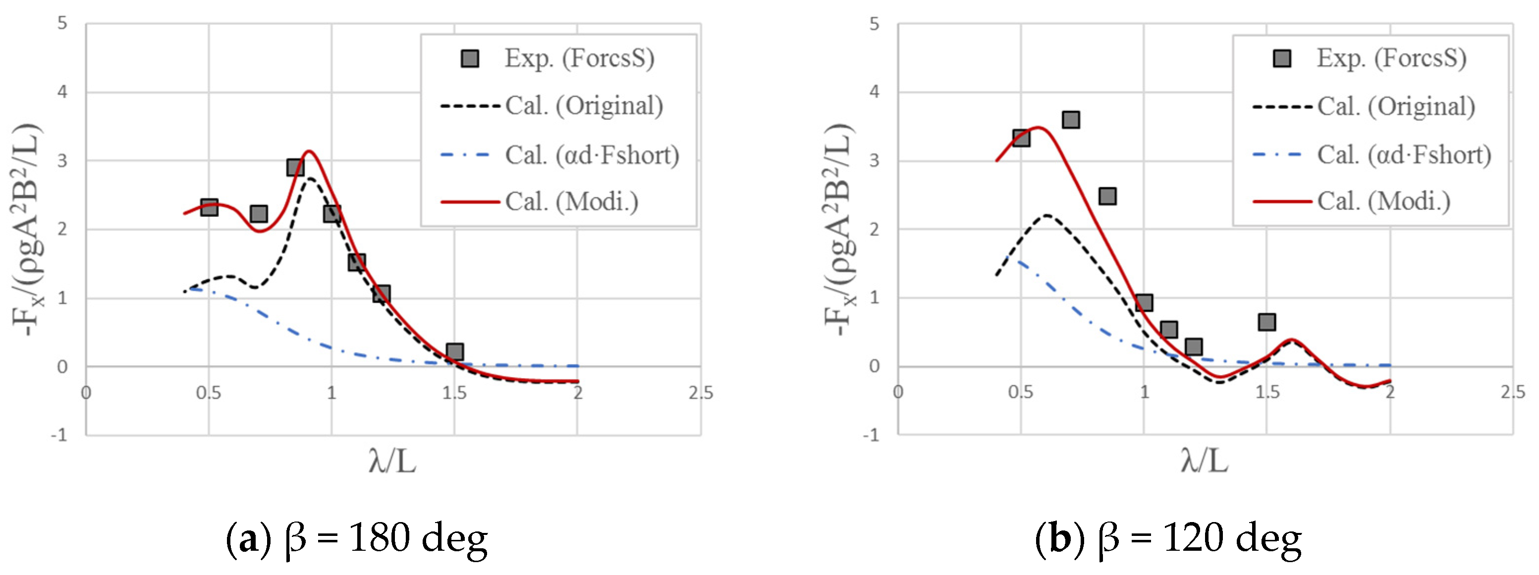
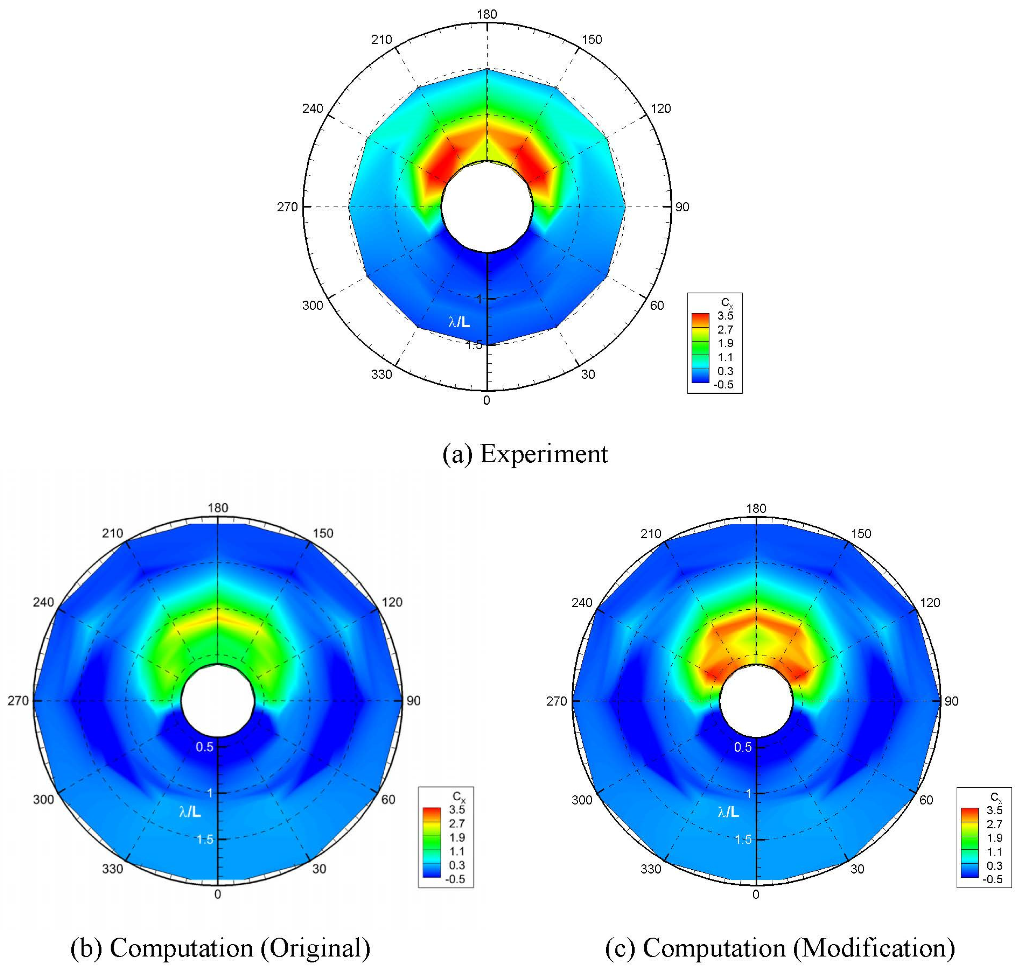
4.2. Surge Wave Drift Force (Added Resistance)
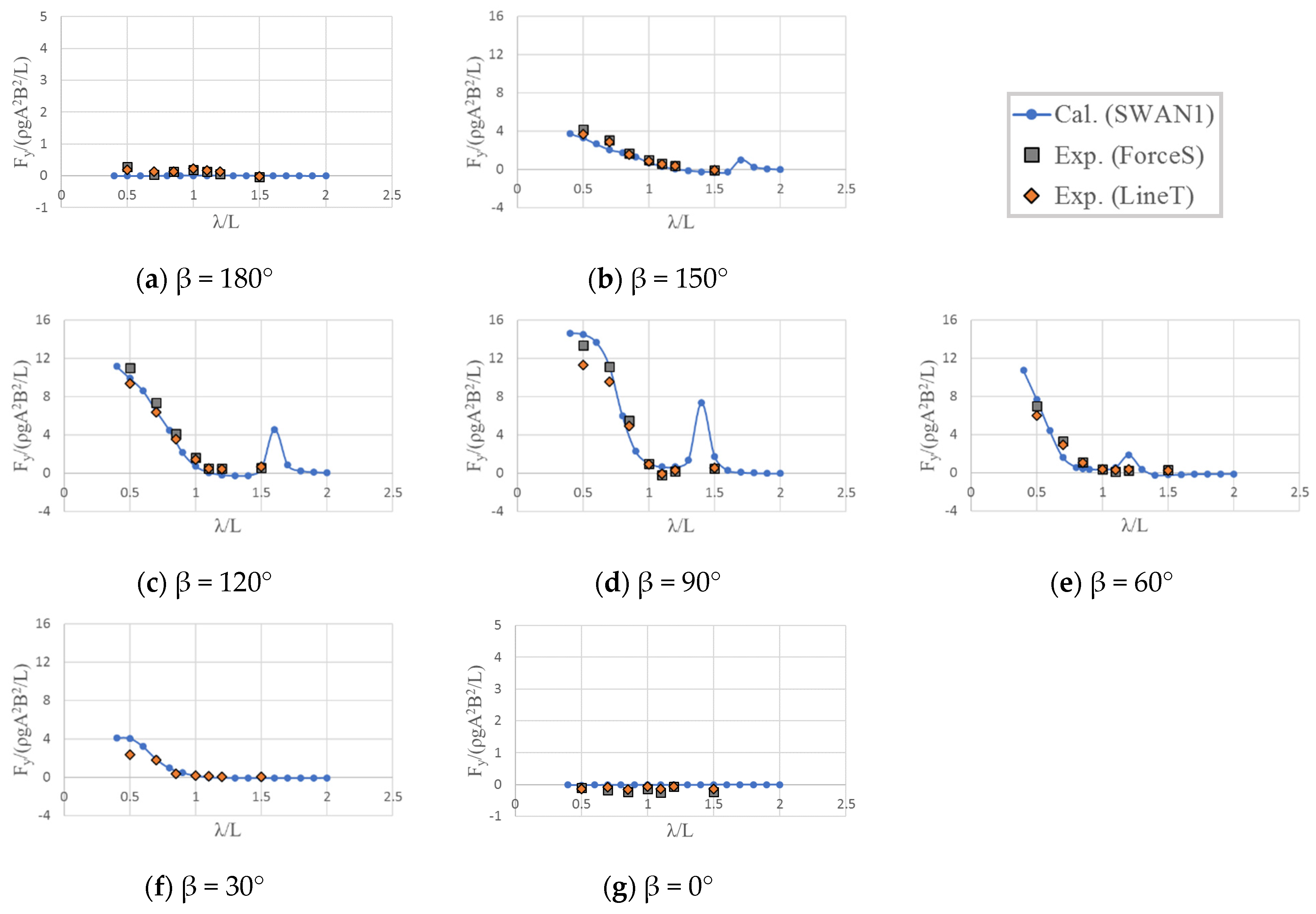
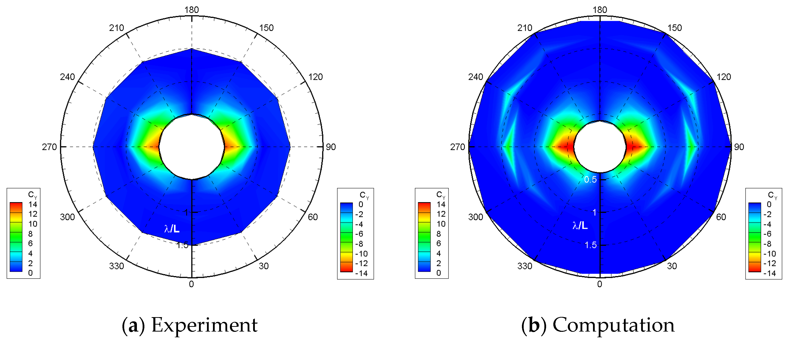
4.3. Sway Wave Drift Force
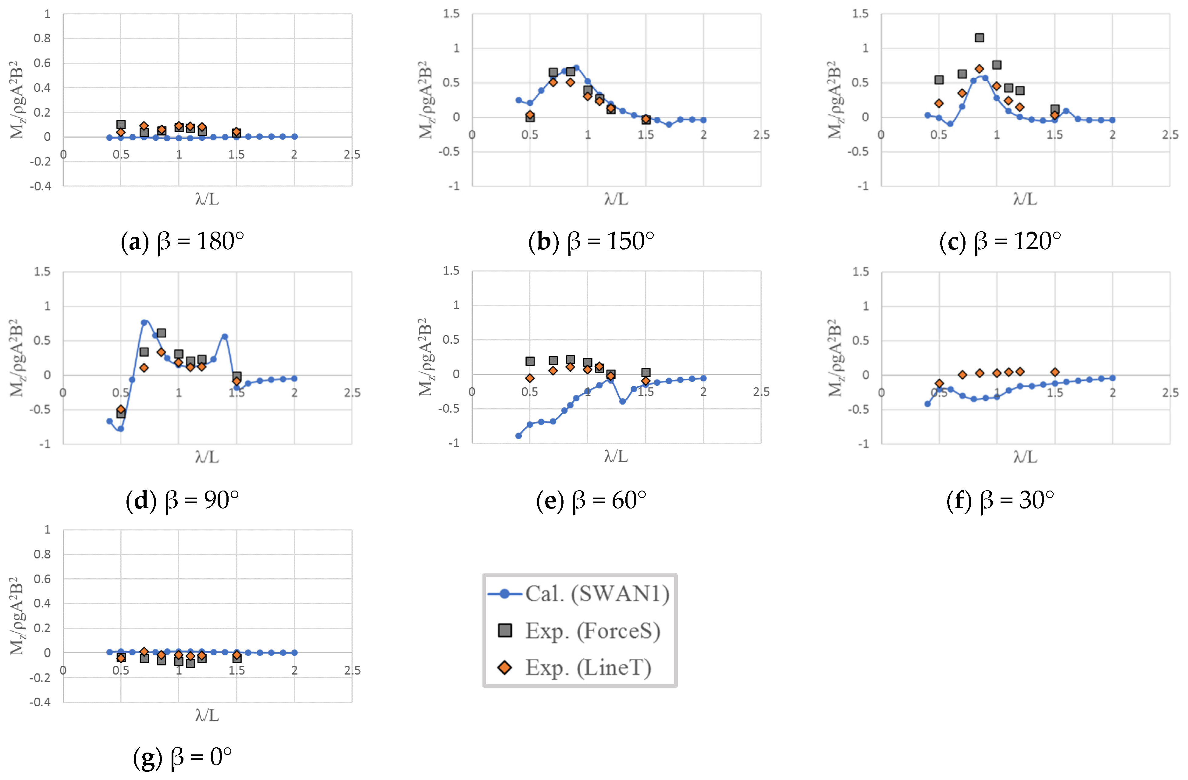
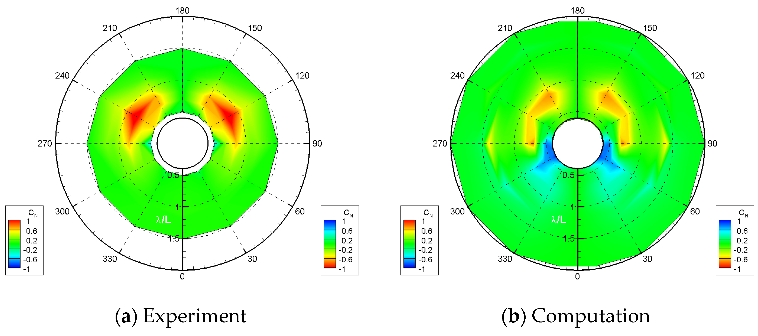
4.4. Yaw Wave Drift Moment
5. Conclusions
- −
- A measurement system for the wave drift force on a ship sailing with forward speed was successfully designed and developed. An indirect method using tensiometers of soft spring had a relatively significant loss of the measuring value due to the friction of the pulley; therefore, a direct method using force sensors is suitable for accurate measurement of the wave drift force and moment;
- −
- Through a series of model tests, the validation data for the wave drift force are obtained. It was confirmed that potential based computation method could predict the 6-DOF motion with high reliability, and the overall tendency of the wave drift force and moment calculated using the numerical method was very similar to experimental data;
- −
- In the case of the surge drift force calculated by the potential based numerical method, the overall trends were similar, but the magnitude near the short wavelength (λ/L < 0.8) was smaller than the experimental value. These discrepancies could be improved using the NMRI method. A negative value of the surge drift force was found near the stern quartering sea in the experimental data as well as the computational results, which suggests that the ship’s total resistance could be decreased when meeting the stern quartering sea;
- −
- The sway wave drift force calculated by the numerical method was almost the same as the experimental value, whereas the yaw wave drift moment showed discrepancies. This meant that the total summations of the second-order pressure on the ship’s side surface were similar, but the pressure distribution was different. Notably, the pressure gradient was not adequately applied in the numerical analysis owing to the flow separation in the stern area. Therefore, it is recommended to carefully use the yaw drift moment calculated by the numerical computation based on the potential theory.
Author Contributions
Funding
Institutional Review Board Statement
Informed Consent Statement
Acknowledgments
Conflicts of Interest
References
- Marine Environment Protection Committee. 2013 Guidelines for Calculation of Reference Lines for Use with the Energy Efficiency Design Index (EEDI); MEPC, 2013. Available online: https://scholar.google.com.hk/scholar?cluster=4054065354720390642&hl=zh-CN&as_sdt=0,5 (accessed on 28 January 2021).
- Marine Environment Protection Committee. Interim Guidelines for Degerming Minimum Propulsion Power to Maintain the Manoeuvrability of Ships in Adverse Conditions; MEPC, 2013. Available online: https://www.researchgate.net/publication/315642605_2013_INTERIM_GUIDELINES_FOR_DETERMING_MINIMUM_PROPULSION_POWER_TO_MAINTAIN_THE_MANOEUVRABILITY_OF_SHIPS_IN_ADVERSE_CONDITIONS (accessed on 28 January 2021).
- Yasukawa, H. Simulations of ship maneuvering in waves (1st report: Turning motion). J. Jpn. Soc. Nav. Archit. Ocean. Eng. 2006, 4, 127–136. [Google Scholar] [CrossRef] [Green Version]
- Yasukawa, H.; Zaky, M.; Yonemasu, I.; Miyake, R. Effect of engine output on maneuverability of a VLCC in Still water and adverse weather conditions. J. Mar. Sci. Technol. 2017, 22, 574–586. [Google Scholar] [CrossRef] [Green Version]
- Sprenger, F.; Fathi, D. Report on Model Tests at MARINTEK (Trondheim Norway); SHOPERA: Trondheim, Norway, 2015. [Google Scholar]
- Maron, A. Report on Model Tests at CEHIPAR (Madrid Spain); SHOPERA: Madrid, Spain, 2015. [Google Scholar]
- Kim, D.J.; Yun, K.; Park, J.-Y.; Yeo, D.J.; Kim, Y.G. Experimental investigation on turning characteristics of KVLCC2 tanker in regular waves. Ocean Eng. 2019, 175, 197–206. [Google Scholar] [CrossRef]
- Seo, M.-G.; Nam, B.W.; Kim, Y.-G. Numerical evaluation of ship turning performance in regular and irregular waves. J. Offshore Mech. Archit. Eng. 2019, 142, 1–31. [Google Scholar] [CrossRef]
- Maruo, H. The drift of a body floating on waves. J. Ship Res. 1960, 4, 1–10. [Google Scholar]
- Newman, J.N. The drift force and moment on ships in waves. J. Ship Res. 1967, 11, 51–60. [Google Scholar] [CrossRef]
- Faltinsen, O.M.; Minsaas, K.J.; Liapis, N.; Skjørdal, S.O. Prediction of resistance and propulsion of a ship in a seaway. In Proceedings of the 13th Symposium on Naval Hydrodynamics, Tokyo, Japan, 6–8 October 1980; pp. 505–529. [Google Scholar]
- Bunnik, T. Seakeeping Calculations for Ships, Taking into Account the Non-Linear Steady Waves. Ph.D. Thesis, Delft University of Technology, Delft, The Netherlands, 22 November 1999. [Google Scholar]
- Zhang, S.; Weems, K.M.; Lin, W.-M. Investigation of the horizontal drifting effects on ships with forward speed. In Proceedings of the 28th International Conference on Ocean, Offshore and Arctic Engineering, Honolulu, HI, USA, 31 May–5 June 2018; pp. 433–440. [Google Scholar]
- Joncquez, S.A.G. Second-Order Forces and Moments Acting on Ships in Waves. Ph.D. Thesis, Technical University of Denmark, Copenhagen, Denmark, 2009. [Google Scholar]
- Kim, K.H.; Seo, M.G.; Kim, Y. Numerical analysis on added resistance of ships. Int. J. Offshore Polar Eng. 2012, 21, 21–29. [Google Scholar]
- Lee, J.-H.; Kim, Y. Study on added resistance of a ship under parametric roll motion. Ocean Eng. 2017, 144, 1–13. [Google Scholar] [CrossRef]
- Seo, M.-G.; Kim, Y.; Park, D.-M. Effect of internal sloshing on added resistance of ship. J. Hydrodyn. 2017, 29, 13–26. [Google Scholar] [CrossRef]
- Park, D.-M.; Kim, Y.; Seo, M.-G.; Lee, J. Study on added resistance of a tanker in head waves at different drafts. Ocean Eng. 2016, 111, 569–581. [Google Scholar] [CrossRef] [Green Version]
- Park, D.-M.; Kim, J.-H.; Kim, Y. Numerical study of added resistance of flexible ship. J. Fluids Struct. 2019, 85, 199–219. [Google Scholar] [CrossRef]
- Seo, M.-G.; Yang, K.-K.; Park, D.-M.; Kim, Y. Numerical analysis of added resistance on ships in short waves. Ocean Eng. 2014, 87, 97–110. [Google Scholar] [CrossRef]
- Martić, I.; Degiuli, N.; Farkas, A.; Gospić, I. Evaluation of the effect of container ship characteristics on added resistance in waves. J. Mar. Sci. Eng. 2020, 8, 696. [Google Scholar] [CrossRef]
- Kuroda, M.; Tsujimoto, M.; Fujiwara, T.; Ohmatsu, S.; Takagi, K. Investigation on components of added resistance in short waves. J. Jpn. Soc. Nav. Archit. Ocean Eng. 2008, 8, 171–176. [Google Scholar] [CrossRef] [Green Version]
- Tsujimoto, M.; Shibata, K.; Kuroda, M.; Takagi, K. A practical correction method for added resistance in waves. J. Jpn. Soc. Nav. Archit. Ocean Eng. 2008, 8, 177–184. [Google Scholar] [CrossRef] [Green Version]
- Yang, K.-K.; Kashiwagi, M.; Kim, Y. Numerical study on ship-generated unsteady waves based on a cartesian-grid method. J. Hydrodyn. 2020, 32, 953–968. [Google Scholar] [CrossRef]
- Kashiwagi, M. Hydrodynamic study on added resistance by means of unsteady wave analysis. J. Jpn. Soc. Nav. Archit. Ocean Eng. 2013, 57. [Google Scholar] [CrossRef]
- Liu, S.; Papanikolaou, A. Regression analysis of experimental data for added resistance in waves of arbitrary heading and development of a semi-empirical formula. Ocean Eng. 2020, 206, 107357. [Google Scholar] [CrossRef]
- Jinkine, V.; Ferdinande, V. A method for predicting the added resistance of fast cargo ships in head waves. Int. Shipbuild. Prog. 1974, 21, 149–167. [Google Scholar] [CrossRef]
- Storm-Tejsen, J.; Yeh, H.Y.H.; Moran, D.D. Added resistance in waves. Trans. Soc. Nav. Archit. Mar. Eng. 1973, 81, 250–279. [Google Scholar]
- Fujii, H.; Takahashi, T. Experimental study on the resistance increase of a large full ship in regular oblique waves. In Proceedings of the 14th International Towing Tank Conference (ITTC1975), Ottawa, ON, Canada, 11 September 1975; pp. 351–360. [Google Scholar]
- Nakamura, S.; Naito, S. Propulsive performance of containership in waves. J. Soc. Nav. Archit. Jpn. 1977, 15, 24–48. [Google Scholar]
- Guo, B.J.; Steen, S. Evaluation of added resistance of KVLCC2 in short waves. J. Hydrodyn. 2011, 23, 709–722. [Google Scholar] [CrossRef]
- Sadat-Hosseini, H.; Wu, P.-C.; Carrica, P.M.; Kim, H.; Toda, Y.; Stern, F. CFD verification and validation of added resistance and motions of KVLCC2 with fixed and free surge in short and long head waves. Ocean Eng. 2013, 59, 240–273. [Google Scholar] [CrossRef]
- Park, D.-M.; Lee, J.; Kim, Y. Uncertainty analysis for added resistance experiment of KVLCC2 ship. Ocean Eng. 2015, 95, 143–156. [Google Scholar] [CrossRef]
- Lee, J.; Park, D.-M.; Kim, Y. Experimental investigation on the added resistance of modified KVLCC2 hull forms with different bow shapes. Proc. Inst. Mech. Eng. Part M J. Eng. Marit. Environ. 2017, 231, 395–410. [Google Scholar] [CrossRef]
- Joncquez, S.A.G. Comparison Results from S-OMEGA and from AEGIR; FORCE Technology: Brøndby, Denmark, 2011. [Google Scholar]
- Simonsen, C.D.; Otzen, J.F.; Nielsen, C.; Stern, F. CFD prediction of added resistance of the KCS in regular head and oblique waves. In Proceedings of the 30th Symposium on Naval Hydrodynamics, Hobart, Tasmania, Australia, 2–7 November 2014. [Google Scholar]
- Park, D.M.; Lee, J.H.; Jung, Y.W.; Lee, J.; Kim, Y. Comparison of added resistance in oblique seas by numerical analysis and experimental measurement. In Proceedings of the 28th International Ocean and Polar Engineering Conference, Sapporo, Japan, 10–15 June 2018. [Google Scholar]
- Nakos, D.E. Ship Wave Patterns and Motions by a Three Dimensional Rankine Panel Method. Ph.D. Thesis, Massachusetts Institute of Technology, Cambridge, MA, USA, June 1990. [Google Scholar]
- Seo, M.-G.; Park, D.-M.; Yang, K.-K.; Kim, Y. Comparative study on computation of ship added resistance in waves. Ocean Eng. 2013, 73, 1–15. [Google Scholar] [CrossRef]


| Item | Unit | Proto | Model |
|---|---|---|---|
| Scale ratio | [-] | 1 | 1/100 |
| Length | [m] | 320.0 | 3.200 |
| Breadth | [m] | 58.0 | 0.580 |
| Draft | [m] | 20.8 | 0.208 |
| Displacement volume | [m3] | 312,622.0 | 0.313 |
| Longitudinal center of gravity from midship | [m] | 11.1 | 0.111 |
| Metacentric height | [m] | 5.8 | 0.058 |
| Longitudinal gyration (kyy/L) | [-] | 0.239 | 0.239 |
| Roll period | [sec] | 17.3 | 1.730 |
| Item | Case | # of Case |
|---|---|---|
| Wave direction, β [deg] | 180, 150, 120, 90, 60, 30, 0 | 7 |
| Wave length (λ/L) | 0.5, 0.7, 0.85, 1.0, 1.1, 1.2, 1.5 | 7 |
| Wave height, h [m] | 6.4 (H/L = 1/50) | 1 |
| Ship speed [knots] | 15.5, 6.0 | 2 |
| Total Cases | 98 | |
| Measurement Item | Sensor | # of Channels |
|---|---|---|
| 6-DOF motions | RODYM | 6 |
| Wave elevation | Capacitance-type wave probe | 2 |
| Relative wave motion | Capacitance-type wave probe | 3 |
| Mooring line tension | 1-axis load cell | 4 |
| Global force | 2-axis load cell | 4 |
| Total channels | 19 | |
Publisher’s Note: MDPI stays neutral with regard to jurisdictional claims in published maps and institutional affiliations. |
© 2021 by the authors. Licensee MDPI, Basel, Switzerland. This article is an open access article distributed under the terms and conditions of the Creative Commons Attribution (CC BY) license (http://creativecommons.org/licenses/by/4.0/).
Share and Cite
Seo, M.G.; Ha, Y.J.; Nam, B.W.; Kim, Y. Experimental and Numerical Analysis of Wave Drift Force on KVLCC2 Moving in Oblique Waves. J. Mar. Sci. Eng. 2021, 9, 136. https://doi.org/10.3390/jmse9020136
Seo MG, Ha YJ, Nam BW, Kim Y. Experimental and Numerical Analysis of Wave Drift Force on KVLCC2 Moving in Oblique Waves. Journal of Marine Science and Engineering. 2021; 9(2):136. https://doi.org/10.3390/jmse9020136
Chicago/Turabian StyleSeo, Min Guk, Yoon Jin Ha, Bo Woo Nam, and Yeongyu Kim. 2021. "Experimental and Numerical Analysis of Wave Drift Force on KVLCC2 Moving in Oblique Waves" Journal of Marine Science and Engineering 9, no. 2: 136. https://doi.org/10.3390/jmse9020136