Feasibility Study for the Extraction of Wave Energy along the Coast of Ensenada, Baja California, Mexico

Abstract

Mexico is one of the countries with the highest emissions of greenhouse gases. In order to reduce the emission of contaminants due to fossil fuels, the state of Baja California has recently launched several research projects for the optimization of facilities for the exploitation of renewable sources, and in particular wave energy. In this work a first-level feasibility study of energy extraction from wave motion is presented for the Ensenada coast, along a complex distance of more than 200 km. The methodology proposed provides good spatial and temporal resolution for wave heights and periods calculation and consequently for the wave power. The methodology is based on the application of the coupled Simulated Waves Nearshore and Advanced Circulation (SWAN + ADCIRC) model for generation, propagation and dissipation of waves. To take into account the meteorological variability within a 21-year dataset, the Typical Meteorological Year method was applied. Results show that overall, the most persistent energy potential during the year is >2 kW/m, with peaks of 5 and 10 kW/m during few months. Given the theoretical energy potential calculated, the Ensenada coast could produce hundreds of GWh per year. The proposed methodology can be applied for the exploration of other coasts with energy potential.

1. Introduction

Research and inversion in marine energy, combined with other renewable energy sources, such as solar, wind, and tidal, can help reduce environmental problems (e.g., pollution and CO${}_2$ production), as well as overcome and compensate for the progressive reduction of fossil fuels. Pollution and the production of energy through fossil fuels are closely linked to each other. Oil, coal and natural gas are the main causes of greenhouse gas emissions worldwide, with a clear effect on the temperature increase associated with climate change, and many other negative consequences on the environment which are now recognized worldwide. Moreover, even if fossil fuels are still available at the moment, they constitute a finite source of energy, and therefore represent a source of conflict. Nowadays, for many countries around the world, reducing their dependence on fossil fuels has become an important goal of energy policies. The Danish Commission on Climate Change, for example, in 2010 presented a proposal for activities to make the country independent of fossil fuels by 2050 [1]. Of course, the key to achieving this ambitious goal is through the use of renewable energy. The assessment of wave energy resource has been extensively studied through the description of sea states, how energy yield is estimated from wave data, the variability of energy yield and the methods for the estimation of influence of extreme wave conditions [2]. Many projects have been developed with the aim of providing and standardizing details and procedures for extracting energy from waves. For example, the EquiMar project [3], founded by the European Commission under the seventh Framework Program, was created with the aim of accelerating the production rate of the different models of devices for extracting energy from waves. In addition, the International Electrotechnical Commission has established a specific protocol to analyze the sites potentially suitable for the installation of Wave Energy Converters [4]. Finally, a recent review on wave energy resource assessment, based on the most recent resource characterizations, performs a deep analysis and description of the formulations and energy metrics and shows the limitations and potential of the different methods currently in use for energy extraction on the bases of results obtained in the most energetic locations around the world [5].

It is estimated that globally, the energy potential that can be extracted from the marine environment (from the exploitation of currents, tides, waves, saline and thermal gradient) is, on average, of the order of 2.7 (−70) TW. If we compare this value with the global energy consumption data from the International Energy Agency (IEA), updated to July 2020 [6], it can be seen that marine energy constitutes a resource that could cover global electricity needs.

Mexico is one of the 20 countries with the highest emissions of greenhouse gases, and given its high contribution to climate change, in recent years it made a commitment to reducing greenhouse gas pollution, for example through the General Climate Change Law of 2012, ratified and signed in the Paris Agreement (2015–2016). Furthermore, in the document of the National Climate Change Strategy published in 2013, Mexico proposes objectives, strategies and priority actions, with a vision of up to 40 years, on the subject of climate change. In the document on the Renewable Energy Perspective (2017–2030) [7], Mexico is committed to reducing the consumption of fossil fuels and estimates that 37.7% of the national electricity will be produced by clean energy for 2050. In this context, the state of Baja California represents a unique case of compromise for the optimization of facilities for the energy production and the exploitation of renewable energies potential, as reported in the Institute of the Americas’ Energy Outlook 2020–2025 [8]. Since 2014, the Center for Scientific Research and Higher Education of Ensenada (CICESE), has been developing studies aimed at exploiting wave energy in Baja California, particularly along the coast of Ensenada, and is creating detailed wave data maps to provide a useful database in the renewable energy sector. Finally, a recent collaboration between the CICESE and the University of Manchester, has launched a study for the development and optimization of a prototype for the conversion of wave energy into electrical energy, to be installed along the coast of Ensenada (https://mexiconewsdaily.com/news/wave-power-system-6-times-more-efficient/, accessed on 10 October 2020). According to the news reported by newspapers (no scientific publication was found on the subject), based on wave characteristics in the area, the designed device could generate up to 2 MW and provide electricity to 100,000 homes.

A recent study [9] provides a theoretical estimation of available power from waves, ocean currents, thermal gradients and salinity, along the coast of Mexico using the ERA-Interim public wave field database, from which 10 years of daily data with a spatial resolution of 1/8 × 1/8 degrees are extracted. According to this study, the greatest availability of wave energy is found in the Pacific Ocean. Here, the energy is calculated in the order of 2–10 kW/m and is found constant during 50% of the year. In addition, the recommended places for extracting waves energy are found in the coasts of Baja California, Southern Baja California, Jalisco, Colima, Michoacán, Guerrero and Oaxaca. The same article underlines that specific high-resolution studies particularly aimed at the extractable energy potential near the coast of Mexico, have not yet been carried out as of now. For this reason, a methodology for a first-level assessment of expected efficiency of wave-power plant along the coast of Ensenada, based on typical meteorological conditions is proposed. The present work is focused on the estimation of the efficiency of a wave-power plant, for which it is necessary to run a wave generation and propagation modeling for the study area. Wave-generation simulations are performed with the Simulated Waves Nearshore and Advanced Circulation (SWAN + ADCIRC) model [10]. The modeling process requires input meteorological variables (the two horizontal components of wind speed, and the surface pressure) on a computational grid. In order to grasp the variability of meteorological conditions and to avoid the performance of a large number of wave-generation simulations, the Typical Meteorological Year (from now on, TMY) is identified for the study area, on the basis of the original method of Finkelstein and Schafer [11] and using a 21 years wind data set with 0.25 degrees resolution. Having identified the TMY for the area, the expected energy can be estimated for one representative run. Simulation results, for significant wave heights and peak periods, are used for the calculation of the wave power in a representative number of nodes within the computational grid, at a distance of about 100 km from the coast. Furthermore, the energy availability is calculated for each month of the TMY with the corresponding percentage of availability during every single month and throughout the year, for different energy thresholds.

The remainder of this paper is organized as follows. Section 2 presents Materials and Methods used, including a brief description of the study area, the methodology applied for the Typical Meteorological Year selection, the description of the SWAN + ADCIRC model and its application to the study area, and finally, the calculation of the energy potential. Results for wave characteristics and calculated wave energy are shown in Section 3. A discussion of the implications of the findings encountered is presented in Section 4.

2. Materials and Methods

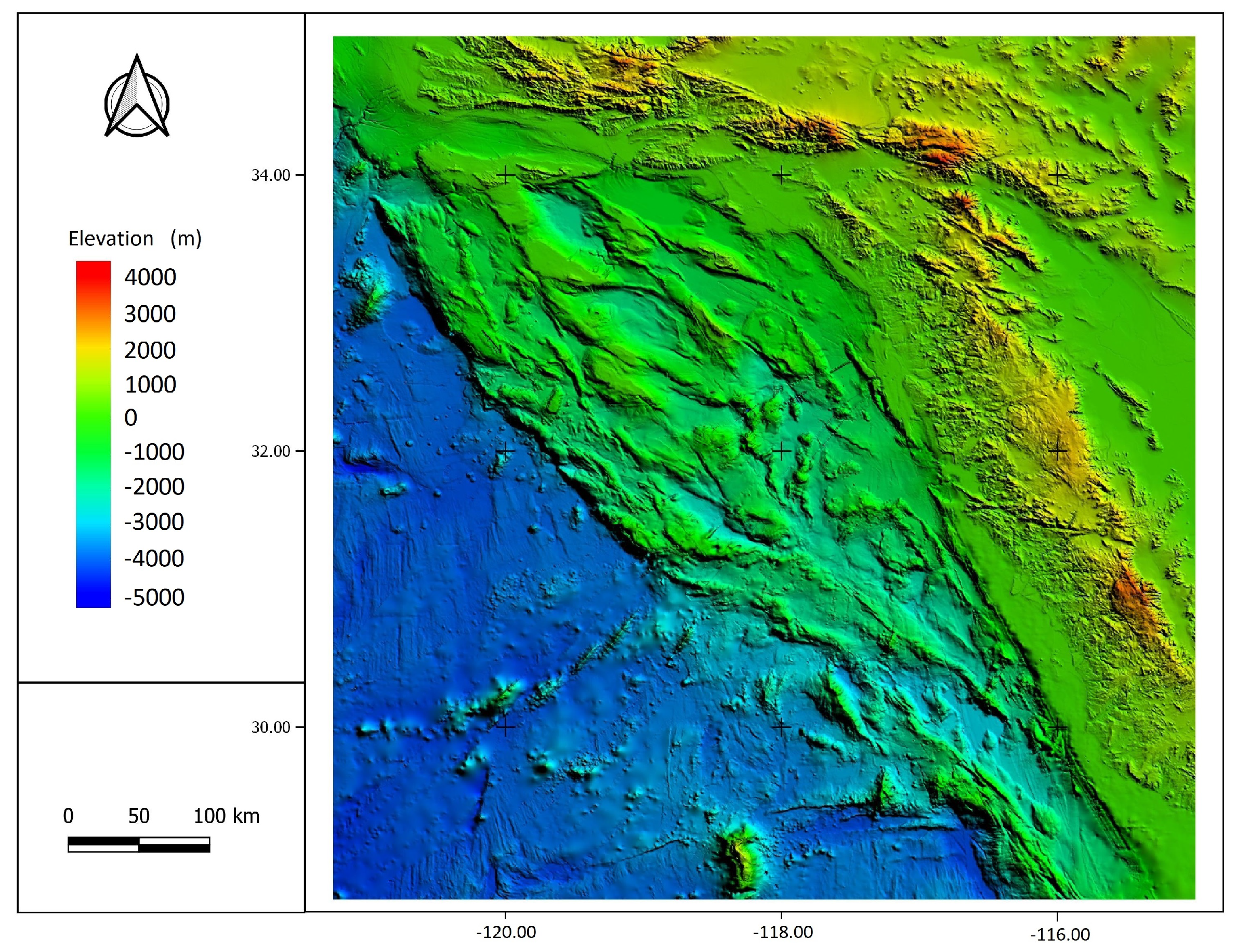
2.1. Characteristics of the Study Area

With the aim of carrying out an assessment of waves as an energy resource in a specific region, it is important to analyze specific factors of the area, such as the climate variability and socio-economic aspects. The city of Ensenada is located within the North Pacific maritime region (Figure 1).

Overall, the municipality of Ensenada occupies a territory of 19,538 km${}^2$, with a population of more than 500,000 inhabitants. The port of Ensenada is located within the Todos Santos bay, which has an approximate area of 180 km${}^2$. This bay is characterized by the presence of an underwater canyon to the southeast that gives the bathymetry the shape of a river valley with depths that change abruptly from 50 m to 390 m. Figure 2, shows the bathymetry of the study area, which is irregular and has numerous islands and islets, in addition it presents abrupt variations in the slopes. The seabed has maximum elevations of 700 m in the islets and depths of up to approximately 4250 m at distances of 360 km from the coastline.

The marine circulation within the Ensenada coast is dominated by the prevailing wind pattern from NW [12]. During spring and summer the predominant wind blows from the NW, with magnitude of 9–18 km/h; in the winter, the passage of winter storms, associated with cold fronts from the Gulf of Alaska, can lead to strong winds from SW (<90 km/h). Within the Todos Santos bay, wave heights greater than 3 m have been registered, however in the mouth and the bay of the Ensenada port, maximum heights between 1.5 and 2 m are recognized [12]. A statistical analysis of the waves in the zone [13], show that the significant wave height follows a seasonal variation, with a maximum significant wave height of 2.1 m in winter and a minimum of 0.4 m in summer. The maximum and minimum peak period values are found to be 5 and 18 s, respectively.

According to [14], there are some aspects to be considered for the definition of sites for the use of ocean energy, which also include external factors such as navigation activities, fishing, recreation, underwater research, military activities. For this reason, it is important to mention that the coast of Ensenada is characterized by the presence of a protected natural area, El Estero de Punta Banda, which was designated, in 1995, as an ecological preservation area. In addition, the port of Ensenada has an anchorage area for merchant and cruise ships, as well as nearby areas for commercial and sport fishing. To take these aspects into consideration, and in line with the maximum distances reached by power cables [15], in this work the analysis of wave characteristics and the consequent potential energy calculation, is performed at a distance of approximately 100 km from the coast line.

2.2. Typical Meteorological Year

The Typical Meteorological Year (from now on, TMY) consists of 12 typical meteorological months that best represent median weather conditions over a multilayer period. A TMY dataset condenses into one year the most usual meteorological conditions. This method has been widely used in computer simulations of building energy [16,17,18] and solar energy conversion systems [19,20,21] since it has been proved to have strong practical validity and provides a general tool to identify suitable areas based on typical meteorological conditions in a cheap and quick manner.

In the present study the TMY has been calculated based on the original method of [11], adapted to the calculation of a TMY in terms of wind speed and direction as previously realized in [22], with the addition that, here, atmospheric pressure at the sea surface is also considered. It is important to note that, because the TMY represents typical atmospheric conditions, it minimizes the difference with the long-term time series. Thus, it does not take into account the extreme meteorological conditions that can occur in the study area (i.e., hurricanes, tropical storms, etc.), which strongly differ from long-term time series and are therefore never selected.

The methodology proposed in this work is based on a 21 years (1998–2018) ERA5 global reanalysis dataset [23] provided by the EMCWF (European Centre for Medium-Range Weather Forecasts). The choice of this dataset is based on the results of a recent study by [24], which compares five global reanalysis database with observations. Ramon et al. (2019) identifies ERA5 as the one that best represents the wind speed features and in particular near-surface winds. The meteorological variables at stake (surface pressure, horizontal and vertical velocity components at 10 m) were downloaded for all points of the 0.25 degrees resolution grid in the study area, corresponding to approximately 25 km (Figure 3a). Wind roses show the direction towards with the wind blows.

The selection of the TMY was made on the basis of the following procedure.

• For each variable, the original data, available in the four-times-daily format, was averaged into one daily value.
• For each month and variable (i.e., wind speed, direction and surface pressure), the long-term and short-term Cumulative Distribution Functions (CDF) are calculated. By short-term we refer to the time series for the specific month (e.g., 1998), while by long-term we refer to the time series of all concatenated Januaries in the period 1998–2018.
• For each month and variable, the Filkestein–Schafer factor (FS) (defined in [11]) for the month is calculated as a function of the absolute difference between long and short-term CDFs. The sum of such absolute differences over the CDF bins is then normalized by the number of bins.
• The final FS for the month is estimated as a weighted sum of the FSs calculated for each variable, using equal weights.
• The five years with minimum FS factor are selected as month’s TMY.
• For each candidate month, the Root Mean Square Difference (RMSD) between long and short-term data is calculated.
• The year having minimum RMSD is the representative year for the month at stake.

This procedure identifies the 12 months that constitute the TMY in each point of the considered spatial grid. In order to compare the results for selected points in the domain, wind roses were produced both for the TMY and for the long-term dataset (Figure 3b,c, respectively). The analysis of spatial variability of the TMY wind roses in the study area shows that wind speed is lower close to the coast and in the mainland. Wind speed and direction look very similar in the oceanic part of the domain, where there is a clear predominance of winds blowing towards the southeast (confirming the observations of [12]), while points in the mainland show different patterns. The visual comparison between the TMY and long-term wind roses at selected points shows very similar trends (Figure 3b,c) confirming the TMY representativity for the purpose of this study. Similarly to [22], it is thus possible to run the wave propagation model for one, representative year and ensure the long-term representativity of the results and reducing the computational time. Since the best meteorological inputs to initialize the wave generation and propagation model should be representative of the meteorological conditions at approximately 100 km from the coast, the point that better fulfills these conditions is point P13 (Figure 3a, highlighted). The selected TMY for this point is shown in

Table 1. Selected typical meteorological year.

Month	1	2	3	4	5	6
Year	2004	2009	2009	2003	1999	2007
Month	7	8	9	10	11	12
Year	2010	2006	2003	2014	2003	2016

. The identified TMYs for all points in Figure 3a are included in a table as Supplementary Material (SM-1: 1. Supplementary Tables). The wind roses and wind speed and direction histograms for the points for which wind roses are shown in Figure 3b,c are also attached as Supplementary Material (SM-1: 2. Supplementary Figures).

In order to check how winds are expected to change in the future in the study area, we compared the wind roses of the long-term pressure and wind data series of two time periods: 1998–2020 (similar to the one used to estimate the TMY in this study) and 2071–2080 decade, for which climatic projections are available within the CESM1 CAM5 large ensemble [25]. This dataset, based on the RCP8.5 forcing scenario (http://www.cesm.ucar.edu/projects/community-projects/LENS/, accessed on 10 October 2020), contains atmosphere 6-hourly post-processed data (pressure and wind speed horizontal components) at different sigma levels, the lower being approximately 60 m over sea level. Figure 4 shows the comparison between the long-term wind roses for the two time periods considered. The plot is produced for point P13 at 100 m height (left) and in the proximity of point P13 at approximately 60 m height (right) for the present and future time periods, respectively.

Figure 4 shows that the wind patterns are not expected to change substantially in the future according to the considered climate projections. The TMYs were also estimated for the two time series shown in Figure 4, and their comparison showed very high similarity. In addition, both TMYs were representative of the respective long-term wind roses. This analysis is based on the comparison of outcomes of two different models (reanalysis and climatic models) at two different heights, and can be thus used only as a base for speculations. However, due to the overall satisfactory agreement with the two time series, we can suppose that the wave energy potential at the end of the current century would be of the same order of magnitude as the one estimated in this work. Further analysis may be performed in future in order to estimate the long-term sustainability of the project in relation to the expected changes in climate and thus in the ocean and atmospheric circulation system.

2.3. The SWAN + ADCIRC Model for Wave Simulations

In order to obtain an accurate depiction of the generation, propagation and dissipation of waves, the SWAN + ADCIRC model [26] has been applied in this work to simulate waves and circulation and their propagation from deep water to nearshore. SWAN is a third-generation nearshore wave model, that simulates wave generation, propagation and dissipation and includes the effects of refraction, shoaling, and blocking in wave propagation and has been extensively used to simulate waves in shallow waters [27,28,29]. Recently the model has been applied to the Canadian Beaufort Sea and storm generated waves through the comparison between in situ buoy observations and numerical simulations [30]. It employees a nesting approach to avoid the overhead associated with grid adaptation at some distance offshore. This problem can be generated by the very variable characteristic spatial scales of the wind waves propagating from deep to shallow waters. It can run on unstructured meshes, being efficient and accurate in the nearshore and deep water. The model predicts the evolution in space and time of the wave action density spectrum according to the action balance equation [31], where no a priori limitations are imposed on the spectral evolution:

$$\frac{\partial N}{\partial t}+{\nabla }_{\overrightarrow{x}}·\left[(\overrightarrow{c_g}+\overrightarrow{U})N\right]+\frac{\partial c_{\theta }N}{\partial \theta }+\frac{\partial c_{\sigma }N}{\partial \sigma }=\frac{S_{tot}}{\sigma }$$

(1)

Being $N(\overrightarrow{x},t,\sigma ,\theta )$ the wave action density spectrum, $\sigma$ the relative frequency and $\theta$ the wave direction. ${\nabla }_{\overrightarrow{x}}$ represents the gradient operator in geographic space, which together with the wave group velocity ($\overrightarrow{c_g}$) and the ambient current vector ($\overrightarrow{U}$), represent the propagation of the wave in space. Refraction and diffraction are represented by the propagation velocity $c_{\theta }$, while $c_{\sigma }$ is the shifting rate due to variations in mean current and depth. The source term $S_{tot}$ encompasses non-linear effects that induce action exchanged between a spectral component in deep and shallow water, other than the wind effect and the bottom friction. Moreover, the source term also accounts for the effects of wave breaking. SWAN runs can be done serial as well as parallel and the output quantities that can be generated include significant wave heights and periods, average wave direction, dissipation, wave-induced force, diffraction parameters, and many more.

On the other hand, ADCIRC is a system of computer programs for solving time-dependent, free surface circulation and transport problems in two and three dimensions. It applies a continuous-Galerkin finite-element method with triangular elements [32,33] to solve the shallow-water equations at a range of scales [34]. The studies in which the model has been applied up to now concern: modeling tidally and wind-driven circulation in coastal waters [35], forecasting hurricane storm surge and flooding [36], riverine modeling for currents and water levels [37], and baroclinic coastal modeling from laboratory scale to field scale [38]. A FORTRAN compiler is available for compiling the model, which can run on any operating system. Among the main features of the model we mention here: two-dimensional depth-integrated (2DDI) and 3D solution capabilities; large domain—localized resolution strategy; runs on single-processor computers and parallel computers using MPI; consistency with the governing equations. Water levels are calculated via the solution of the Generalized Wave Continuity Equation (GWCE):

$$\frac{{\partial }^2\zeta }{\partial t^2}+{\tau }_0\frac{\partial \zeta }{\partial t}+\frac{\partial {\tilde{J}}_x}{\partial x}+\frac{\partial {\tilde{J}}_y}{\partial y}-UH\frac{\partial {\tau }_0}{\partial x}-VH\frac{\partial {\tau }_0}{\partial y}=0$$

(2)

where:

$$\begin{array}{cc}\hfill {\tilde{J}}_x=& -Q_x\frac{\partial U}{\partial x}-Q_y\frac{\partial U}{\partial y}+f{Q}_y-\frac{g}{2}\frac{\partial {\zeta }^2}{\partial x}-gH\frac{\partial }{\partial x}\left[\frac{P_s}{g{\rho }_0}-\alpha \eta \right]\hfill \\ \hfill & +\frac{{\tau }_{sx,wind}+{\tau }_{sx,waves}-{\tau }_{bx}}{{\rho }_0}+(M_x-Dx)+U\frac{\partial \zeta }{\partial t}+{\tau }_0{Q}_x-gH\frac{\partial \zeta }{\partial x}\hfill \end{array}$$

(3)

$$\begin{array}{cc}\hfill {\tilde{J}}_y=& -Q_x\frac{\partial V}{\partial x}-Q_y\frac{\partial V}{\partial y}+f{Q}_y-\frac{g}{2}\frac{\partial {\zeta }^2}{\partial y}-gH\frac{\partial }{\partial y}\left[\frac{P_s}{g{\rho }_0}-\alpha \eta \right]\hfill \\ \hfill & +\frac{{\tau }_{sy,wind}+{\tau }_{sy,waves}-{\tau }_{by}}{{\rho }_0}+(M_y-Dy)+V\frac{\partial \zeta }{\partial t}+{\tau }_0{Q}_y-gH\frac{\partial \zeta }{\partial y}\hfill \end{array}$$

(4)

For $\zeta$ being the water level and U and V the depth-integrated currents in the $x-$ and $y-$ directions; $H=\zeta +h$ the total water depth; h the bathymetric depth; $Q_x=UH$ and $Q_y=VH$ are fluxes per unit width; f is the Coriolis parameter; g is the gravitational acceleration; $P_s$ is the atmospheric pressure at the surface; ${\rho }_0$ is the reference density of the water; $\eta$ is the Newtonian equilibrium tidal potential and $\alpha$ is the effective earth elasticity factor; ${\tau }_{s,wind}$ and ${\tau }_{s,waves}$ are surface stresses due to winds and waves, respectively; ${\tau }_b$ is the bottom stress; M are lateral stress gradients; D are momentum dispersion terms and ${\tau }_0$ is a numerical parameter that optimizes the phase propagation properties.

The coupling of the SWAN wave model and the ADCIRC circulation model is performed by running the two models in the same unstructured mesh, so that it can be applied on a large domain, avoiding the nesting or the overlapping of structured wave meshes. The coupled model is highly scalable and integrates seamlessly the physics from deep ocean to shelf. The performance of the unstructured mesh has been widely examined and the multi-process, multi-scale modeling system has been integrated by utilizing intermodel communication that is intra-core. This performance has been validated through the simulation of hurricanes Catrina (2005), Gustav and Ike (2008) [10].

2.4. Wave Generation and Propagation in the Study Area

Figure 5 shows the delimitation of the computational domain: the red line defines the limit of the coast, while the blue line is the domain limit in the open sea. The study area covers the coastal region of Ensenada and is located within the polygon defined by the points 35.00 N, 28.75 S, −115.00 E, −121.25 W. In order to construct the geometry and the computational mesh, the Digital Elevation Model (DEM) of the Ensenada port was used. The DEM was developed by the General Bathymetric Chart of the Oceans [39], a global terrain model for the ocean and the earth, with arc intervals of 15 s.

The study area was discretized with an unstructured mesh (Figure 5) to obtain levels of spatial resolution in the different zones of the spatial domain. After preliminary tests to evaluate the effect of the mesh size on the results, an unstructured triangular mesh of 19,742 elements was generated, which consists of a total of 10,327 nodes, with a minimum space between nodes of 900 m, near the coastline, and a maximum space of 27,500 m in open sea.

The parameters necessary for forcing the generation and propagation of waves are the tide and the wind field. To insert the tide constituents to the model, the Eastern Pacific Tidal Database (ENPAC15) was used. It includes M2, S2, N2, K2, O1, K1, P1, Q1, M4, M6 constituents and all phases are relative to the Greenwich Meridian. The database was completed in 2015 and was developed using the two-dimensional, depth-integrated form of the ADCIRC model. The ENPAC15 database provides the amplitude and phase for the 37 standard NOS tidal constituents for both elevation and velocity and it has been validated by [40]. In our model, seven main harmonic components have been introduced in the open limit, which include three diurnal astronomical constituents (K1, Q1 and O1) and four semi-diurnal (K2, M2, S2 and N2). These boundary conditions were obtained by interpolating the results of a global finite element oceanic model in each of the open boundary nodes of our model [41]. Regarding the wind field, the horizontal wind components (u, v) plus the atmospheric pressure were used, corresponding to the Typical Meteorological Year (TMY) indicated in the Table 1. As for the TMY calculation, wind data were downloaded from the ERA5 dataset, for the entire extension of the computational domain, with a spatial resolution of 0.25 degrees and a temporal resolution of 60 min.

The analysis of the wave characteristics was carried out on 56 nodes of the computational mesh, selected as “virtual buoys”. The points are distributed along a line parallel to the coast, at a distance of 100 km from it (Figure 6).

2.5. Wave Energy Calculation

Power wave was calculated on the basis of the linear wave theory in deep waters, according to which the theoretical energy potential can be estimated as [42,43,44]:

$$P_{OW}=\frac{W\rho g^2{T}_e{H}_s^2}{64\pi }$$

(5)

where W is the wavefront (assumed to be 1 m), $\rho$ is the seawater density (1025 kg/m${}^3$), $H_s$ is the significant wave height in meters, and $T_e$ is its corresponding energy period, which can be defined as the ratio of the first negative moment of the spectrum to the zeroth moment of the spectrum.

3. Results

3.1. Wave Parameters Analysis

The analysis of the distribution of the most representative wave parameters (significant wave height and peak period) was carried out on the basis of 490,650 records, which represent one record every hour for 365 days, for the 56 “virtual buoys” shown in Figure 6. To verify simulation results, we compared the significant wave height values calculated with the SWAN+ADCIR model with the values present in the ERA5 database (https://cds.climate.copernicus.eu/#!/home, accessed on 23 February 2021). The comparison was made on nodes 1 and 30 (far south and center of our line of virtual buoys), for the twelve months of the TMY. For practical reasons, in Figure 7 we show only the comparison between the calculated values and those of the dataset for the months of January and December.

The figure shows that there is a good correspondence between the calculated $H_s$ values and those of the database, indicating that the model has been applied properly.

The characteristics of the variation of the significant wave heights ($H_s$) throughout the year, were studied using the frequency distribution of this parameter. Figure 8 shows the frequency histogram of the $H_s$ occurrence.

The frequency histogram was described by a Generalized Extreme Values (GEV) probability density function, which provided a mean value of 0.81 m and variance equal to 0.26. It is worth mentioning that the GEV function has been selected as it is the one that best fits the calculated $H_s$ values and therefore provides the best cumulative distribution function. The minimum $H_s$ value (0.1 m) is in agreement with the results of the statistical study by [13] while the maximum value (3.8 m) is slightly higher. The frequency histogram of the peak period $T_p$ is shown in Figure 9.

This distribution can be described by a normal probability density function, which gave a mean value of 5.1 s and variance 1.9. Maximum and minimum $T_p$ values (9.8 s and 1.3 s, respectively) are found to be lower than the ones estimated by [13]. In the aforementioned statistical analysis, the authors used wave values recorded between September 1986 and August 1987, in a station located at the Todos Santos bay. Since the wave period is an extremely variable value that depends on the sea-state, frequently characterized by the coexistence of the local wave system and the background swell, we consider that the one year used in [13] is a statistically short period that can not take into account all the variations to which the wave period is subject, and probably reflects only local effects.

3.2. Wave Energy

To calculate the wave energy, Equation (5) was applied to all 56 nodes selected as virtual buoys. The calculations were performed using the results obtained from the wave height and period simulations, for each hour of the 365 days of the TMY, obtaining a total of more than 490,000 energy potential results. The calculated annual energy average produced by wave motion is 2.4 kW/m. Figure 10 shows how the availability of energy varies during the months of the year.

The energy values shown in the figure correspond to the averages calculated on all nodes. The respective standard deviations are shown in

Table 2. Energy monthly averages and standard deviations calculated on 56 nodes over a total of 490,650 records.

	Average in kW/m	Standard Deviation
January	2.0	4.0
February	3.1	7.2
March	2.9	6.0
April	3.5	3.6
May	4.8	4.9
June	2.5	3.9
July	1.4	1.6
August	1.2	1.0
September	1.7	1.7
October	0.9	1.2
November	1.8	4.5
December	3.2	6.6

.

The months with higher productivity range from December to June, while the months with the lowest productivity are from July to November.

Despite the annual average is slightly greater than 2 kW/m, it is important to note that energy peaks greater than or equal to 5 and 10 kW/m were also calculated, which explains the high standard deviation values calculated in correspondence of some months. For this reason, with the aim of analyzing in more detail the availability of energy in the study area, the calculated values of energy potential were organized into energy thresholds corresponding to: ≥2 kW/m, ≥5 kW/m, ≥10 kW/m. Furthermore, percentages of the days in which the available energy is greater than or equal to each threshold were also calculated, following the methodology proposed by [9].

Table 3. Percentages of days in which the energy is equal to or greater than the energy thresholds: ≥2 kW/m, ≥5 kW/m, ≥10 kW/m. Values are averaged over all nodes and for each month of the TMY.

Month	Energy ≥ 2 kW/m	Energy ≥ 5 kW/m	Energy ≥ 10 kW/m
January	26.3%	8.7%	2.4%
February	33.8%	13.1%	5.8%
March	37.3%	12.0%	4.3%
April	53.2%	27.1%	8.3%
May	55.1%	36.5%	15.5%
June	36.5%	7.4%	5.0%
July	22.3%	4.4%	0.2%
August	16.6%	0.6%	0.0%
September	31.8%	5.5%	0.0%
October	10.9%	2.3%	0.0%
November	17.4%	6.8%	2.6%
December	33.3%	12.7%	6.5%

shows the average of the percentage of days in which energy persists greater than or equal to the thresholds considered.

Overall, energies ≥2 kW/m, are produced during more than 30% of the year. During April and May this production last more than 50% of the months. The months in which this productivity is less persistent are August, October and November. In the remaining months, the energy remains ≥2 kW/m for 30% of the month. Energies greater than 5 kW/m are also obtained, however for less than 20% of the year, except for April and May. Peaks greater than or equal to 10 kW/m are also reached, however for very short periods of the year.

A table containing all calculated energy values for each month on each node is available as Supplementary Material (SM-2). From this table it can be seen that moving away from the virtual buoy 1 towards 56 the production of energy decreases. A closer map of the virtual buoys is visible in the Figure 11.

From node 1 to 30, the percentage of days in which energy remains greater than or equal to 2 kW/m is greater than 50% during the months with the highest productivity, while in the remaining nodes, during the same months, the productivity is less persistent. Looking even more in detail, it can be observed that in nodes from 1 to 8, energy greater than or equal to 2 kW/m is produced during all months of the year with a percentage of days per month that varies between 30 and more than 70%, with October being the month when the energy is least persistent. Energy peaks greater than 5 kW/m are also reached in these nodes, which in April and May remain constant for more than 40% of the month.

4. Discussion

The results of the calculation of energy that can be extracted from the wave motion along the coast of Ensenada, reveal that the area can be considered to have a low energy potential, having obtained an annual average of 2.4 kW/m. However, energy peaks of 5 to 10 kW/m were calculated in the months of April and May particularly, in accordance with the results of the research by [9] where it is concluded that along the coast of Baja California it is possible to achieve a wave power of the order of 2–10 kW/m. A discrepancy with the work cited can be seen for the months in which the energy is more persistent. The authors indicate that the months with the greatest potential are from October to April, while, in this work, we observe that October is the least productive month and, among the months of greatest production we also include May and June. In addition, they calculate longer persistence times than those calculated in this paper. This difference can be explained by considering the two different methodological approaches used. For the estimation of the energy potential, in [9] the authors use the ERA-Interim database (http://apps.ecmwf.int/datasets/data/interim-full-daily/levtype=sfc/, accessed on 20 November 2020), where significant wave heights are available as a combined value of the swell component plus the component due to the effect of the wind, but also as wind heights only. Figure 12 shows a comparison between significant wave heights available in the ERA-Interim database and values calculated in this work with the SWAN + ADCIRC model, for January 2004 (our TMY’s first month), in the same point considered by [9] for their calculations in the Baja California sea. The significant height values we calculate are lower than the heights obtained as a combined effect of the swell plus the local wind, however, they fit well with the ERA-Interim wind wave heights.

In general, the calculations of the energy produced by the waves refer particularly to the wind waves, only in some cases to the swell depending on the type of device to be used which in turn depends on the distance from the fetch zone and the depth of the seabed [45]. This is due to the fact that a device for the extraction of energy from wave motion has a better performance in rapid waves, than in longer (swell) waves, since these result in larger motions of the wave energy absorber [46]. Although wind and swell waves are two extremes of a continuum of waves and their combined effect provides complete information on the state of the sea, the dissipation of the swell energy can be considerable at great distances from the generating meteorological system. A wave energy calculation based on a combined wave height value would give higher values, but probably less likely, approaching the shoreline. On the contrary, wind waves, generated by immediate local winds, can provide a conservative indication in the study of the potential energy that can be extracted.

In this work, wave power calculations have been made over a very large distance in the open sea with the purpose of locating the points of greatest energy production and therefore providing more detailed information regarding the possible positioning of a device. In fact, the results show that, although an energy potential greater than or equal to 2 kW/m is calculated on the entire line, from nodes 1 to 8 this production remains persistent between 30 and 78% of the year, while in the remaining nodes it is less persistent. This result provides an interesting indication of where it is more plausible to place an energy extraction device. The line occupied by these nodes covers a longitude of 110 km. Throughout this distance, it can be possible to select the most suitable site for the installation of the device so that it is at a distance sufficient to eliminate visual impact and away from tourist areas.

The calculated energy values suggest an analogy with the situation of the Italian coasts where sector studies show that, in general, the annual average wave energy is less than 5 kW/m [47]. The Mediterranean Sea has, on the whole, a low energy density, except for some areas such as the Strait of Messina [48]. Moreover, Italy is the second European nation for the consumption of fossil fuels and only 15% of the energy it uses comes from renewable sources. For this reason, with the Kyoto Protocol [49] Italy had made a commitment to reducing greenhouse gas emissions by around 20%. So, for several years, the Italian government has allocated incentives on renewable energy that have pushed forward the research in the sector of the design of devices for the extraction of wave energy, particularly suitable for moderate seas [50]. For example, the Mediterranean University of Reggio Calabria developed the REWEC3 (Resonant Wave Energy Converter), which is an oscillating water column (OWC) wave energy converter that significantly increased the hydrodynamic performance. A prototype with scale 1:10 and length 16.2 m was installed at the Natural Ocean Engineering Laboratory NOEL of the Mediterranea University of Reggio Calabria [51,52]. The estimated average electrical energy that can be produced over a year by this device with a length of 1 km is 6000–9000 MWh/km/year. The prototype is under construction in the port of Civitavecchia, located in the Tyrrhenian Sea [53], which has an average power per meter of wavefront between 1.4 and 2.7 kW/m/year [48].

The results of the present work show that if the same device were installed along the line of the virtual buoys which showed greater persistence of energy (with length > 100 km), it could produce on the order of 600 GWh per year. The prototype described above is just one of many devices currently in the research phase in Italy [50]. A similar experimentation and implementation in the waters of the Baja California coast could provide specific solutions for the area, and at the same time, would serve as a basis for a trial and study dedicated to more energetic conditions in the coasts of Mexico.

Obviously, since the technological solutions currently being tested are highly competitive, the costs of installation and production of energy are still high if compared with the costs of electricity production from fossil fuels. However, costs will be reduced in the future due to the large volumes of energy sold. Furthermore, if the generation of electricity from waves is combined with another renewable energy source, greenhouse gas emissions will be significantly reduced and green energy will be the only energy source in use.

5. Conclusions

The need to use renewable energies is becoming fundamental all over the world, however detailed studies on the wave motion characteristics of the coasts with potential for energy extraction are not yet present everywhere. In this work, a methodology for a first-level feasibility study of energy extraction from wave motion was presented. This methodology is characterized by providing a good spatial and temporal resolution for waves height and period calculation and consequently for the energy potential extractable from the area. This resolution was achieved by using a coupled model for generation, propagation and dissipation of waves (the SWAN + ADCIRC model) that can run on one single unstructured mesh so that the computing domain can extend to a large area without losing spatial resolution. To take into account the meteorological variability, the statistical method of the Typical Meteorological Year was applied, which allowed us to condense in one year the most usual meteorological conditions of a 21-year dataset. The application of this method allowed to carry out numerical simulations with a low computational cost (three hours of simulation for each TMY’s month), guaranteeing precision in the temporal variability of meteorological data. For the simulation of the wave generation and propagation, hourly wind data were downloaded, in order to guarantee that the simulation accounts for higher-frequency wind data, and grasps the hourly variability of the wind field. It is important to note that the TMY methodology allows us to simplify the process of selection of representative meteorological conditions. However, the methodology relies on strong assumptions and its applicability depends on the specific conditions of the study area. In the case considered here, the wind has a strong directional pattern and a low variability and the method is thus applicable. However, other areas may require additional analyses, e.g., in case of strong elevation heterogeneity (e.g., high mountain chains), or in case of substantial changes in the long-term meteorological data (e.g., climate anomalies or climate change effects). In order to be extended to such areas, the method should be refined with higher-resolution studies that allow us to select one or multiple representative conditions. This methodology can be applied to analyze all the coastal sectors currently still unexplored on which only general studies have been carried out so far for the evaluation of energy potential, with the aim of providing more precise locations of the areas where potentially placing devices for the extraction of energy.

Regarding the specific results obtained for the study area, it is possible to conclude that, although the area is of low energy potential, the availability of a very large sea length along the coast where an energy potential greater than 2 kW/m persists during the year, combined with a device particularly suited to the conditions of the place, it could be produced a very high quantity of inexhaustible energy. Considering the willingness of the state of Baja California to introduce more and more renewable energies in the electricity production, we hope that this work will serve as a starting point to deepen sector studies in the zone we investigated, and that it will incentivize the research for the construction of specific devices particularly suitable for the see characteristics of the zone.

References

1. Morthorst, P.E. Grøn Energi—Vejen Mod et Dansk Energisystem uden Fossile bræNdsler er Udgivet af Klimakommissionen; Keen Press og Energistyrelsen: København, Denmark, 2010. [Google Scholar]
2. Mackay, E.B.L. Resource Assessment for Wave Energy. In Comprehensive Renewable Energy; Sayigh, A., Ed.; Elsevier: Oxford, UK, 2012; pp. 11–77. [Google Scholar]
3. Ingram, D.; Smith, G.H.; Ferriera, C.; Smith, H. Protocols for the Equitable Assessment of Marine Energy Converters; Technical Report; Institute of Energy Systems, University of Edinburgh, School of Engineering: Edinburgh, UK, 2011. [Google Scholar]
4. International Electrotechnical Commission (IEC). Wave Energy Resource Assessment and Characterization; Technical Report 62600-101; International Electrotechnical Commission/Technical Section: Geneva, Switzerland, 2014; Available online: https://webstore.iec.ch/publication/22593 (accessed on 23 February 2021).
5. Guillou, N.; Lavidas, G.; Chapalain, G. Wave Energy Resource Assessment for Exploitation—A Review. J. Mar. Sci. Eng. 2020, 8, 705. [Google Scholar] [CrossRef]
6. Elecetricity Information Overview. Statistic Report. July. Available online: https://www.iea.org/reports/electricity-information-overview (accessed on 20 September 2020).
7. SENER. Prospectiva de Energías Renovables 2017–2030; SENER (Secretaría de Energía): Mexico City, Mexico, 2017. [Google Scholar]
8. Baja California Energy Outlook 2020–2025. Available online: https://www.iamericas.org/2020/02/03/baja-california-energy-outlook-2020-2025/ (accessed on 20 September 2020).
9. Hernández-Fontes, J.V.; Felix, A.; Mendoza, E.; Rodríguez Cueto, Y.; Silva, R. On the Marine Energy Resources of Mexico. J. Mar. Sci. Eng. 2019, 7, 191. [Google Scholar] [CrossRef] [Green Version]
10. Dietrich, J.C.; Tanaka, J.J.; Westerink, C.; Dawson, R.; Luettich, R.; Zijlema, M.; Holthuijsen, L.H.; Smith, J.; Westernik, L. Performance of the unstructured-mesh, SWAN+ ADCIRC model in computing hurricane waves and surge. J. Sci. Comput. 2012, 52, 468–497. [Google Scholar] [CrossRef]
11. Finkelstein, J.M.; Schafer, R.E. Improved goodness of fit tests. Biometrika 1971, 58, 641–645. [Google Scholar] [CrossRef]
12. De Marina, S.; Ensenada, B.C. Available online: https://digaohm.semar.gob.mx/cuestionarios/cnarioEnsenada.pdf (accessed on 20 September 2020).
13. Martínez-Díaz, A.; Nava-Button, C.; Ocampo-Torres, F.J. Ocean Wave Statistics For Todos Santos Bay, B.C., From September 1986 To August 1987. Cienc. Mar. 1989, 15, 1–20. [Google Scholar] [CrossRef] [Green Version]
14. Flocard, F.; Lerodiaconou, D.; Coghlan, I.R. Multi-criteria Evaluation of Wave Energy Projects on the South-east Australian Coast. Renew. Energy 2016, 99, 80–94. [Google Scholar] [CrossRef]
15. Lavi, G.H. Issues in OTEC commercialization. Energy 1980, 5, 551–560. [Google Scholar] [CrossRef]
16. Yang, H.; Lu, L. Study of typical meteorological years and their effect on building energy and renewable energy simulations. ASHRAE Trans. 2003, 110, 424–431. [Google Scholar]
17. Huld, T.; Paietta, E.; Zangheri, E.; Pinedo Pascua, I. Assembling Typical Meteorological Year Data Sets for Building Energy Performance Using Reanalysis and Satellite-Based Data. Atmosphere 2018, 9, 53. [Google Scholar] [CrossRef] [Green Version]
18. Li, H.; Yang, Y.; Lv, K.; Yang, L. Compare several methods of select typical meteorological year for building energy simulation in China. Energy 2020, 209, 118465. [Google Scholar] [CrossRef]
19. Gazela, M.; Mathioulakis, E. A new method for typical weather data selection to evaluate long-term performance of solar energy systems. Sol. Energy 2001, 70, 339–348. [Google Scholar] [CrossRef]
20. Vignola, F.E.; McMahan, A.; Grover, C.N. Chapter 5—Bankable Solar-Radiation Datasets. In Solar Energy Forecasting and Resource Assessment; Academic Press: Amsterdam, The Netherlands, 2013. [Google Scholar]
21. Kalogirou, S.A. Chapter 2—Environmental Characteristics. In Solar Energy Forecasting and Resource Assessment; Academic Press: Amsterdam, The Netherlands, 2013. [Google Scholar]
22. Scaini, C.; Folch, A.; Navarro, M. Tephra hazard assessment at Concepción Volcano, Nicaragua. J. Volcanol. Geotherm. Res. 2012, 219–220, 41–51. [Google Scholar] [CrossRef]
23. ERA5 Hourly Data on Single Levels from 1979 to Present. Available online: https://cds.climate.copernicus.eu/cdsapp#!/dataset/reanalysis-era5-single-levels?tab=overview (accessed on 15 October 2020).
24. Ramon, J.; Lledó, L.; Torralba, V.; Soret, A.; Doblas-Reyes, F.J. What global reanalysis best represents near-surface winds? Q. J. R. Meteorol. Soc. 2019, 145, 3236–3251. [Google Scholar] [CrossRef] [Green Version]
25. Kay, J.E.; Deser, C.; Phillips, A.; Mai, A.; Hannay, C.; Strand, G.; Arblaster, J.; Bates, S.; Danabasoglu, G.; Edwards, J.; et al. The Community Earth System Model (CESM) Large Ensemble Project: A Community Resource for Studying Climate Change in the Presence of Internal Climate Variability. Bull. Am. Meteorol. Soc. 2015, 96, 1333–1349. [Google Scholar] [CrossRef] [Green Version]
26. Dietrich, J.C.; Zijlema, M.; Westerink, J.J.; Holthuijsen, L.H.; Dawson, M.; Luettich, R.A.; Jensen, R.E.; Smith, J.M.; Stelling, G.S.; Stone, G.W. Modeling hurricane waves and storm surge using integrally-coupled, scalable computations. Coast. Eng. 2011, 58, 45–65. [Google Scholar] [CrossRef]
27. Gorman, R.M.; Neilson, C.G. Modelling shallow water wave generation and transformation in an intertidal estuary. Coast. Eng. 1999, 36, 197–217. [Google Scholar] [CrossRef]
28. Rogers, W.E.; Hwang, P.A.; Wang, D.W. Investigation of wave growth and decay in the SWAN model: Three regional-scale applications. J. Phys. Oceanogr. 2003, 33, 366–389. [Google Scholar] [CrossRef]
29. Zijlema, M. Computation of wind–wave spectra in coastal waters with SWAN on unstructured grids. Coast. Eng. 2010, 57, 267–277. [Google Scholar] [CrossRef]
30. Md Hoque, A.; Perrie, W.; Salomon, S.M. Application of SWAN model for storm generated wave simulation in the Canadian Beaufort Sea. J. Ocean Eng. Sci. 2020, 5, 19–34. [Google Scholar] [CrossRef]
31. Booij, N.; Ris, R.C.; Holthuijsen, L.H. A third-generation wave model for coastal regions, Part I, model description and validation. J. Geophys. Res. 1999, 104, 7649–7666. [Google Scholar] [CrossRef] [Green Version]
32. Dawson, C.N.; Westernik, J.J.; Feyen, J.C.; Ponthina, D. Continuous, discontinuous and coupled discontinuous-continuous Galerkin finite element methods for the shallow water equations. Int. J. Numer. Methods Fluids 2006, 52, 63–88. [Google Scholar] [CrossRef]
33. Kolar, R.L.; Westernik, J.J.; Cantekin, M.E.; Blain, C.A. Aspects of nonlinear simulations using shallow water models based on the wave continuity equations. Comput. Fluids 1994, 23, 1–24. [Google Scholar] [CrossRef]
34. Westernik, J.J.; Luettich, R.A.; Feyen, J.C.; Atkinson, J.H.; Dawson, C.; Roberts, H.J.; Powe, M.D.; Dunion, J.P.; Kubatko, E.J.; Pourtaheri, H.; et al. A basin to channel scale unstructured grid hurricane storm surge model applied to southern Louisiana. Mon. Weather Rev. 2008, 136, 833–864. [Google Scholar] [CrossRef]
35. Bennett, V.C.C.; Mulligan, R.P. Evaulation of surface wind fields for prediction of directional ocean wave spectra during Hurricane Sandy. Coast. Eng. 2017, 125, 1–15. [Google Scholar] [CrossRef] [Green Version]
36. Deb, M.; Ferreira, C.M. Simulation of cyclone-induced storm surges in the low-lying delta of Bangladesh using coupled hydrodynamic and wave model (SWAN+ ADCIRC). J. Flood Risk Manag. 2018, 11, S750–S765. [Google Scholar] [CrossRef]
37. Demissie, H.K.; Bacopoulos, P. Parameter estimation of anisotropic Manning’s n coefficient for advanced circulation (ADCIRC) modeling of estuarine river currents (lower St. Johns River). J. Mar. Syst. 2017, 169, 1–10. [Google Scholar] [CrossRef]
38. Kolar, R.L.; Kibbey, T.C.G.; Szpilka, C.M.; Dresback, K.M.; Tromble, E.M.; Toohey, I.P.; Hoggan, J.L.; Atkinson, J.H. Process-oriented tests for validation of baroclinic shallow water models: The lock-exchange problem. Ocean Model. 2009, 28, 137–152. [Google Scholar] [CrossRef]
39. International Hydrographic Organization. Gridded Bathymetry Data. Available online: https://www.gebco.net/ (accessed on 10 June 2020).
40. Szpilka, C.; Dresback, K.; Kolar, R.; Massey, T.C. Improvements for the Eastern North Pacific ADCIRC Tidal Database (ENPAC15). J. Mar. Sci. Eng. 2018, 6, 131. [Google Scholar] [CrossRef] [Green Version]
41. Hench, J.L.; Luettich, R.A. ADCIRC: An advanced three-dimensional circulation model for shelves, coasts, and estuaries report 6: Development of a tidal constituent database for the Eastern North Pacific. In Technical Report DRP-92-6; U.S. Army Corps of Engineers, Waterways Experiment Station: Vicksburg, MS, USA, 1994. [Google Scholar]
42. Salter, S.H. Wave power. Nature 1974, 249, 720–724. [Google Scholar] [CrossRef]
43. Margheritini, L.; Vicinanza, D.; Frigaard, P. SSG wave energy converter: Design, reliability and hydraulic performance of an innovative overtopping device. Renew. Energy 2009, 34, 1371–1380. [Google Scholar] [CrossRef]
44. Carballo, R.; Iglesias, G.A. A methodology to determine the power performance of wave energy converters at a particular coastal location. Energy Convers. Manag. 2012, 61, 8–18. [Google Scholar] [CrossRef]
45. Kofoed, J.P. The wave energy sector. In Handbook of Ocean Wave Energy, Ocean Engineering & Oceanography; Pecher, A., Kofoed, J.P., Eds.; Springer: Cham, Switzerland, 2017; Volume 7, Chapter 2. [Google Scholar] [CrossRef] [Green Version]
46. Pecher, A.; Kofoed, J.P. Introduction. In Handbook of Ocean Wave Energy, Ocean Engineering & Oceanography; Pecher, A., Kofoed, J.P., Eds.; Springer: Cham, Switzerland, 2017; Volume 7, Chapter 1. [Google Scholar] [CrossRef] [Green Version]
47. Zanuttigh, B.; Angelelli, E. Analisi Delle Attuali Tecnologie Esistenti per lo Sfruttamento della Energia Marina dai Mari Italiani; Dicam Dipartimento di Ingegneria Civile, Ambientale e dei Materiali: Bologna, Italy, 2011; p. 126. [Google Scholar]
48. Soukissian, T.H.; Denaxa, D.; Karathanasi, F.; Prospathopoulos, A.; Sarantakos, K.; Iona, A. Marine renewable energy in the Mediterranean Sea: Statuts and perspectives. Energies 2017, 10, 1512. [Google Scholar] [CrossRef] [Green Version]
49. Kyoto Protocol to the United Nations Framework Convention on Climate Change. Available online: https://unfccc.int/process-and-meetings/the-kyoto-protocol/history-of-the-kyoto-protocol/text-of-the-kyoto-protocol (accessed on 20 April 2020).
50. Mattiazzo, G. State of the Art and Perspectives of Wave Energy in the Mediterranean Sea: Backstage of ISWEC. Front. Ener. Res. 2019, 7. [Google Scholar] [CrossRef] [Green Version]
51. Malara, G.; Romolo, A.; Fiamma, V.; Arena, F.A. On the modelling of water column oscillations in U-OWC energy harvesters. Renew. Energy 2017, 101, 964–972. [Google Scholar] [CrossRef]
52. Moretti, G.; Malara, G.; Scialò, A.; Daniele, L.; Romolo, A.; Vertechy, R. Modelling and field testing of a breakwater-integrated U-OWC wave energy converter with dielectric elastomer generator. Renew. Energy 2019, 146, 628–642. [Google Scholar] [CrossRef]
53. Arena, F.; Romolo, A.; Malara, G.; Fiamma, V.; Laface, V. The first worldwide application at full-scale of the U-OWC device in the port of Civitavecchia: Initial energetic performances. In Proceedings of the ASME 36th International Conference on Ocean, Offshore and Arctic Engineering, OMAE2017-62036 (Trondheim), Trondheim, Norway, 25–30 June 2017. [Google Scholar] [CrossRef]
Figure 1. Location map of the study area.
Jmse 09 00284 g001
Figure 2. Bathymetry of the study area.
Jmse 09 00284 g002
Figure 3. (a) Points of the ERA5 meteorological model for which data were downloaded; wind roses produced for eight selected points based on (b) the Typical Meteorological Year (TMY) and (c) the long-term time series of wind speed and direction. Long-term time series refer to all concatenated wind speed and direction values in the time period considered (1998–2018).
Jmse 09 00284 g003
Figure 4. Comparison between the long-term wind roses for the P13 point at 100 m height (left) and in the proximity of the same point at approximately 60 m height (right) for the present and future time periods, respectively. Wind speed units are m/s.
Jmse 09 00284 g004
Figure 5. Unstructured mesh of the computational domain.
Jmse 09 00284 g005
Figure 6. Location of the “virtual buoys” within the computational domain.
Jmse 09 00284 g006
Figure 7. Comparison between significant wave heights calculated in this work with the SWAN + ADCIRC model and significant wave heights of the ERA5 global dataset.
Jmse 09 00284 g007
Figure 8. Frequency histogram of the significant heights, calculated on every node and during the TMY. Red line represents the Generalized Extreme Values probability density function used to describe the values distribution.
Jmse 09 00284 g008
Figure 9. Frequency histogram of the peak period, calculated on every node and during the TMY. Blue line represents the Normal probability density function used to describe the values distribution.
Jmse 09 00284 g009
Figure 10. Monthly variation of wave energy in kW/m. Values presented are wave energy averages calculated over all 56 nodes.
Jmse 09 00284 g010
Figure 11. Location map of the computational nodes used as virtual buoys for the wave energy calculation.
Jmse 09 00284 g011
Figure 12. Wave heights comparison between SWAN + ADCIRC calculated values, and significant wave heights available at the ERA-Interim dataset (combined wind waves and swell and wind waves). These values refer to January 2004.
Jmse 09 00284 g012