Research on Accurate Prediction of the Container Ship Resistance by RBFNN and Other Machine Learning Algorithms

Abstract

Resistance is one of the important performance indicators of ships. In this paper, a prediction method based on the Radial Basis Function neural network (RBFNN) is proposed to predict the resistance of a 13500 transmission extension unit (13500TEU) container ship at different drafts. The predicted draft state in the known range is called interpolation prediction; otherwise, it is extrapolation prediction. First, ship features are extracted to make the resistance R_t prediction. The resistance prediction results show that the performance of the RBFNN is significantly better than the other four machine learning models, backpropagation neural network (BPNN), support vector machine (SVM), random forest (RF), and extreme gradient boosting (XGBoost). Then, the ship data is processed in a dimensionless manner, and the models mentioned above are used to predict the total resistance coefficient C_t of the container ship. The prediction results show that the RBFNN prediction model still performs well. Good results can be obtained by RBFNN in interpolation prediction, even when using part of dimensionless features. Finally, the accuracy of the prediction method based on RBFNN is greatly improved compared with the modified admiralty coefficient.

1. Introduction

Ship resistance prediction has always been a hot area of ship research. Researchers usually use approximate methods such as model series data, empirical formula, and parent ship estimation method to predict ship resistance. Many scholars have modified the approximate methods for different ship types and working conditions [1,2,3]. With the development of computer technology, computational fluid dynamics (CFD) technology has been more and more used in ship performance calculation [4,5,6,7,8]. Compared with the traditional resistance prediction methods, CFD technology has higher accuracy and is widely used. Both of these prediction methods have shortcomings. The prediction accuracy of approximate methods needs to be improved, and the CFD technology needs more time and requires high computational resources.

Artificial intelligence (AI) algorithms such as machine learning and deep learning are making marks in the areas of image recognition and speech synthesis. The work of AI algorithms relies on large-scale sample data. These algorithms are also increasingly used in shipping [9,10,11,12] and fluid mechanics [13,14,15,16]. The current application of these algorithms in ship resistance prediction remains at simply using maps for prediction. There is a long way to go in the research of using these AI algorithms to predict the ship resistance, especially for the resistance prediction of the same ship.

The research aims to establish a prediction model of the model ship resistance at different draft states by using the ship’s features and resistance data. Ship resistance is affected by many factors, such as the waterline’s length and hull shape factors, etc. When the draft changes, these factors change accordingly. It is different from predicting the resistance changing with speed at a given draft, which can be obtained through spline interpolation. The ship resistance changes with draft are more complicated. The ship resistance needed to be predicted has two draft states. One state is when the draft of the ship is within the known draft range, which is called the interpolation prediction; the other is that the draft of the ship is outside the known draft range, which is called the extrapolation prediction. The Radial Basis Function neural network (RBFNN) is used to establish a resistance prediction model for a 13500 transmission extension unit (13500TEU) container ship by comparing it with the other four machine learning models, a three-layer backpropagation neural network (BPNN), support vector machine (SVM), random forest (RF), and extreme gradient boosting (XGBoost). The predicted resistance is verified by the towing tank test.

The work of this paper is presented in the following sections. The second section introduces the ship features and the resistance of the 13500TEU model ship, as well as the data dimensionless process. The third section briefly defines different machine learning algorithms for resistance prediction (RBFNN, BPNN, SVM, RF, XGBoost). The fourth section presents the processes of data set division, sample features selection, model parameters selection, and the evaluation criteria of prediction models. The fifth section provides the predicted results and the comparison of different prediction models, as well as the comparison of the prediction accuracy between the RBFNN and the modified admiralty coefficient. The sixth section provides the conclusions.

2. The 13500TEU Container Ship

2.1. Ship Features

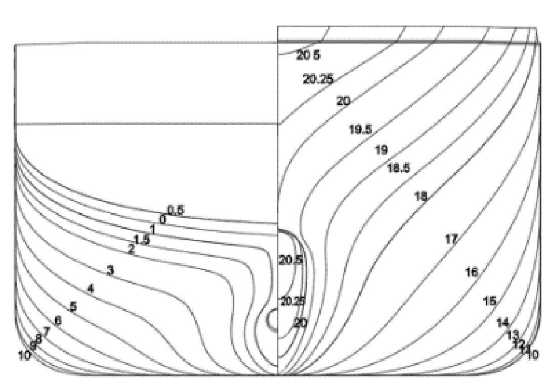
In this paper, a 13500TEU container ship is selected as the research object. The scale ratio of the model ship is 1:55. The body plan of the container ship is shown in Figure 1. The principal dimensions of the real ship and model ship are shown in

Table 1. Principal dimensions of the container ship.

Features	Real Ship	Model Ship
Length Over All (m)	366.0	6.655
Breath molded (m)	48.2	0.876
Depth molded(m)	30.2	0.549
Design draft (m)	13.5	0.245
Volume of displacement (m3)	151,016.5	2745.755

.

The features of the 13500TEU container ship at different drafts can be obtained from the ship’s loading manual. The features of the model ship can be obtained according to the scale ratio, as shown in

Table 2. Model ship features at different drafts.

Tm (m)	$\nabla$ (m3)	S (m2)	Lwl (m)	Cb	Cp	Cm	Cw	Lcb (m)	Lcf (m)
0.136	0.444	4.750	6.289	0.584	0.608	0.960	0.690	3.272	3.273
0.155	0.515	5.034	6.281	0.597	0.620	0.964	0.712	3.271	3.251
0.173	0.588	5.324	6.282	0.611	0.631	0.968	0.734	3.267	3.221
0.191	0.664	5.624	6.290	0.623	0.642	0.971	0.756	3.259	3.183
0.209	0.741	5.935	6.306	0.636	0.653	0.974	0.780	3.249	3.136
0.227	0.822	6.261	6.348	0.649	0.665	0.976	0.806	3.235	3.079
0.245	0.905	6.610	6.308	0.661	0.676	0.978	0.832	3.218	3.010
0.260	0.973	6.888	6.438	0.671	0.686	0.979	0.857	3.202	2.961
0.275	1.044	7.156	6.473	0.682	0.696	0.980	0.879	3.184	2.921
0.291	1.125	7.422	6.475	0.693	0.707	0.981	0.897	3.164	2.902

. The dimensionless features of the model ship are $T_m/B$, $L_{wl}/{\nabla }^{1/3}$, C_b, C_p, C_m, C_w, $L_{cb}/L_{wl}$, $L_{cf}/L_{wl}$, shown in

Table 3. Model ship dimensionless features at different drafts.

Tm/B	${\mathit{L}}_{\mathit{w}\mathit{l}}/{\nabla }^{1/3}$	Cb	Cp	Cm	Cw	${\mathit{L}}_{\mathit{c}\mathit{b}}/{\mathit{L}}_{\mathit{w}\mathit{l}}$	${\mathit{L}}_{\mathit{c}\mathit{f}}/{\mathit{L}}_{\mathit{w}\mathit{l}}$
0.155	8.244	0.584	0.608	0.96	0.69	0.520	0.520
0.177	7.836	0.597	0.62	0.964	0.712	0.521	0.518
0.197	7.498	0.611	0.631	0.968	0.734	0.520	0.513
0.218	7.210	0.623	0.642	0.971	0.756	0.518	0.506
0.239	6.969	0.636	0.653	0.974	0.78	0.515	0.497
0.259	6.777	0.649	0.665	0.976	0.806	0.510	0.485
0.280	6.521	0.661	0.676	0.978	0.832	0.510	0.477
0.297	6.497	0.671	0.686	0.979	0.857	0.497	0.460
0.314	6.381	0.682	0.696	0.98	0.879	0.492	0.451
0.332	6.226	0.693	0.707	0.981	0.897	0.489	0.448

.

2.2. Ship Model Resistance

The resistance test of the model ship has been conducted at the towing tank laboratory of Huazhong University of Science and Technology (HUST), China. The model ship is shown in Figure 2. The principle and detailed process of the model ship towing test is explained in the paper by Sun et al., 2016 [6]. The resistance of the model ship at different velocities and drafts are shown in

Table 4. Model ship resistance at different speeds and drafts.

Tm (m)	Rt (kgf)
	1.040 m/s	1.11 m/s	1.179 m/s	1.249 m/s	1.387 m/s	1.457 m/s	1.526 m/s
0.136	0.952	1.097	1.276	1.429	1.742	1.933	2.102
0.155	1.075	1.272	1.459	1.611	1.964	2.155	2.360
0.173	1.177	1.359	1.552	1.745	2.103	2.288	2.499
0.191	1.269	1.433	1.604	1.805	2.211	2.398	2.584
0.209	1.341	1.530	1.713	1.895	2.258	2.485	2.723
0.227	1.393	1.560	1.756	1.935	2.311	2.535	2.769
0.245	1.435	1.629	1.827	2.033	2.434	2.641	2.915
0.260	1.456	1.638	1.835	2.063	2.478	2.67	2.959
0.275	1.497	1.682	1.918	2.154	2.637	2.894	3.197
0.291	1.562	1.771	1.982	2.195	2.727	3.055	3.385

. The model ship resistance curves with velocities at different drafts are shown in Figure 3.

The model ship resistance R_t is replaced by the resistance coefficient C_t and the model ship velocity is replaced by the Froude number Fn in the process of dimensionless. The definition formulas of these two features, C_t and Fn, are shown as follows.

$$C_t=\frac{R_t}{\frac{1}{2}\times \rho \times V_m{}^2\times S}$$

(1)

$$Fn=\frac{V_m}{\sqrt{g{L}_{wl}}}$$

(2)

where, $\rho$ represents the density of water, the value of $\rho$ is 1000 kg/m³ in this paper. $g$ is the acceleration of gravity.

The resistance coefficient C_t of the model ship at different Froude numbers Fn and draft/breath T_m/B are shown in

Table 5. Model ship resistance coefficient at different Fn and T_m/B.

Tm/B	1.040 m/s		1.110 m/s		1.179 m/s		1.249 m/s		1.387 m/s		1.457 m/s		1.526 m/s
	Fn	Ct	Fn	Ct	Fn	Ct	Fn	Ct	Fn	Ct	Fn	Ct	Fn	Ct
0.155	0.132	0.371	0.141	0.375	0.150	0.387	0.159	0.386	0.177	0.381	0.185	0.383	0.194	0.380
0.177	0.132	0.395	0.141	0.410	0.150	0.417	0.159	0.410	0.177	0.406	0.186	0.403	0.194	0.403
0.197	0.132	0.409	0.141	0.414	0.150	0.419	0.159	0.420	0.177	0.411	0.186	0.405	0.194	0.403
0.218	0.132	0.417	0.141	0.414	0.150	0.410	0.159	0.411	0.177	0.409	0.185	0.402	0.194	0.395
0.239	0.132	0.418	0.141	0.418	0.150	0.415	0.159	0.409	0.176	0.396	0.185	0.394	0.194	0.394
0.259	0.132	0.411	0.141	0.404	0.149	0.404	0.158	0.396	0.176	0.384	0.185	0.381	0.193	0.380
0.280	0.132	0.401	0.141	0.400	0.150	0.398	0.159	0.394	0.176	0.383	0.185	0.376	0.194	0.379
0.297	0.131	0.391	0.140	0.386	0.148	0.383	0.157	0.384	0.175	0.374	0.183	0.365	0.192	0.369
0.314	0.131	0.387	0.139	0.382	0.148	0.386	0.157	0.386	0.174	0.383	0.183	0.381	0.191	0.384
0.332	0.130	0.389	0.139	0.387	0.148	0.384	0.157	0.379	0.174	0.382	0.183	0.388	0.191	0.392

.

3. Machine Learning Algorithms for Resistance Prediction

3.1. RBFNN

RBFNN can be used to solve the problem of the multi-dimensional fitting. The basis function, as the hidden layers of RBFNN, is a set of functions. The basis function performs nonlinear mapping on the input vector, and the output value is obtained by superimposing the linear mapping value.

In this paper, the Gaussian function [17] is selected as the basis function. The standard Gauss function can be expressed by the following formula.

$$\varphi (r)=\exp (-\frac{r^2}{2{\sigma }^2})$$

(3)

where, $r=‖X-c‖$ represents the Euclidean distance between the input vector $X$ and the center of the basis function $c$. $\sigma$ is standard deviation in Gaussian function, and it reflects the decay rate of the basis function value various with the distance from the center point. Set $c=0$, the change of Gaussian function curve with standard deviation $\sigma$ is shown in Figure 4.

The performance of RBFNN is affected by the number of center points, the position of center points and the width of basis function which, in this paper, is the standard deviation of Gaussian function $\sigma$. In this paper, the evolution strategy is used to determine the number of center points and the standard deviation, and the K-mean clustering algorithm [18] is used to determine the location of the center points.

RBFNN has been widely used in the field of ships, such as ship profile description [19] and ship seakeeping forecast [20]. The prediction of RBFNN is the cumulative result of the basis functions of different positions. The selection of the basis function affects the result of RBFNN. The Gaussian basis function can simulate multiple functions well by changing the parameters. The change of ship resistance with a single parameter, such as speed, can also be well expressed by polynomials. This is why RBFNN was chosen as the key research algorithm.

3.2. Related Machine Learning Algorithms

The BPNN [21] is one of the most widely used artificial neural network models. A typical BPNN comprises three layers: an input layer, a hidden layer, and an output layer. A different number of hidden layer nodes will affect the prediction accuracy of the BPNN. Usually, the empirical formula is used to determine the number of hidden layer neurons. The expression of the empirical formula is as follows.

$$n_2\hspace{0.33em}=\hspace{0.33em}\sqrt{n_1+n_3}\hspace{0.33em}+\hspace{0.33em}a$$

(4)

where, $n_1$, $n_2$ represents the number of the input layer and output layer nodes, respectively; a is an integer between 1 and 100. The empirical formula gives the minimum number of hidden layer nodes, $\sqrt{n_1+n_3}\hspace{0.33em}+\hspace{0.33em}1$. In this paper, in order to reduce the influence of the number of hidden layer nodes on the prediction accuracy, three BPNN models with the hidden layer nodes’ numbers of 4, 8, and 12 are used to predict resistance.

SVMs are theoretically well-justified machine learning techniques [22] with their root in structural risk minimization [23], which have also been successfully applied to many real-world domains. SVM realizes nonlinear mapping from low-dimensional space to high-dimensional space through kernel function. The most widely used kernel functions are polynomial kernel functions, radial basis functions, etc. The radial basis kernel function is adopted in this study.

RF [24] and XGBoost are ensemble learning algorithms based on decision tree. Traditional decision trees divide data according to the contribution of attributes. The best feature of the current node is used as the partition attribute. The classification/regression analysis is realized through the continuous division of data. However, the prediction results of a single decision tree usually fail to reach the expected accuracy. The accuracy of prediction can be improved by the algorithm, which contains multiple decision trees

RF randomly divides attributes and sample data into several subsets. Each subset is trained by decision tree. The performance of RF is obtained by analyzing the results of all subsets.

XGBoost contains multiple decision trees, and the next decision tree is used to make up for the fitting error of the previous decision tree. The prediction result of the XGBoost model can be expressed by the following formula.

$${\widehat{y}}_i\hspace{0.33em}=\hspace{0.33em}{\displaystyle \sum _{k=1}^K{f}_k(x_i)}$$

(5)

where, ${\widehat{y}}_i$ is the predicted value of XGBoost. K is the number of decision trees. $f_k$ represents the kth decision tree.

BPNN has been used in ship research [25]. BPNN has a strong nonlinear fitting ability. It has been proved in theory that a three-layer BPNN can approximate nonlinear functions of arbitrary precision [26,27]. Several studies [28,29] have shown that the BPNN has an advantage in the prediction task over linear regression and SVR. The SVR algorithm used in this paper has the same kernel function, the Guassian function, with the RBFNN. At the same time, the principles of the two algorithms are different. RF and XGBoost are relatively novel algorithms and have outstanding performance in machine learning competitions. This paper studies the performance of these four algorithms in ship resistance prediction as a comparison.

4. Training Process

4.1. Data Set Division

In this study, the sample ratio of the training set, the validation set, and the test set is 3:1:1. The data is randomly divided according to different drafts of the model ship for the study purpose. The resistance prediction of the model ship at different drafts is divided into two types: interpolation prediction and extrapolation prediction. The test set draft of the interpolation prediction is within the training set draft range, and the test set draft of the extrapolation prediction is outside the training set draft range. In the interpolation prediction, the model ship data at draft = 0.209 m and draft = 0.275 m are taken as the test set. The distribution of the test set is shown in Figure 5.

In the extrapolation prediction, the model ship data at draft = 0.136 m and draft = 0.291 m are taken as the test set. The distribution of the test set is shown in Figure 6.

The remaining sample data outside the test set is distributed into four subsets using the stratified sampling method in the process of searching for the optimal prediction model. Each group of subsets is considered as the validation set once, and at that time, the other three subsets are regarded as the training set. The ratio of the training set samples to the validation set samples is 3:1.

4.2. Ship Features and Predicted Values

In this research, there are three schemes of ship features and predicted value, as shown in

Table 6. Ship features and predicted value schemes.

Scheme No.	Features	Predicted Value	Prediction Model
1	Tm,$\nabla$, S, Lwl, Cb, Cp, Cm, Cw, Lcb, Lcf, Vm	Rt	BPNN, RBFNN, SVM, RF, XGBoost
2	$T_m/B$, $L_{wl}/{\nabla }^{1/3}$, Fn, Cb, Cp, Cm, Cw,$L_{cb}/L_{wl}$, $L_{cf}/L_{wl}$	Ct	RBFNN, BPNN, SVM, RF, XGBoost
3	$T_m/B$, $L_{wl}/{\nabla }^{1/3}$, Fn, Cb, Cp, Cw	Ct	RBFNN

.

The ship features in scheme 1 are all the features given in the ship’s loading manual. These features include the model ship’s main dimensional features, T_m, $\nabla$, S, L_wl; model ship form factors, C_b, C_p, C_m, C_w; and shape features, L_cb, L_cf. The width of the model ship does not change with the drafts, so it is not regarded as the ship feature. Prediction models, BPNN, RBFNN, SVM, RF, and XGBoost use these features to predict the resistance R_t of the model ship, which is the first part and an important part of this research.

In scheme 2, the model ship features and resistance R_t are dimensionless processed. The model ship resistance coefficient C_t is predicted by prediction models, BPNN, RBFNN, SVM, RF, and XGBoost using these dimensionless features.

The features in scheme 3 are parts of the ship features. Among the three model ship form features, C_b, C_p, C_m, only two of them are independent variables. So, C_b and C_p are selected as ship features for prediction. The shape features, $L_{cb}/L_{wl}$ and $L_{cf}/L_{wl}$, are abandoned in scheme 3. The RBFNN is also used to predict the model ship’s resistance coefficient. For the convenience of expression, the three feature schemes are marked as F1, F2, F3 in the following text, respectively.

4.3. Model Parameters Selection

To ensure the best performance of each machine learning prediction models, the parameters of the prediction model need to be tuned manually or automatically. In this paper, the evolutionary strategies are used to find the optimal parameters of each machine learning model. In the process of parameter tuning, initially, a certain number of parameter sets are randomly generated within the search range as the parent set. The subset is generated through the cross mutation of the parent set. Calculate the fitness of the parent set and the subset, and select part of parameter sets with better fitness to be the parent set of the next generation. The evolution is stopped until the number of the iteration meets the requirements, and the subset with the best fitness is selected as the final parameters of the prediction model. The parameters properties and the searching range of the five models are shown in

Table 7. The parameter properties of the prediction model and searching ranges.

Models	Parameters	Description	Default Value	Searching Range
RBFNN	k	Number of center points	‘auto’	(1, 42)
	$\delta$	variance	1	(1, 300)
BPNN	h	Number of hidden layer nodes	None	4, 8, 12
SVR	C	Regularization parameter.	1	(1, 100)
	gamma	Kernel coefficient for the ‘rbf’, ‘poly’ and ‘sigmoid’. If gamma is ‘auto’, then 1/n features will be used instead.	‘auto’	(0, 1)
RF	n-estimators	The number of trees in the forest.	10	(10, 300)
	max depth	The maximum depth of the tree. If None, then the nodes are expanded until all leaves are pure or until all leaves contain less than min samples split samples.	None	(1, 30)
	min samples split	The minimum number of samples required to split an internal node.	2	(1, 30)
	min samples leaf	The minimum number of samples required to be at a leaf node.	1	(1, 30)
XGBoost	n-estimators	The number of trees in the forest.	100	(10, 300)
	min child weight	The minimum sum of the instance weights(Hessian) needed in a child.	1	(1, 30)
	max depth	The maximum depth of the tree.	3	(1, 30)

.

In order to reduce the influence of the evolution strategies parameters on the selection of model parameters, the mutation strength boundary of all the model parameters is set to 2/3 of the searching range, and the number of iterations is set to 200.

4.4. Evaluation Metric of Prediction Models

In this paper, the Maximum of Relative Absolute Error (MRAE) is used to evaluate the accuracy of prediction models. The formula of Relative Absolute Error (RAE) and MRAE are shown as follows.

$$RAE=\left|\frac{Valu{e}_E-Valu{e}_P}{Valu{e}_E}\right|\hspace{0.33em}\times \hspace{0.33em}100\%$$

(6)

$$MRAE\hspace{0.33em}=\hspace{0.33em}\hspace{0.33em}\max \hspace{0.33em}\left\{RA{E}_1,RA{E}_2,\cdot \cdot \cdot ,RA{E}_n\right\}$$

(7)

where, Value_E is the experimental value, Value_P is the predicted value, RAE_i represents the RAE of the ith sample.

In the training process, the model parameters that minimize the MRAE of the training set and the validation set are taken as the optimal parameters of the prediction model. The prediction model with the optimal parameters is used to predict the resistance of the test set. The complete training process is shown in Figure 7.

5. Predicted Results and Comparison

5.1. Comparison of the Predicted Results

The number of hidden layers will affect the performance of the BPNN. This paper studies the prediction results of BPNN with three different hidden layer numbers of 4, 8, and 12. The interpolation and extrapolation prediction results of the model ship resistance R_t and model ship resistance coefficient C_t using BPNN are shown in

Table 8. The prediction results of model ship resistance R_t using backpropagation neural network BPNN.

Interpolation Method	Number of Hidden Layers	Rt (kgf)
		1.040 m/s	1.11 m/s	1.179 m/s
Interpolation	4	2.588	3.341	3.771
	8	2.773	3.432	3.885
	12	3.123	3.841	3.725
Average value		2.828	3.538	3.794
Extrapolation	4	2.583	2.922	9.986
	8	2.204	2.828	9.990
	12	2.331	3.147	10.464
Average value		2.372	2.966	10.147

and

Table 9. The prediction results of model resistance coefficient C_t using backpropagation neural network BPNN.

Interpolation Method	Number of Hidden Layers	MRAE (%)
		Training Set	Validation Set	Test Set
Interpolation	4	6.369	5.187	3.260
	8	6.398	5.202	3.264
	12	6.270	5.091	3.287
Average value		6.346	5.160	3.270
Extrapolation	4	5.236	4.109	13.247
	8	5.234	4.118	13.254
	12	5.178	4.100	13.081
Average value		5.216	4.109	13.194

, respectively. It is not difficult to find that the prediction results of these three BPNN models are not much different. The average value of the three BPNN models prediction results is taken as the performance of the BPNN and compare it with other prediction models. The MRAE of the training set, the validation set, and the test set of different ship resistance prediction models are shown in

Table 10. The prediction results of different models.

Prediction Type	Feature Schemes	Prediction Model	MRAE (%)
			Training Set	Validation Set	Test Set
Interpolation	F1	RBNN	2.828	3.538	3.794
		RBFNN	1.244	2.006	2.006
		SVM	6.988	6.471	6.866
		RF	17.453	17.619	9.957
		XGBoost	3.471	3.463	6.712
	F2	RBNN	6.346	5.160	3.270
		RBFNN	1.094	1.733	1.731
		SVM	7.350	6.410	6.072
		RF	3.633	4.161	2.546
		XGBoost	0.959	2.44725	3.3955
	F3	RBFNN	1.228	1.827	1.981
Extrapolation	F1	RBNN	2.372	2.966	10.147
		RBFNN	1.386	1.397	7.718
		SVM	6.514	6.187	14.799
		RF	14.097	11.952	32.125
		XGBoost	1.755	3.647	16.398
	F2	RBNN	5.216	4.109	13.194
		RBFNN	1.472	1.724	10.431
		SVM	7.350	6.730	6.061
		RF	3.906	4.092	10.841
		XGBoost	0.491	2.251	10.169
	F3	RBFNN	1.481	1.636	23.626

.

In F1, the sample data is the actual model ship features and model ship resistance. In F2, the sample data was processed in a dimensionless manner. The sample data in F3 is partially dimensionless features. The interpolation and extrapolation prediction results comparison of different prediction models are shown in Figure 8 and Figure 9. The following conclusions can be drawn from the prediction results.

•  The extrapolation prediction accuracy of the model ship resistance is much lower than that of the interpolation prediction.
•  For the interpolation prediction, the dimensionless processing of data can improve the resistance prediction accuracy of all models.
•  Among all the interpolation schemes, using dimensionless ship features to estimate ship resistance coefficient C_t based on RBFNN has the highest accuracy. The MRAE of the RBFNN prediction model is 1.731%. All interpolation prediction schemes using RBFNN have good performance. The results show that RBFNN is suitable for predicting the model ship resistance with an interpolated draft. The accuracy of using the RF model to predict ship resistance coefficient is also good, and its MRAE is 2.546%. They were followed by other prediction models.

The optimal predicted resistance coefficient C_t is converted to the corresponding resistance R_t. The experimental values and predicted values of each sample point in the test set are shown in

Table 11. The experimental values and predicted values of test set by the best performing model.

Tm (m)	Vm (m/s)	Fn	Experimental Value		Predicted Value		RAE (%)
			Ct × 103	Rt (kgf)	Ct × 103	Rt (kgf)
0.209	1.040	0.132	4.099	1.341	4.063	1.329	0.875
	1.110	0.141	4.105	1.530	4.056	1.510	1.196
	1.179	0.150	4.074	1.713	4.029	1.690	1.095
	1.249	0.159	4.016	1.895	3.988	1.876	0.691
	1.387	0.176	3.880	2.258	3.889	2.255	0.220
	1.457	0.185	3.870	2.485	3.842	2.461	0.729
	1.526	0.194	3.866	2.723	3.805	2.679	1.561
0.275	1.040	0.131	3.795	1.497	3.840	1.509	1.195
	1.110	0.139	3.743	1.682	3.808	1.708	1.728
	1.179	0.148	3.783	1.918	3.771	1.911	0.316
	1.249	0.157	3.786	2.154	3.736	2.126	1.321
	1.387	0.174	3.758	2.637	3.693	2.593	1.731
	1.457	0.183	3.738	2.894	3.697	2.863	1.084
	1.526	0.192	3.764	3.197	3.726	3.163	1.019

. The curves of C_t versus Fn and the curves of R_t versus V_m at draft = 0.209 m and draft = 0.275 m are shown in Figure 10 and Figure 11, respectively.

• Among all the extrapolation schemes, using dimensionless ship features to estimate ship resistance coefficient C_t based on SVM has the highest accuracy. The MRAE of the model prediction is 6.072%. The MRAE of the training set, validation set, and test set of this model is not much different, all greater than 6%. The performance of the RBFNN model that uses ship features to predict resistance R_t in the test set is slightly inferior to the SVM model with the MRAE of 7.718%, and better than other prediction models.

For the extrapolation prediction, the resistance coefficient C_t obtained by the SVM prediction model is converted to the corresponding ship resistance R_t. The performances of the SVM model and the RBFNN model are shown in Figure 12 and Figure 13.

In the actual situation, it is not initially known that the predicted draft belongs to a particular type of extrapolation or interpolation. Combining the resistance prediction results under the draft states of interpolation and extrapolation, the RBFNN prediction model based on F1 is undoubtedly the best one among all the models mentioned in this article.

5.2. Comparison of the RBFNN and the Modified Admiralty Coefficient

The accurate prediction of ship power/resistance has always been a hot issue for designers. The most commonly used method is the admiralty coefficient, which is expressed as: ships with similar hull form, scale and speed have the same admiralty coefficient. The relationship between ship resistance, effective power and the admiralty coefficient is shown in the following formula.

$$P_e=Rv\hspace{0.33em}=\hspace{0.33em}\frac{{\Delta }^{2/3}{v}^3}{C}$$

(8)

where, P_e is the effective power. R is the ship resistance. v is the ship velocity. Δ is the displacement. C is the admiralty coefficient.

The admiralty coefficient method, although a useful and simple estimation method, is a somewhat ‘blunt instrument’ when used in power estimation since it fails to effectively distinguish between the power and hull-related parameters. The effectiveness of the admiralty coefficient formula should be evaluated in the engineering.

Many researchers [30,31,32] have undertaken a significant amount of work on the estimation method of the power curve. In the paper by Tu in 2018, the fixed power exponent of admiralty coefficient is replaced by $2/3\times (C_b+C_w^{})$, and the power curves of the container ship is estimated by the modified admiralty formula.

$$\frac{P_{s2}}{P_{s1}}={\left(\frac{{\Delta }_2}{{\Delta }_1}\right)}^{1-\frac{2\times (C_b+C_w)}{3}}$$

(9)

The power of the model ship at 0.191 m draft is taken as P_s1; the power of the model ship at 0.209 m draft P_s2 can be estimated by the modified formula. The parameters C_b and C_w belong to the model ship at 0.191 m draft. Similarly, using the data of 0.260 m draft, the power of the model ship at 0.275 m draft can be obtained. At the draft = 0.209 m and draft = 0.275 m, the ship power is estimated by the modified admiralty formula, and the resistance of the model ship is estimated by RBFNN prediction model. The absolute value of the MRAE comparison of the two methods is shown in

Table 12. The comparison of the MRAE obtained by the two estimate methods.

Ship Type	Model Draft (m)	Modified Admiralty Formula (%)	RBFNN Resistance Prediction (%)
13500TEU	0.209	3.18	1.561
	0.275	6.46	1.731

.

Compared with the previous modified admiralty formula, the prediction accuracy of the RBFNN prediction model has been greatly improved.

6. Conclusions and Discussion

This paper uses five machine learning methods—BPNN, RBFNN, SVM, RF, and XGBoost—to predict the model ship resistance of a 13500TEU container ship at different drafts using actual ship data and dimensionless ship data. There are two states of interpolation and extrapolation for the resistance prediction. The optimal parameters of each model are obtained through evolutionary strategies. Compared with other prediction models, the following conclusions can be drawn:

•  The model ship resistance can be predicted more accurately by RBFNN for the interpolation prediction. The prediction accuracy of the RBFNN has been further improved using by dimensionless ship features and the total resistance coefficient. Good prediction results can be obtained by using a part of dimensionless features.
•  For the extrapolation prediction, the prediction results of R_t using RBFNN have a high accuracy (7.718%), which is second only to the prediction accuracy (6.072%) of C_t using SVM. The performance of C_t prediction using dimensionless features is poor.
•  For the resistance prediction of container ships, the RBFNN using actual ship characteristics is a better choice.
•  Compared with the modified admiralty coefficient, the prediction accuracy of the RBFNN method is significantly improved, and has more value in terms of engineering applications.

For a prediction problem, there is a suitable prediction method. Reasonable data processing methods can improve prediction accuracy. If there are a lot of data for different container ships, the prediction ideas mentioned in the paper can be used to build a ship resistance prediction model to predict the resistance of other container ships.

References

- Jeong, S.Y.; Choi, K.; Kang, K.J.; Ha, J.S. Prediction of ship resistance in level ice based on empirical approach. Int. J. Nav. Arch. Ocean Eng. 2017, 9, 613–623. [Google Scholar] [CrossRef]
- Liu, G.; Guo, C.; Li, M.; Huang, C. Analysis and Comparison of Model Trial Results and Ship Resistance Atlas Calculation. Chin. J. Ship Res. 2014, 9, 38–42. [Google Scholar]
- Tu, H.; Yang, Y.; Zhang, L.; Lyu, X.; Song, L.; Guan, Y.M.; Sun, J. A modified admiralty coefficient for estimating power curves in EEDI calculations. Ocean Eng. 2018, 150, 309–317. [Google Scholar] [CrossRef]
- Guo, B.J.; Deng, G.B.; Steen, S. Verification and validation of numerical calculation of ship resistance and flow field of a large tanker. Ships Offshore Struct. 2013, 8, 3–14. [Google Scholar] [CrossRef]
- Li, S.Z.; Zhao, F.; Ni, Q.-J. Bow and stern shape integrated optimization for a full ship by a simulation-based design technique. J. Ship Res. 2014, 58, 83–96. [Google Scholar] [CrossRef]
- Sun, J.; Tu, H.; Chen, Y.; Xie, D.; Zhou, J. A Study on Trim Optimization for a Container Ship Based on Effects due to Resistance. J. Ship Res. 2016, 60, 30–47. [Google Scholar] [CrossRef]
- Lv, X.; Wu, X.; Sun, J.; Tu, H. Trim Optimization of Ship by a Potential-Based Panel Method. Adv. Mech. Eng. 2013, 12, 378140. [Google Scholar] [CrossRef] [Green Version]
- Lyu, X.; Tu, H.; Xie, D.; Sun, J. On Resistance Reduction of Hull by Trim Optimization. Brodogradnja. 2018, 69, 1–13. [Google Scholar] [CrossRef] [Green Version]
- Atmane, K.; Ma, H.; Qing, F. Convolutional Neural Network Based on Extreme Learning Machine for Maritime Ships Recognition in Infrared Images. Sensors 2018, 18, 1490. [Google Scholar]
- Niu, H.; Emma, O.; Peter, G. Ship localization in Santa Barbara Channel using machine learning classifiers. J. Acoust. Soc. Am. 2017, 142, 455–460. [Google Scholar] [CrossRef]
- Guan, B.; Yang, W.; Wang, Z.; Tang, Y. Ship roll motion prediction based on ℓ1 regularized extreme learning machine. PLoS ONE 2018, 13, e0206476. [Google Scholar] [CrossRef] [Green Version]
- Gkerekos, C.; Lazakis, I.; Theotokatos, G. Machine learning models for predicting ship main engine Fuel Oil Consumption: A comparative study. Ocean Eng. 2019, 188, 1–14. [Google Scholar] [CrossRef]
- Ling, J.; Kurzawski, A.; Templeton, J. Reynold averaged turbulence modelling using deep neural network with embedded invariance. J. Fluid Mech. 2016, 807, 155–166. [Google Scholar] [CrossRef]
- Wang, J.; Wu, J.; Xiao, H. Physics-informed machine learning approach for reconstructing Reynolds stress modeling discrepancies based on DNS data. Phys. Rev. Fluids. 2017, 2, 034603. [Google Scholar] [CrossRef] [Green Version]
- Rabault, J.; Kuchta, M.; Jensen, A.; Réglade, U.; Cerardi, N. Artificial neural networks trained through deep reinforcement learning discover control strategies for active flow control. J. Fluid Mech. 2019, 856, 281–302. [Google Scholar] [CrossRef] [Green Version]
- Raissi, M.; Wang, Z.; Triantafyllou, M.S.; Karniadakis, G.E. Deep learning of vortex-induced vibrations. J. Fluid Mech. 2019, 861, 119–137. [Google Scholar] [CrossRef] [Green Version]
- Bugmann, G. Normalized Gaussian radial basis function networks. Neurocomputing 1998, 20, 97–110. [Google Scholar] [CrossRef]
- Grabusts, P.S. A Study of Clustering Algorithm Application in RBF Neural Networks. In Scientific Proceedings of Riga Technical University; RTU: Riga, Latvia, 2001; pp. 50–57. [Google Scholar]
- Ban, D.; Ljubenkov, B. Global Ship Hull Description using Single RBF. In Proceedings of the IMAM 2015—16th International Congress of the International Maritime Association of the Mediterranean, Pula, Croatia, 21–24 September 2015. [Google Scholar]
- Yin, J.C.; Wang, N.N. Online grey prediction of ship roll motion using variable RBFN. Appl. Artif. Intell. 2013, 27, 941–960. [Google Scholar] [CrossRef]
- Rumelhart, D.E.; Hinton, G.E.; Williams, R.J. Learning representations by back-propagating errors. Nature 1986, 323, 533–536. [Google Scholar] [CrossRef]
- Shawe-Taylor, J.; Sun, S. A review of optimization methodologies in support vector machines. Neurocomputing 2011, 74, 3609–3618. [Google Scholar] [CrossRef]
- Shawe-Taylor, J.; Bartlett, P.; Williamson, R.; Anthony, M. Structural risk minimization over data-dependent hieraichies. IEEE Trans. Inf. Theory. 1998, 44, 1926–1940. [Google Scholar] [CrossRef] [Green Version]
- Breiman, L. Random forests. Mach. Learn. 2001, 45, 5–23. [Google Scholar] [CrossRef] [Green Version]
- Zhou, H.; Chen, Y.; Zhang, S. Ship Trajectory Prediction Based on BP Neural Network. J. Artif. Intell. 2019, 1, 29. [Google Scholar] [CrossRef]
- Hornik, K.; Stinchcombe, M.; White, H. Multilayer feedforward networks are universal approximators. Neural Netw. 1989, 2, 359–366. [Google Scholar] [CrossRef]
- Xu, B.; Zhang, H.; Wang, Z.; Wang, H.; Zhang, Y. Model and Algorithm of BP Neural Network Based on Expanded Multichain Quantum Optimization. Math. Probl. Eng. 2015, 2015, 1–11. [Google Scholar] [CrossRef] [Green Version]
- Lee, S.; Choeh, J.Y. Predicting the helpfulness of online reviews using multilayer perceptron neural networks. Expert Syst. Appl. 2014, 41, 3041–3046. [Google Scholar] [CrossRef]
- Wong, T.C.; Chan, H.K.; Lacka, E. An ANN-based approach of interpreting user-generated comments from social media. Appl. Soft. Comput. 2017, 52, 1169–1180. [Google Scholar] [CrossRef] [Green Version]
- Tu, H.; Yang, Y.; Lyu, X.; Xie, D.; Gao, X.; Sun, J. An inverse design method for body surface of given target pressure distribution. Ocean Eng. 2018, 163, 737–747. [Google Scholar] [CrossRef]
- Duan, B.; Deng, K.; Song, W.; Yuan, H.-L. Calculation and optimization of energy efficiency design index for large container ship. Nav. Architect. Ocean Eng. 2012, 3, 22–30. [Google Scholar]
- Yuan, Y.-S. Vessel Velocity Prediction toward Model Demonstration and System Realization. Master’s Thesis, Dalian University of Technology, Dalian, China, 2009. [Google Scholar]
Figure 1.
Body plan of the 13500 transmission extension unit (13500TEU) container ship.
Figure 2.
The test model of the 13500TEU container ship.
Figure 3.
The model ship resistance changes with velocities at different drafts.
Figure 4.
The change of Gaussian function curve with standard deviation.
Figure 5.
The distribution of test set samples for interpolation prediction.
Figure 6.
The distribution of test set samples for extrapolation prediction.
Figure 7.
The training process of prediction models.
Figure 8.
The Maximum of Relative Absolute Error (MRAE) of interpolation prediction under different models.
Figure 9.
The MRAE of extrapolation prediction under different models.
Figure 10.
The curves of Ct versus Fn at the drafts of 0.209 m and 0.275 m by the best performing model.
Figure 11.
The curves of Rt versus Vm at the drafts of 0.209 m and 0.275 m by the best performing model.
Figure 12.
The ship resistance prediction results of the SVM and RBFNN models at the draft = 0.136 m.
Figure 13.
The ship resistance prediction results of the SVM and RBFNN models at the draft = 0.209 m.