Article

A Barotropic Solver for High-Resolution Ocean General Circulation Models

1
First Institute of Oceanography, and Key Laboratory of Marine Science and Numerical Modeling, Ministry of Natural Resources, Qingdao 266061, China
2
Laboratory for Regional Oceanography and Numerical Modeling, Pilot National Laboratory for Marine Science and Technology, Qingdao 266237, China
3
Shandong Key Laboratory of Marine Science and Numerical Modeling, Qingdao 266061, China
4
Vacation BU, Trip.com Group Limited, Shanghai 200335, China
5
School of Software, Shandong University, Jinan 250101, China
*
Author to whom correspondence should be addressed.
J. Mar. Sci. Eng. 2021, 9(4), 421; https://doi.org/10.3390/jmse9040421
Submission received: 8 March 2021 / Revised: 8 April 2021 / Accepted: 9 April 2021 / Published: 14 April 2021
(This article belongs to the Special Issue Ocean Modelling in Support of Operational Ocean and Coastal Services)

Abstract

:
High-resolution global ocean general circulation models (OGCMs) play a key role in accurate ocean forecasting. However, the models of the operational forecasting systems are still not in high resolution due to the subsequent high demand for large computation, as well as the low parallel efficiency barrier. Good scalability is an important index of parallel efficiency and is still a challenge for OGCMs. We found that the communication cost in a barotropic solver, namely, the preconditioned conjugate gradient (PCG) method, is the key bottleneck for scalability due to the high frequency of the global reductions. In this work, we developed a new algorithm—a communication-avoiding Krylov subspace method with a PCG (CA-PCG)—to improve scalability and then applied it to the Nucleus for European Modelling of the Ocean (NEMO) as an example. For PCG, inner product operations with global communication were needed in every iteration, while for CA-PCG, inner product operations were only needed every eight iterations. Therefore, the global communication cost decreased from more than 94.5% of the total execution time with PCG to less than 63.4% with CA-PCG. As a result, the execution time of the barotropic modes decreased from more than 17,000 s with PCG to less than 6000 s with CA-PCG, and the total execution time decreased from more than 18,000 s with PCG to less than 6200 s with CA-PCG. Besides, the ratio of the speedup can also be increased from 3.7 to 4.6. In summary, the high process count scalability when using CA-PCG was effectively improved from that using the PCG method, providing a highly effective solution for accurate ocean simulation.

1. Introduction

Ocean general circulation models (OGCMs) have become increasingly important for understanding oceanic dynamic processes and ocean environment forecasting. In recent years, OGCMs have been developed with finer resolution (10–100 km for eddy-resolving ocean models) and more physical procedures due to increasing scientific requirements. Accuracy is one of the important goals of ocean simulation and forecasting. In general, OGCMs with finer horizontal resolution can provide more accurate results [1]. However, the computational cost will be almost three orders of magnitude if the horizontal resolution is fined by one order of magnitude [2,3]. For an operational forecasting system, the computation should be finished within 1∼2 h. So, the parallel efficiency becomes a great challenge for OGCMs. Due to the low parallel efficiency, current global operational forecasting systems are still in 0.1° (∼10 km) to 1° (∼100 km) resolution, which falls far short of expectations. Therefore, with the resolution finer, the demand for improving computational performance is more and more urgent.
To increase the computational efficiency of OGCMs, the hydrostatic primitive equations for momentum can be solved using a split-explicit, time-stepping scheme that requires special treatment and coupling between barotropic and baroclinic modes. The baroclinic mode is used for three-dimensional prognostic variables, which are the slow processes, such as the advective term, while the barotropic mode solves the free-surface and associated barotropic velocity equations, such as surface inertial gravity wave, which are the fast processes. To improve the simulation efficiency, a finite number of barotropic time steps were carried out within each baroclinic step (details in Appendix A). In barotropic mode, the implicit free-surface method is common because it allows a large time step to efficiently calculate the fast gravity mode [4,5]. But this method requires solving elliptic equations (details are discussed in Section 2). One of the commonly used methods of solving an elliptic equation is the conjugate gradient (CG) method [6]. To reduce the execution time of the CG method, one way is to reduce the communication costs by reducing the number of iterations to convergence. Thus, preconditioning is commonly used for the CG method to reduce the number of iterations, assuming the cost of preconditioning is reasonable [7], which has been widely applied in OGCMs [8,9,10]. As the Preconditioned CG method (PCG) method used in OGCMs requires the calculation of global variables, which also expects a large number of global reductions, it becomes the bottleneck when the model is run in the large-scale parallel computation. To further reduce the associated communication cost and improve scalability, [11] tried to apply a preconditioned Classical Stiefel Iteration method instead of the PCG method in the Parallel Ocean Programme to solve the elliptic system of equations in the barotropic mode, which requires no global reduction except for checking convergence. However, the PCG method is still popular and widely used due to less requirement in memory, better stability, and faster and clearer representation. Thus, the other way to reduce the number of global reductions to improve the large-scale efficiency of the PCG method is necessary and rarely done before.
The Nucleus for European Modelling of the Ocean (NEMO) is a state-of-the-art OGCM that has been widely used by ocean and climate communities for oceanographic, forecasting, and climate studies [9]. The barotropic solver recommended in NEMO is also the PCG method because it can effectively solve elliptic equations with vector computers. When using thousands of processes, the PCG method in NEMO scales poorly (Figure 1), as do other OGCMs. After analyzing, we found that the poor scaling performance of the PCG method was caused by the operation of global reductions (i.e., function MPI_Allreduce combines values from all processes and distributes the result back to all processes), which could account for more than 96% of the total execution time when using more than 8000 processes (Figure 2).
In this study, we developed a new method, namely, a communication-avoiding Krylov subspace method with PCG (CA-PCG), to reduce the number of global reductions and improve the PCG method in the barotropic mode in NEMO. The results showed a high decrease in the total execution time for the high-resolution simulation with NEMO and provided a reference for the OGCMs using PCG solver for developing effective measures to improve the scalability on large scales.

2. Materials and Methods

2.1. NEMO Model

The Nucleus for European Modelling of the Ocean (NEMO) is a framework of ocean-related engines, namely, OPA (O’cean PArall´elis´e) for the ocean dynamics and thermodynamics, LIM2 (Louvain-la-Neuve Ice Model version 2) for the sea–ice dynamics and thermodynamics, and TOP3 (Tracer in the Ocean Paradigm version 3) for the biogeochemistry [9]. The ocean component of NEMO was developed from the OPA model, as described in [12]. This model has been used for a wide range of applications, both regional and global, as a forced ocean model and as a model coupled with the sea-ice and/or the atmosphere. The barotropic mode optimized in this study is a procedure that solves the free-surface, and associated barotropic velocity equations belong to the OPA model.

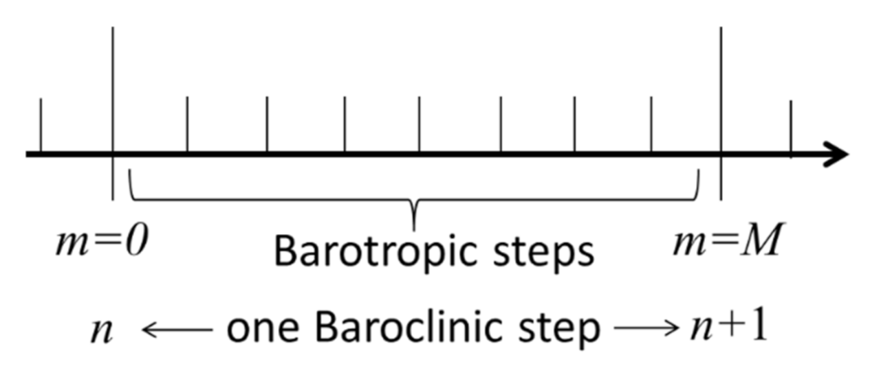
2.2. Barotropic Solver

As discussed above, the solution of an elliptic equation is the most time-consuming part of the barotropic mode for large-scale clusters. Here, the elliptic equation is shown [11]:
[ · H τ ] η n + 1 = ψ η n , η n 1 , τ
where H represents the depth of the ocean, τ is the time step, η n is the sea surface height (SSH) at the n-th time step, and ψ is the function of the influence that the previous states of the SSH and forcing have on the next state.
At each time step, the time derivative of the SSH at the next time step is solved with an elliptic equation. Equation (1) is discretized into a two-dimensional orthogonal curvilinear grid using a five-point stencil in NEMO and can be reorganized into a linear symmetric system Ax = b. The idea of the PCG method is to search for the solution of x.

2.3. NEMO PCG Solver

The PCG used in NEMO is a modified typical PCG. However, the modification does not reduce the operation of the global reductions (MPI_Allreduce). As global reductions are the main bottleneck of the NEMO model, the optimization was still based on the typical PCG for simplicity in this study. The typical PCG method (Algorithm A1) contains three major parts: computing, boundary updating, and global reduction. There are matrix-vector multiplications (MVMs) and vector–vector multiplications (VVMs) in this computation, displaying good scalability. The time cost of boundary updating is required to update the halo area after an MVM, but there is no scalability issue for large-scale clusters. The cost of global reductions required by the inner product, is the key problem in a large-core count cluster. The details of the communication costs and performance analysis are illustrated in Appendix B.

2.4. CA-PCG Solver

Optimization of NEMO scalability, which was mainly caused by the global reduction in the PCG solver, has rarely been studied until now. To solve this problem, a communication-avoiding Krylov subspace method was implemented with PCG (CA-PCG), according to Carson’s work [13]. For PCG, inner product operation is needed for each iteration, which means a global reduction cost for each iteration. However, for CA-PCG, all of the iterations are divided into two layers of loops. The global reductions are only needed in the outer loop. Since we used the same preconditioner for PCG, the iteration number K should not change. If s is the inner loop count, then the outer loop count will be K/s, which means one global reduction is needed after every s iterations. After multiple tests, the inner loop count s was set as 8 in this study. Then the frequency of inner product operation was decreased to every eight iterations. Moreover, the global communication cost could decrease dramatically, and the high-core count scalability could be improved effectively. The pseudocode for the CA-PCG algorithm designed for NEMO is shown in Appendix C.

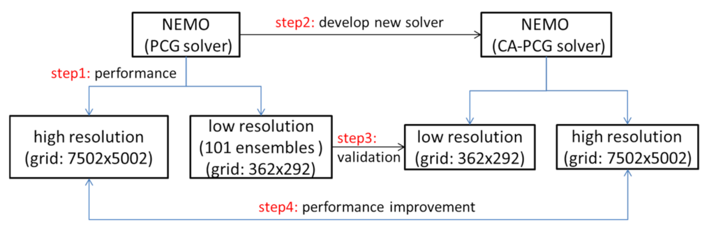
2.5. Experimental Description

The NEMO model optimized in this study was version 3.6. To assess the performance of the NEMO model and the validity of the model results after optimization using the CA-PCG method, two experiments were designed: a low-resolution experiment, named ORCA1, with a horizontal grid resolution of nearly 100 km (grid dimensions: 362 × 292) and a high-resolution experiment, named GYRE, with a horizontal grid resolution of nearly 5 km (grid dimensions: 7502 × 5002). The optimization of the NEMO model using the CA-PCG solver was mainly to reduce the communication costs. So, the performance improvement should be more effective on large-scale simulations than on a small scale. Thus, we used a small-scale experiment to validate the results’ accuracy and a large-scale experiment to test the scalability of this approach. The flow chart of the total experiments is shown in Figure 3. First, a high-resolution experiment was designed to evaluate the performance of the NEMO model with a PCG solver. Second, a new solver, i.e., CA-PCG solver, was developed and applied to the NEMO model. The next step was to validate the accuracy of the model results after optimization by comparing them with those from ensembles with PCG solver using low-resolution experiments. Last, the improvement of the performance of the NEMO model with the CA-PCG solver was tested using a high-resolution experiment. The description of the parallel platform used in this study is provided in Appendix D.

2.5.1. Low-Resolution Simulation

ORCA1 is one of the most frequently used horizontal grid resolutions in NEMO. The grid was derived from https://forge.ipsl.jussieu.fr/nemo/ (accessed on 10 April 2021), while the bathymetry file was generated by referring to http://www.noc.ac.uk/ (accessed on 10 April 2021). The initial conditions of temperature and salinity were from a combination of the World Ocean Atlas (WOA) 2009 [14,15] and the Polar Science Center Hydrographic Climatology (PHC) version 3 (updated from [16]) data. We also used the WOA 2009 and PHC v3.0 temperature data as observations to validate the model results (details in Section 2.6). The atmospheric forcing data were from the climatology Coordinated Ocean-ice Reference Experiments phase II (CORE-II) forcing data set [17,18]. The time step used in this experiment was 3600 s (i.e., the rn_rdt parameter in NEMO was set to 3600). Experiments using the PCG and CA-PCG solvers were designed, regarded as ORCA1_PCG and ORCA1_CAPCG, respectively. Besides, to validate the model results, an ensemble consisting of 101 ocean simulations using the PCG solver was also created.

2.5.2. High-Resolution Simulation

The idealized GYRE application in NEMO was presented to test and analyze the scalability of high-resolution simulation on a large scale. There was no file Input/Output other than the reading of the workload definition during initialization. This experiment used a time step of 7200 s (rn_rdt = 7200). To guarantee that the total execution time of all of the experiments was no less than 3 min, the experiments were run for 1000 steps. Corresponding experiments using the PCG and CA-PCG solvers were also designed, regarded as GYRE_PCG and GYRE_CAPCG, respectively. Notably, each experiment was repeated three times, and the mean values of the execution time were discussed.

2.6. Community Earth System Model (CESM) Port-Verification Tool

The methodology we used to validate the results was the Community Earth System Model (CESM) port-verification tool (CESM-PVT), which was developed to determine whether a change in CESM would result in distinguished biases from the natural variability of the system [19]. First, in [19], an ensemble E = {X1, X2, … Xm} consisting of 101 simulations, which differed only in a random perturbation of the initial temperature condition at the order of 10−14, was run. At a given point j, we had a series of possible results for each variable X from the ensemble E = {X1(j), X2(j), … Xm(j)}. Then, the mean and standard deviation of this series at a given point j was defined as μ j and δ j , respectively. The root mean square z-score (RMSZ) of the ensemble data was calculated as follows.
R M S Z X =   1 n j = 1 n X j μ j δ j 2
where n is the total number of grid points in X. Moreover, the RMSZ score of the new case was also calculated. If this RMSZ fell within the distribution of the ensemble’s RMSZ, then the result was considered to have passed the accuracy test. The details could refer to [11,19].
According to [19], this methodology not only benefits the model data of the CESM, but is also applicable for evaluating the data of other simulations. To verify the accuracy of the NEMO model using the CA-PCG solver, we also considered 101 simulations, which were the same as for the ORCA1_PCG experiment, except for a random perturbation of the initial ocean temperature at the order of 10−14. The ensemble runs here were 10 years in length, which is a long enough duration for an ocean model to become stable after a disturbance.
To verify the result, we did some revisions to the CESM-PVT method. First, to increase the reliability, we treated observations (WOA + PHC data) instead of the mean value of ORCA1_PCG ensemble members as the “reference value” here. This is because the only thing we cared about was whether the model results were consistent with observations, no matter before or after optimization. Second, for each ensemble member, the global mean value was calculated first, and then the mean biases and standard deviations compared to the observed global mean value were obtained at each time point. The global mean value of the CA-PCG experiment and the mean bias were calculated at the same time. Finally, the mean biases of each ensemble member and the CA-PCG experiment were divided by the corresponding standard deviations at each time point to obtain the z-score biases, respectively. We revised the CESM-PVT method by comparing the global mean value instead of the point-to-point value because the biases may be magnified at a specific point. For example, when the results between the ORCA1_PCG ensembles and observations are very close, any destabilization in the ORCA1_CAPCG results may lead to a large deviation after being divided by these extremely small standard deviations. Verification using the global mean value would avoid this issue effectively. Besides, the global mean value is an effective indicator of ocean simulation evaluation. The equation is revised as follows.
Z X =   j = 1 n X j n μ j δ j
where j = 1 n X j n is the calculation of global mean value at a given point j. The μ j represents the value in observation. The δ   bs is the standard deviation of the ensemble time series.

3. Results

3.1. Validity of the Results Using the CA-PCG Solver

We verified the model results using the CA-PCG solver with the revised CESM-PVT method shown above. Figure 4 shows the distribution of the z-score biases of the temperature variable in 101 ensemble runs with the PCG solver and the CA-PCG experimental result. As the observation of temperature is more accessible than other variables and is also one of the fundamental physical quantities in ocean simulation, we chose the three-dimensional temperature field for this evaluation. To match the accuracy of CESM-PVT, the variable’s z-score bias of the experiment using the CA-PCG solver should be no larger than those of the ensemble simulations. As shown in Figure 4, the CA-PCG experimental result’s z-score bias fell into the distribution of the ensemble z-score biases, showing good consistency with the results simulated using the PCG solver. Above all, the model results simulated using the CA-PCG solver were accurate, and the CA-PCG solver can be used in the NEMO model in future research.

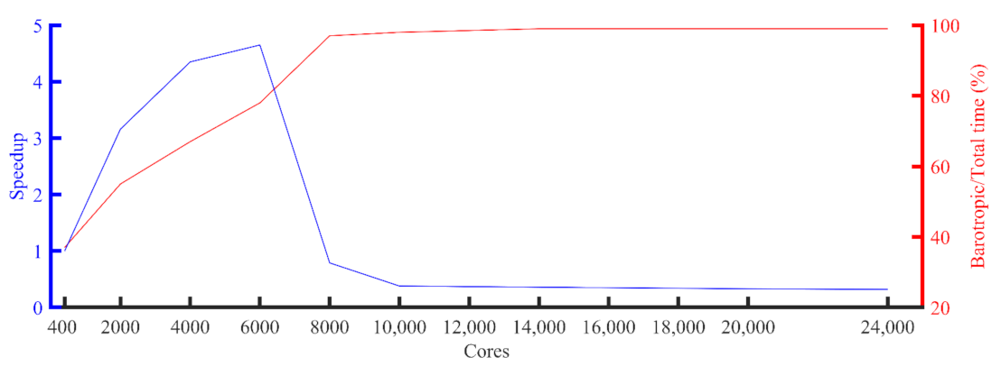
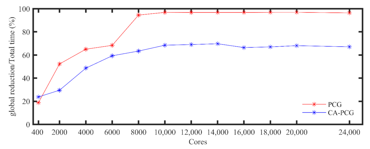
3.2. Performance of the NEMO Model Using the CA-PCG Solver

Before investigating the performance of the model using the CA-PCG solver, it was important to compare the global reductions before and after optimization. As shown in Figure 5, the percentage of global reductions increased with the number of GYRE_PCG experiment processes. When more than 8000 processes were used, the execution time of the global reduction increased to more than 94.5% of the total execution time and could even reach 99.9% when using 24,000 processes. However, the execution time was reduced to 63.4% when using the CA-PCG solver. The ratio of the percentage of the global reductions in the two experiments was calculated (Figure 6). Almost all the ratios in the GYRE_CAPCG to GYRE_PCG experiment were less than 1, except when using 400 processes, due to the increase in the calculation time after optimization. When using more than 8000 processes, the ratio was approximately 0.70. Thus, the CA-PCG solver was useful for reducing the operation of global reduction, especially when scaled to more than 8000 processes.
The total execution time considering different numbers of processes in both GYRE_PCG and GYRE_CAPCG is shown in Table 1. The total execution time decreased as the number of processes employed increased in the GYRE_PCG experiment when using less than 6000 processes, and the minimum time was 1510 s, which was due to the decrease in the cost of computation. However, it greatly increased to more than 18,000 s when using more than 10,000 processes because of the dramatic increase in global reduction. After comparing the total execution time for GYRE_PCG and GYRE_CAPCG, we found that the differences were not considered with less than 6000 processes. Sometimes the execution time in GYRE_CAPCG was longer than that in GYRE_PCG due to the increase in the required computation. However, as the model scaled to larger scales, especially more than 10,000 processes, the total execution time decreased to 4000–6000 s in GYRE_CAPCG, much faster than that in GYRE_PCG. After optimization, there was a 3.56–4.40-fold improvement at large scales, which effectively reduced the model simulation costs.
Next, we tested the overall performance of the NEMO model. The speedup was also greatly improved after optimization, especially at large scales (Table 1). With the PCG solver, the speedup relative to 400 processes was 4.65 times when using 6000 processes. However, the speedup decreased to less than 1.0 times when using more than 8000 processes, while in GYRE_CAPCG, the speedup was still greater than 1.0 times at large scales. After comparing the speedup in GYRE_PCG and GYRE_CAPCG (Figure 8), we found that the ratio of GYRE_CAPCG to GYRE_PCG was larger than 1 when using more than 6000 processes and reached 4.61 when using more than 10,000 processes, which demonstrates an efficient improvement.

4. Discussion and Conclusions

As the number of processors used has increased, the barotropic solver in the NEMO model has become the bottleneck for large-scale clusters. The most time-consuming part is solving elliptic equations, for which it is recommended that the PCG method is used in NEMO. In this work, we developed and implemented the CA-PCG method in the model to solve this problem. The results showed that the requirement of inner product operations decreased from each iteration to every eight iterations, which highly reduced the global reduction when using the newly developed CA-PCG solver. Thus, the execution time of the barotropic mode decreased effectively. Additionally, the speedup of NEMO after optimization was also better than that before optimization.
Above all, the optimization method could be useful in optimizing the NEMO model at large scales, as in this study. It should be noted that the main effect of the CA-PCG solver is reducing the cost of the global reduction during simulation. However, the architecture of the cluster, such as the bandwidth and the resolution of the experiment will impact the execution time of global reduction and can further influence the efficiency of the CA-PCG solver. To further evaluate the new barotropic solver’s effectiveness, the optimized model should be tested on different clusters, including Heterogeneous System Architecture. Moreover, the accuracy of the results after optimization was only validated using small-scale simulation due to computation and storage limitations. Exploring different grid resolutions, particularly large-scale ones, is critical and should also be validated in the future. Besides, it should also be noted that the distribution of the ensemble z-score biases shows a seasonal variation (Figure 4), which also needs further analysis.
The experience gained from the NEMO model could benefit other OGCMs and even other ocean components in coupled models. In the Coupled Model Intercomparison Project phase 6 (CMIP6), approximately 25 climate models use NEMO as their ocean component (https://github.com/WCRP-CMIP/CMIP6_CVs/blob/master/CMIP6_source_id.json (accessed on 10 April 2021)). Climate models usually require numerous calculations and long integral times and need to be run on high-performance computing resources more than stand-alone ocean models do [20]. Therefore, the NEMO model’s high performance will benefit from simple ocean process simulation and climate models that use NEMO as their ocean component.

Author Contributions

Methodology, validation, analysis, and writing–original draft preparation, X.Y.; algorithm coding and description, S.Z. (Shan Zhou); numerical experiments, S.Z. (Shengchang Zhou); conceptualization, supervision, funding acquisition, and writing–review and editing, Z.S.; algorithm and numerical experiments’ suggestion, W.L. All authors discussed, read, edited, and approved the article. All authors have read and agreed to the published version of the manuscript.

Funding

This research was funded by the National Natural Science Foundation of China (nos. U1806205, 41906029, and 42022042) and the China–Korea Cooperation Project on Northwestern Pacific Climate Change and its Prediction.

Institutional Review Board Statement

Not applicable.

Informed Consent Statement

Not applicable.

Data Availability Statement

The data used within this study are the combination of the World Ocean Atlas 2009 and the Polar Science Center Hydrographic Climatology version 3 data, which can be obtained from the National Oceanographic Data Center (NODC) and Polar Science Center, respectively.

Acknowledgments

The authors are grateful to Junmin Lin and Zhe Wang for developing the algorithm.

Conflicts of Interest

The authors declare no conflict of interest.

Appendix A

The OGCMs solve the three-dimensional primitive equations, including Navier–Stokes equation, static equilibrium equation, continuity equation, temperature and salinity conservation equation, and state equation. The equations governing the dynamics of coastal circulation contain fast-moving, external gravity waves, and slow-moving, internal gravity waves. It is desirable in terms of computer economy to separate the vertically integrated equations (barotropic mode) from the vertical structure equations (baroclinic mode). This technique, known as mode splitting, permits the calculation of the free surface elevation with little sacrifice in computational time by solving the velocity transport separately from the three-dimensional calculation of the velocity and the thermodynamic properties. The split-explicit free surface formulation used in the NEMO model follows the one proposed by [21]. The general idea is to solve the free-surface equation and the associated barotropic velocity equations with a smaller time step than Δt, which is the time step used in the baroclinic mode for the three-dimensional prognostic variables (Figure A1).
The barotropic mode solves the following depth-integrated equations:
U ¯ t = f k × U ¯ g η c H + η U ¯ + G ¯
η t = · H + η U ¯ + P E
where U ¯ is the depth-integrated barotropic velocity, η is the sea surface height, f is the Coriolis parameter, and g is the acceleration of gravity. G ¯ is a forcing term held constant, containing coupling term between modes, surface atmospheric forcing, and slowly varying barotropic terms not explicitly computed to improve efficiency. The third term on the right-hand side of Equation (A1) represents the bottom stress. H represents the depth of the ocean. P and E represent the precipitation and evaporation, respectively.
Time filtering is eventually applied to barotropic quantities to avoid aliasing of fast barotropic motions into three-dimensional equations. When the filtered sea surface height option is used, the momentum equation’s force is solved implicitly. Thus, an elliptic equation, which is solved using the PCG solver in the NEMO model, is formulated.
Figure A1. The split time stepping is used in the model. The m represents the time of the barotropic step, and M is the total number of steps among each baroclinic step.
Jmse 09 00421 g0a1

Appendix B

Algorithm A1. Preconditioned conjugate gradient (PCG) [22].
Required: Coefficient matrix A , which is a definite positive symmetric matrix, preconditioner M   (diagonal matrix of the diagonal elements of A), initial guess value x 1 and vector b associated with grid block A i , j
1. Initialization: Given initial guess x 0 ,
2.  d 1 = 0 ,   z 1 = 0 , σ 1 = 0 ,   γ 1 = 1 ,   k = 0  /* initial the value */
3.  r 1 = M 1 ( b Ax 1 )          /* preconditioner */
4. For k = 1 : k max until convergence
5.  s k = Ar k                /* matrix-vector multiplication */
6.  γ k = rr k = r k T Mr k          /* inner product, global reduction */
7.  δ k = r k T Ms k             /* inner product, global reduction */
8.  β k = γ k / γ k 1
9.  d k = r k + β k d k 1
10.  z k = s k + β k z k 1
11.  σ k = δ k β k 2 σ k 1
12.  α k = γ k / σ k
13.  x k = x k 1 + α k d k         /* update vector */
14.  r k = r k 1 α k z k         /* update vector */
15. Update_Halo( r k )         /* boundary communication*/
16. End for              /* the result is x k */
NEMO divides the global domain into blocks and distributes them to the processes. Each process computes the only evolution procedures related to the grid points in its block and maintains a halo region to update data with its neighbors [9]. The following assumptions were made:
  • N × N is the global domain size.
  • The global domain is divided into m x m blocks with a size of n x n ( n = N / m ).
  • The p = m × m processes occur, and each process corresponds to exactly one grid block. Then, the total time of the barotropic mode is the execution time of the PCG solver on each block.
  • K is the iteration number.
Then, for each iteration, t comp is the cost of the computation, t b is the cost of the boundary updating, and t g is the cost of the global reduction. Below is a detailed estimation of these components.
(1) Computational cost
For Algorithm A1, the computational cost, t comp , contains three parts:
  • Step 5, with a total of 9n operations from one matrix-vector multiplication (MVM).
  • Steps 6 and 7, with a total of 6n operations, from two vector–vector multiplication (VVMs) for inner products, two additional inverse operations of the preconditioner, which has the same cost as the preconditioner (for the diagonal preconditioner, its operation number is n), and two masking operations for land point exclusion.
  • Steps 10, 11, 13, and 14, with a total of 4n operations, from four vector-scaling operations.
The total cost can be expressed as:
t c o m p = K 9 n 2 + 6 n 2 + 4 n 2 σ = 19 N 2 p σ K
where σ is the execution time per floating-point operation. If the domain size N is constant, t comp decreases to a lower bound of zero when the number of processes increases.
(2) Communication cost
There are two kinds of communication in the solver. The first one is from the boundary update. After MVM and nondiagonal preconditioning, a boundary update occurs in the halo regions for each process, which requires one or more boundary layers to be updated. In NEMO, since each process covers one block and one additional halo layer is used, only one boundary update is needed per iteration. The total boundary updating cost depends on the data volume of the halo regions and network latency. When the halo size is 1, the data volume in each boundary is n, and there are four boundaries for each block (east, west, north, and south). Then, the total boundary updating cost for each iteration satisfies:
  t b = K 4 θ + 4 n ε = K 4 θ + 4 N p ε
where θ is the point-to-point communication latency per message and ε is the transfer time per floating-point datum. The boundary updating time also decreases as the number of processes increases but has a lower limit of 4 θ . The second communication cost is due to global reduction and can be estimated with a similar method. There are two global reductions per iteration, each of which results in a reduction in computing time and communication latency. Considering a binomial tree, the communication latency cost should be δ log 2 p [10]. Then, the global reduction execution time can be regarded as:
t g = K 2 N 2 p σ + θ l o g 2 p
When the process number p increases, the cost of the computing time should decrease, and the cost of the communication latency should increase monotonically. Combining computational costs together with boundary updating and global reduction costs, the execution time of one step for NEMO PCG can be described as:
t p c g = t c o m p + t c o m m ) = ( t c o m p + t b + t g   = K 21 N 2 p σ + 4 N p ε + 4 + l o g 2 p θ
where K is constant regardless of how many processes are used [23].
Equation (A6) shows that the more processes used, the less time is required for computation and boundary updating. However, the time required for global reduction increases with the number of processes. Therefore, when the process number exceeds a certain limit, the total time of the NEMO PCG solver will increase monotonically and become dominant.

Appendix C

Algorithm A2. Communication-avoiding Krylov subspace method with a PCG (CA-PCG)
CA-PCG consists of a two-level nested loop (k,j), outer loop indexed by k, and inner loop index j 1 , , s , given initial PCG vectors p sk + 1 , z sk + 1 , and x sk + 1 :
outer loop: prepare the required info for iterations over p sk + j and z sk + j , x sk + j
inner loop: update the PCG vectors with their coordinates in the Krylov subspace
    K k A , v = span v , Av , A 2 v , , A k 1 v
1. Initialization: Given initial guess x 0 and set residual r 1 = b Ax 1 , outer   loop   index   k = 1 ,
2.  z 1 = p 1 = M 1 r 1         /* preconditioner */
3. For k = 1 : k max / s , until convergence done
4. /* construct and compute P k , Z k , a polynomial of degree j with ρ j τ and p sk + 1 ,   z sk + 1 */ /* matrix-vector multiplication */ P k = [ ρ 0 M 1 A p sk + 1 , , ρ s M 1 A p sk + 1 ] ,   sat . span P k = K s + 1 M 1 A , p sk + 1 Z k = [ ρ 0 M 1 A z sk + 1 , , ρ s 1 M 1 A z sk + 1 ] ,   sat .   span Z k =   K s M 1 A , z sk + 1
5.  Update _ halo V k         /* boundary communication */
6. Compute Gram matrix G k = V k T M V k /* inner product with global reduction */
7. Assemble B k from ρ j τ , which is a change basis matrix, with all 0 in columns s + 1 and 2s + 1
8. Initial short vector p k , j = 1 , 0 2 s T , z k , j = 0 s + 1 , 1 , 0 s + 1 T ,   x k , j = 0 2 s + 1 T
9.  For   j = 1 , s   do         /* s = 8 in this paper */
10. /* inner product, G k is ready, no global reduction */
α k , j = z k , j T G k z k , j / p k , j T G k B k p k , j
11.  x k , j + 1 = x k , j + α k , j p k , j           /* update short vector */
12.  z k , j + 1 = z k , j α k , j B k p k , j         /* update short vector */
13. /* inner product, G k is ready, no global reduction */
β k , j = z k , j + 1 T G k z k , j + 1 / z k , j T G k z k , j
14.  p k , j + 1 = z k , j + 1 + β k , j p k , j         /* update short vector */
15.  End   for                   /* inner loop end */
16.  p k , j = V k   p k , j , z k , j = V k   z k , j , x k , j = V k   x k , j + x k , 1   /* update long vectors*/
17.  Update _ halo x k , j         /* boundary communication */
18.  End   for               /* outer loop end, the result is x k */
Regarding B k , ρ j τ satisfies the three-term recurrence via
ρ 0 τ = 1 , ρ 1 τ = τ θ 0 ρ 0 τ / γ 0 , and ρ j τ = ( τ θ j 1 ρ j 1 τ σ j 2 ρ j 2   τ / γ j 1 .
  In this paper, the monomial bases were used, so γ j = 1   and   θ j = σ j = 0 .
In the CA-PCG algorithm, all of the iterations are divided into two layers of loops. In the outer loop, global reductions are still needed to obtain the Gram matrix [13], which can be used in the inner loop. Since we used the same preconditioner as that used for PCG, the convergence rate will not change, and the iteration number K should be the same. If s is the inner loop count, then the outer loop count will be K/s, which means one global reduction is needed after every s iterations. Since the inner loop count increases, the optimization efficiency will be improved, but the computational accuracy will decrease. We found that eight inner loop counts could meet both optimization efficiency and computational accuracy after multiple tests. Then the inner loop count s was set as eight in this study. However, in the PCG algorithm, one global reduction was needed after each iteration step. Thus, the amount of global reduction was reduced to 1/8 of that in the PCG algorithm. Notably, even though the global communication cost was highly reduced, the computational cost was increased compared to the PCG algorithm.
Assuming that the complexity of PCG is N comp , then CA-PCG is 2 s + 1 2 N comp , which comes from steps 4, 10, 11, 12, 13, 14, and 16 in Algorithm A2, especially step 4. To reduce the computation cost of CA-PCG, we implemented optimizations to reduce the computation complexity to 6s* N comp . The hotspots of CA-PCG were the basic operation in step 4 and the Gram matrix operation in step 6, while the costs of the inner iterations were negligible (from steps 10 to 14). The count of MVM in step 4 was 2s − 1, approximately twice that of the PCG iterations, which could be amortized by data parallelization. The complexity of the inner production in step 6 was (2s + 1)2 with a naive implementation or approximately (2s + 1)2/2 by taking the symmetric property of matrix A and M−1. However, the computational cost was still high and could be reduced further. With the choice of monomial basis and diagonal matrix M−1, the element in the Gram matrix Gk(i,j) was ( p s k + 1 or z s k + 1 ) by M(M−1A)i−1(M−1A)j−1 by (psk+1 or zsk+1). After the argument, Gk(i1,j1) and Gk(i2,j2) were equal, given that they were in the same submatrix (e.g., P k MPk) and i1+j1 = i2+j2. As a result, the counts of the inner products needed for submatrices P k MPk, P k MZk, and Z k MZk were 2s + 1, 2s, and 2s − 1, respectively. In total, the computational complexity of the inner products was reduced to 6s at the algorithmic level compared to 2s in the corresponding PCG iterations.
The details about the computational and communication cost estimation after optimization are provided here. The communication cost comes from the boundary updating in steps 5 and 17 and the global reduction cost of step 6. Thus, we can obtain the following:
t c o m p = 19 K 6 s N 2 p σ
  t b = K s 8 θ + 8 n ε = K s 8 θ + 8 N p ε
t g = 2 s N 2 p σ + θ l o g 2 p K s = 2 K N 2 p σ + K s θ l o g 2 p
t c a p c g = 19 K 6 s + 2 K N 2 p σ + K s 8 N p ε + K s 8 + l o g 2 p θ
According to the impact of the processor number p, we divided t capcg into two parts, F capcg 1 and F capcg 2 :
F c a p c g 1 =   19 K 6 s + 2 K N 2 p σ + K s 8 N p ε
F c a p c g 2 = K s 8 + l o g 2 p θ
Implementing the same operation on Equation (A6), we can convert Equation (A6) into:
t p c g = F p c g 1 + F p c g 2 ,
where:
F p c g 1 =   21 K N 2 p σ + K 4 N p ε ]
F p c g 2 =   K 4 + l o g 2 p θ ]
where s is the inner loop count. As shown in Equation (A12), the cost of global communication will decrease as s increases in CA-PCG. However, s has a limit value, which depends on the basis we choose in the algorithm. Since the s monomial basis was used in this paper, the maximum value of s should be 8, or the solver cannot achieve convergence regardless of the iteration number [24].
From Equations (A11) and (A13), we can determine that the computational cost of the CA-PCG algorithm is greater than that of the PCG algorithm. However, for a certain workload, as p increases, there will be a lower limit of zero for computational cost. From Equations (A12) and (A14), we found that as p increases, the global reduction in CA-PCG reduces to approximately 1 s of that of the PCG algorithm. Moreover, we could also predict that there is a certain value p inf for the process number. When p < p inf , the computational cost is dominant, and the performance of the CA-PCG method is even worse than that of the PCG method. However, when p > p inf , the communication bottleneck due to the global reductions becomes considerable, and the CA-PCG method becomes very effective in reducing the communication cost, compared to the PCG method. Thus, the scalability is improved effectively with the CA-PCG solver.
Even though the CA-PCG solver can improve the performance of NEMO, correctness and accuracy should be ensured. After optimization, the solution of the barotropic solver should be the same or very close. In both the PCG and CA-PCG solver, the solution is an approximate value that can satisfy the condition of convergence (Algorithm A1, A2). If the solution of the CA-PCG solver is correct, it should also make the PCG solver achieve convergence. Thus, we used the most direct method to verify the correctness of the result. After applying the solution of the CA-PCG solver as the initial guess value of the PCG solver, we found that only one step iteration was needed to reach convergence. Then, the solution of the new solver CA-PCG can be recognized as the correct solution of this elliptic equation in the barotropic mode of NEMO.

Appendix D

Table A1. Description of the parallel platform.
CPU2*Intel Xeon Scalable Cascade Lake 6248 (2.5 GHz, 20 Cores)
L3 cache27.5 MB
Memory12 × Samsung 16 GB DDR4 ECC REG 2666
Interconnect (Network)Intel OmniPath 100 Gbps
StorageLustre (NVMe)
BIOS settings4.1.05
OS/kernel3.10.0-1062.el7.x86_64

References

  1. Chassignet, E.P.; Xu, X. Impact of Horizontal Resolution (1/12° to 1/50°) on Gulf Stream Separation, Penetration, and Variability. J. Phys. Oceanogr. 2019, 47, 1999–2021. [Google Scholar] [CrossRef]
  2. Qiao, F.; Zhao, W.; Yin, X.; Huang, X.; Liu, X.; Shu, Q.; Wang, G.; Song, Z.; Li, X.; Liu, H.; et al. A Highly Effective Global Surface Wave Numerical Simulation with Ultra-High Resolution. In Proceedings of the SC16: International Conference for High Performance Computing, Networking, Storage and Analysis, Salt Lake City, UT, USA, 13–18 November 2016; pp. 46–56. [Google Scholar]
  3. Zhao, W.; Song, Z.Y.; Qiao, F.L.; Yin, X.Q. High efficient parallel numerical surface wave model based on an irregular quasi-rectangular domain decomposition scheme. Sci. China Earth Sci. 2014, 44, 1049–1058. [Google Scholar] [CrossRef]
  4. Cohn, S.E.; Dee, D.; Marchesin, D.; Isaacson, E.; Zwas, G. A fully implicit scheme for the barotropic primitive equations. Mon. Weather Rev. 1985, 113, 641–646. [Google Scholar] [CrossRef] [Green Version]
  5. Dukowicz, J.K.; Smith, R.D. Implicit free-surface method for the Bryan-Cox-Semtner ocean model. J. Geophy. Res. Ocean. 1994, 99, 7991–8014. [Google Scholar] [CrossRef]
  6. Concus, P.; Golub, G.H.; O’Leary, D.P. Numerical solution of nonlinear elliptic partial differential equations by a generalized conjugate gradient method. Computing 1978, 19, 321–339. [Google Scholar] [CrossRef]
  7. Concus, M. On computingINV block preconditionings for the conjugate gradient method. BIT 1986, 26, 493–504. [Google Scholar] [CrossRef]
  8. Smith, R.; Jones, P.; Briegleb, B.; Bryan, F.; Danabasoglu, G.; Dennis, J.; Dukowicz, J.; Eden, C.; Fox-Kemper, B.; Gent, P.; et al. The Parallel Ocean Program (POP) Reference Manual; Tech. Rep. LAUR-10-01853; Los Alamos National Laboratory: Los Alamos, NM, USA, 2010; p. 141. [Google Scholar]
  9. Madec, G. NEMO Ocean Engine. In Note du Pole de Modelisation; Institut Pierre-Simon Laplace: Paris, France, 2008; p. 27. [Google Scholar]
  10. Xu, S.; Huang, X.; Oey, L.Y.; Xu, F.; Fu, H.; Zhang, Y.; Yang, G. POM.gpu-v1.0: A GPU-based Princeton Ocean Model. Geosci. Model. Dev. 2015, 8, 2815–2827. [Google Scholar] [CrossRef] [Green Version]
  11. Hu, Y.; Huang, X.; Baker, A.; Tseng, Y.; Bryan, F.; Dennis, J.; Yang, G. Improving the scalability of the ocean barotropic solver in the community earth system model. In Proceedings of the International Conference for High Performance Computing, Networking, Storage and Analysis, Austin, TX, USA, 15 November 2015; pp. 1–12. [Google Scholar]
  12. Madec, G.; Delecluse, P.; Imbard, M.; Levy, C. Opa 8 ocean general circulation model reference manual. Tech. Rep. 1998, 11, 91. [Google Scholar]
  13. Carson, E. Communication-Avoiding Krylov Subspace Methods in Theory and Practice. Ph.D. Thesis, University of California, Berkeley, CA, USA, 2015. [Google Scholar]
  14. Antonov, J.I.; Seidov, D.; Boyer, T.P.; Locarnini, R.A.; Johnson, D.R. World Ocean. Atlas 2009 Volume 2: Salinity; Levitus, S., Ed.; NOAA Atlas NESDIS 69; U.S. Government Printing Office: Washington, DC, USA, 2010; p. 184.
  15. Locarnini, R.; Mishonov, A.; Antonov, J.; Boyer, T.; Garcia, H.; Baranova, O.; Zweng, M.; Johnson, D. World Ocean. Atlas 2009, Volume 1: Temperature; NOAA Atlas NESDIS 61; U.S. Government Printing Office: Washington, DC, USA, 2010; p. 182.
  16. Steele, M.; Morley, R.; Ermold, W. PHC: A global ocean hydrography with a high quality Arctic Ocean. J. Clim. 2001, 14, 2079–2087. [Google Scholar] [CrossRef]
  17. Griffies, S.M.; Biastoch, A.; Böning, C.; Bryan, F.; Jianjun, Y. Coordinated ocean-ice reference experiments (COREs). Ocean. Modell. 2009, 26, 1–46. [Google Scholar] [CrossRef]
  18. Large, W.G.; Yeager, S.G. The global climatology of an interannually varying air–sea flux data set. Clim. Dyn. 2009, 33, 341–364. [Google Scholar] [CrossRef]
  19. Baker, A.; Xu, H.; Dennis, J.; Levy, M.; Nychka, D.; Mickelson, S.; Edwards, J.; Vertenstein, M.; Wegener, A. A methodology for evaluating the impact of data compression on climate simulation data. In Proceedings of the 23rd International Symposium on High-Performance Parallel and Distributed Computing, Vancouver, BC, Canada, 23–27 June 2014; pp. 203–214. [Google Scholar]
  20. Wang, Y.; Hao, H.; Zhang, J.; Jiang, J.; He, J.; Ma, Y. Performance optimization and evaluation for parallel processing of big data in earth system models. Cluster Comput. 2017, 22, 2371–2381. [Google Scholar] [CrossRef]
  21. Shchepetkin, A.F.; McWilliams, J.C. The regional oceanic modeling system (roms)—a split-explicit, free-surface, topography-following-coordinate oceanic model. Ocean. Model. 2005, 9, 347–404. [Google Scholar] [CrossRef]
  22. Eisenstat, S.C. Efficient Implementation of a Class of Preconditioned Conjugate Gradient Methods. Siam J. Sci. Comput. 1981, 2, 1–4. [Google Scholar] [CrossRef] [Green Version]
  23. Hu, Y.; Huang, X.; Wang, X.; Fu, H.; Xu, S.; Ruan, H.; Xue, W.; Yang, G. A scalable barotropic mode solver for the parallel ocean program. In Proceedings of the Euro-Par 2013 Parallel Processing, Aachen, Germany, 26–30 August 2013; Springer: Berlin/Heidelberg, Germany, 2013; pp. 739–750. [Google Scholar]
  24. Hoemmen, M. Communication-Avoiding Krylov Subspace Methods. Ph.D. Thesis, University of California, Berkeley, CA, USA, 2010. [Google Scholar]
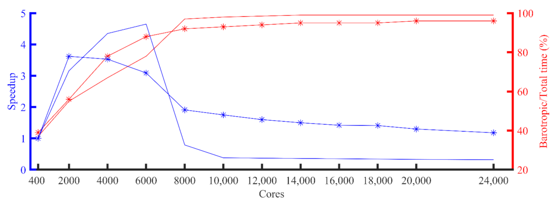
Figure 1. Speedup of the 5-km Nucleus for European Modelling of the Ocean (NEMO) experiment using the preconditioned conjugate gradient (PCG) solver (blue line) and the percentage of the barotropic time of the total execution time (red line). The baseline of the speedup is the running time corresponding to 400 processes.
Jmse 09 00421 g001
Figure 2. Percentage of the global reduction (MPI_Allreduce) time of the total execution time in the 5-km NEMO experiment with the PCG solver.
Jmse 09 00421 g002
Figure 3. Flow chart of the experiments in this study. The experiments were designed in order of step1, step2, step3, and step4.
Jmse 09 00421 g003
Figure 4. Z-score biases of temperature in ensemble run (grey lines) and the communication-avoiding Krylov subspace method with a preconditioned conjugate gradient (CA-PCG) solver experiment (black line). The dashed line represents the mean value of the z-score biases of all the ensemble runs.
Jmse 09 00421 g004
Figure 5. Percentages of the global reduction (MPI_Allreduce) time of the total execution time in 5-km Nucleus for European Modelling of the Ocean (NEMO) experiments using the preconditioned conjugate gradient (PCG) (blue line) and CA-PCG (red line) solvers.
Jmse 09 00421 g005
Figure 6. Ratio of the percentage of the global reduction (MPI_Allreduce) time of the total execution time determined using the CA-PCG and PCG solvers. In particular, the barotropic mode in GYRE_PCG accounted for approximately 97–99% of the total execution times when scaled to more than 8000 processes (Figure 7). After using the new CA-PCG solver, the percentage decreased slightly to approximately 92–96%. Even though the reduction in the percentage does not seem notable, the execution time of the barotropic mode decreased from more than 17,000 s to less than 6000 s (figure not shown).
Jmse 09 00421 g006
Figure 7. Speedup of 5-km NEMO experiments using the PCG (solid blue line) and CA-PCG (blue solid-star line) solvers. Percentages of the barotropic time of the total execution time using the PCG (solid red line) and CA-PCG (red solid-star line) solvers.
Jmse 09 00421 g007
Figure 8. Ratio of the speedup of the NEMO model using the CA-PCG and PCG solvers (blue line) and the ratio of the percentage of the barotropic time of the total execution time using the CA-PCG and PCG solvers (red line).
Jmse 09 00421 g008
Table 1. Execution time for the high-resolution experiments.
Number of ProcessesGYRE_PCG (s)SpeedupGYRE_CAPCG (s)Speedup
40070251.0071961.00
200022213.1619873.62
400016144.3520353.53
600015104.6523293.09
800088410.7937621.91
10,00018,0760.3841091.75
12,00018,7840.3744991.60
14,00019,4930.3647891.50
16,00020,0050.3550671.42
18,00020,4700.3451141.41
20,00020,9360.3355391.30
24,00021,7370.3261041.18
Publisher’s Note: MDPI stays neutral with regard to jurisdictional claims in published maps and institutional affiliations.

