Output Feedback Cooperative Dynamic Positioning Control for an Unactuated Floating Object Using Multiple Vessels

Abstract

This paper proposes an output feedback cooperative dynamic positioning control scheme for an unactuated floating object using multiple vessels under model uncertainties and environmental disturbances. The floating object is connected to multiple vessels through towlines. At first, nonlinear extended state observers are developed for the floating object and vessels to reconstruct the unmeasured velocity and to estimate the model uncertainties and disturbances. Second, observer-based controllers are designed for the floating object and vessels to drive the floating object to track the reference signal and to achieve the cooperative control of multiple vessels, respectively. The salient features of the proposed control scheme are presented as follows. Firstly, by design the object controller, the tracking performance of the object is improved. Secondly, according to the required force of the floating object, the time-varying formation of vessels is obtained by using the towline attachment geometry of the floating object, control allocation and a towline model. It is shown that all signals in closed-loop system are bounded via Lyapunov analysis. Simulation study is carried out to verify the effectiveness of proposed control method.

1. Introduction

Dynamic positioning (DP) operation for floating objects such as barges, offshore platforms and unactuated vessels, is an important application in marine industry while these floating objects usually are not designed, or not able to generate the necessary control forces to achieve DP operation. Cooperative DP using a fleet of vessels is a feasible solution for maneuvering the floating objects.

Considering the floating object is connected to multiple vessels through towlines, there are some studies reported in the literature. In [1,2], an underwater vehicle connected with an unmanned surface vehicle using umbilical cable is studied. But the underwater vehicle and the surface vehicle are fully actuated. Considering the floating object is unactuated, an automatic load maneuver controller is proposed using linear consensus control law in [3], where the dynamic model of vessels is simplified as a second-order linear model. However, the tracking performance of the floating object is not guaranteed. A time-varying formation based distributed model predictive control approach for a floating object transport with multiple vessels is proposed in [4]. But the environmental disturbances are not considered.

The tracking control precision of marine vessels is affected by environmental forces due to wind, waves and ocean currents. Some control strategies have been proposed to compensate the environmental disturbances. In [5,6,7], disturbance observers are used to estimate the time-varying disturbances. But the model uncertainties are not considered. Robust sliding mode controllers are designed for position-keeping of an underwater vehicle under ocean currents and model uncertainties in [8,9]. However, all states in above research are needed in the control design process. In practice, position-heading of the marine vessels are easily available using global satellite navigation system and gyro, while the velocity may not be measured. Therefore, it is necessary to investigate distributed control problem in the absence of velocity measurements. Nonlinear state observers [10,11] are proposed for DP ships to estimate the disturbances and reconstruct the velocity information. These proposed state observers requiring the model parameters are known. Some neural network or fuzzy logical based output feedback controllers are designed in [12,13,14]. But, these proposed adaptive observers or proposed observer-based controllers need to adjust too many parameters, which is not convenient for real application.

Motivated by the above analysis, this paper studies the cooperative DP control for an unactuated floating object that connected to multiple DP vessels using towlines under unavailability of velocity measurements, model parameter uncertainties and environmental disturbances, and proposes an output feedback cooperative DP control method. Nonlinear extended state observers (NESOs) for the floating object and vessels are employed to reconstruct the unmeasured velocity as well as estimate the model uncertainties and environmental disturbances. The NESOs only need to adjust one parameter. Then, NESO-based controllers are designed for the unactuated floating object and multiple DP vessels to realize tracking the reference signal of the unactuated floating object and cooperative tracking the unactuated floating object of multiple vessels, respectively. Especially, according to the required force of the floating object, the desired time-varying formation of vessels is determined by using the towline attachment geometry of the floating object, control allocation and a towline model. In addition, second order linear tracking differentiators are introduced to estimate the derivations of the complex virtual control laws.

The main contributions are summarized as follows.

• Compared with the proposed method in [3], where the floating object tracking performance is not guaranteed, the proposed method in this paper can improve the tracking performance of the floating object.
• Compared with the proposed method in [4], where the disturbances and model parameter uncertainties are not considered, this paper simultaneously considers the disturbances and model parameter uncertainties.
• According to the required force of the floating object, the desired time-varying formation of vessels is determined by using the towline attachment geometry of the floating object, control allocation and a towline model.
• Second order linear tracking differentiators are introduced to estimate the derivations of the complex virtual control laws.

This paper is organized as follows: Section 2 describes some necessary preliminaries and states cooperative DP control problem. In Section 3, the control method is designed and the stability of the overall system is analyzed. It is proved that all signals in the closed-loop system are uniformly ultimately bounded. A simulation study using an unactuated platform and four vessels is given to verify the effectiveness of the proposed control method in Section 4. Section 5 concludes this paper.

Notations:The following notations will be used throughout the paper. $\left|·\right|$ indicates the absolute value of a scalar. $\overline{\lambda }\left(·\right)$ and $\underline{\lambda }\left(·\right)$ indicate the maximum and minimum eigenvalue of a square matrix, respectively. $∥·∥$ indicates a Euclidean norm. ${\mathbb{R}}^{n\times m}$ and ${\mathbb{R}}^n$ are $n\times m$ real matrix and $n\times 1$ real vector. $I_n$, $0_n$ and $0_{m\times n}$ are $n\times n$ identify matrix, $n\times n$ zero matrix and $m\times n$ zero matrix. $\mathrm{diag}\left\{a_j\right\}$ denotes a block-diagonal matrix, where $a_j$ is the jth diagonal element. ${\left(·\right)}^{-1}$ and ${\left(·\right)}^T$ indicate the inverse and transpose of a matrix, respectively. $C_s(·)$ and $S_n(·)$ denote $cos(·)$ and $sin(·)$, respectively. ⊗ denotes the Kronecker product of matrix.

2. Preliminaries and Problem Formulation

2.1. Graph Theory

The graph theory is used to describe the communication topology among four vessels. An undirected graph $\mathcal{G}=\left\{{\mathcal{V}}_{\mathcal{G}},\mathcal{E}\right\}$ consists of a node set ${\mathcal{V}}_{\mathcal{G}}=\{1,2,3,4\}$ and an edge set $\mathcal{E}=\left\{\left(i,j\right)\in {\mathcal{V}}_{\mathcal{G}}\times {\mathcal{V}}_{\mathcal{G}}\right\}$. The element $\left(i,j\right)\in \mathcal{E}$ denotes an edge that the jth node can access to the information of the ith node. An adjacency matrix is defined as $\mathcal{A}=\left[a_{ij}\right]\in {\mathbb{R}}^{n\times n}$, where $a_{ij}=1$, if $\left(j,i\right)\in \mathcal{E}$ and $i\ne j$; otherwise $a_{ij}=0$. The Laplacian matrix $\mathcal{L}$ associated with the undirected graph $\mathcal{G}$ is defined as $\mathcal{L}=\mathcal{D}-\mathcal{A}$, where $\mathcal{D}$ is the degree matrix of the graph and defined as $\mathcal{D}=\mathrm{diag}\left\{d_1,\dots ,d_n\right\}$ with $d_i={\sum }_{j=1}^4{a}_{ij}$. If there exists one path between every pair of nodes, the undirected graph $\mathcal{G}$ is connected. A diagonal matrix ${\mathcal{A}}_0=\mathrm{diag}\left\{a_{i0}\right\}$ is introduced to describe the communication between the floating object and the ith vessels, where $a_{i0}=1$, if the ith vessel can obtain the information from object, $a_{i0}=0$, otherwise. Further, the relationship of communication between the floating object and vessels is defined as a matrix $\mathcal{H}=\mathcal{L}+{\mathcal{A}}_0$.

Assumption 1.

There exists at least one directed path from the floating object to all vessels.

2.2. Towline Model

In this paper, considering the mass and the elasticity of the towline, a catenary model is used as towline model [15]

$$T_H=\left(D_H-2\frac{T_H}{\sigma }{sinh}^{-1}\left(\frac{\sigma L_R/2}{T_H}\right)\right)\frac{EA}{L_R},$$

(1)

where $T_R$ is the tension on the towline; $T_H$ is the tension in horizontal direction; $D_H$ is the horizontal position between two ends of the towline; $L_R$ is the length of the towline; $\sigma$ is the weight of the towline per unit length; E and A are the Young’s modulus and the cross-sectional area of the towline, respectively.

2.3. Problem Formulation

This paper considers the cooperative DP control for an unactuated floating object that connected with four vessels using towlines. The geometric configuration is shown in Figure 1. According to [16], the dynamic model of the ith vessel is expressed as

$$\left\{\begin{array}{c}{\dot{\eta }}_i=R\left({\psi }_i\right){\upsilon }_i,\hfill \\ M_i{\dot{\upsilon }}_i+D_i{\upsilon }_i={\tau }_i+{\tau }_H^i+{\tau }_d^i,\hfill \end{array}\right.$$

(2)

where ${\eta }_i={\left[x_i,y_i,{\psi }_i\right]}^T\in {\mathbb{R}}^{3\times 3}$ is the position and heading vector defined in the earth fixed frame $X_E{O}_E{Y}_E$ (See Figure 1); ${\upsilon }_i={\left[u_i,v_i,r_i\right]}^T\in {\mathbb{R}}^{3\times 3}$ is the velocity vector in the body fixed frame $X_{Bi}{O}_{Bi}{Y}_{Bi}$; $M_i\in {\mathbb{R}}^{3\times 3}$ the inertia matrix, which is symmetrical, positive definite and ${\dot{M}}_i=0$; $D_i\in {\mathbb{R}}^{3\times 3}$ is the unknown damping matrix. ${\tau }_i=\in {\mathbb{R}}^3$ is the control input vector; ${\tau }_H^i=B_i{T}_H^i$ is the horizontal force of towline acting on the ith vessels with $B_i=\left[C_s\left({\varphi }_i\right)\right.$, ${\left.S_n\left({\varphi }_i\right),0\right]}^T$ and $T_H^i$ being the horizontal tension on the ith towline; ${\tau }_d^i$ is the total environmental disturbances; $R\left({\psi }_i\right)\in {\mathbb{R}}^{3\times 3}$ is the rotation matrix that satisfies $\left|R\left({\psi }_i\right)\right|=1$, $R^T\left({\psi }_i\right)R\left({\psi }_i\right)=I_3$ and $\dot{R}\left({\psi }_i\right)=r_{i}SR\left({\psi }_i\right)$, where

$$R\left({\psi }_i\right)=\left[\begin{array}{ccc}{C}_s\left({\psi }_i\right)& -S_n\left({\psi }_i\right)& 0\\ S_n\left({\psi }_i\right)& C_s\left({\psi }_i\right)& 0\\ 0& 0& 1\end{array}\right],S=\left[\begin{array}{ccc}0& -1& 0\\ 1& 0& 0\\ 0& 0& 0\end{array}\right]$$

(3)

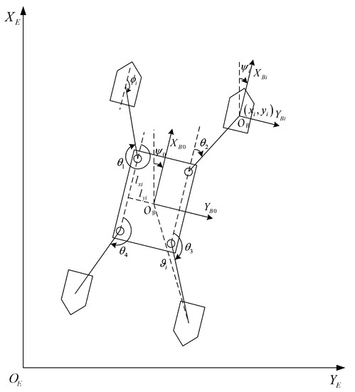
Figure 1. Configuration of four vessels and an unactuated floating object for cooperative DP.

To facilitate the following text written, ${\psi }_i$ is omitted without confusion, i.e., $R_i=R\left({\psi }_i\right)$ and $R_i^T=R^T\left({\psi }_i\right)$.

The dynamic model of the unactuated floating object is expressed as

$$\left\{\begin{array}{c}{\dot{\eta }}_0=R_0{\upsilon }_0,\hfill \\ M_0{\dot{\upsilon }}_0+D_0{\upsilon }_0={\tau }_0+{\tau }_d^0,\hfill \end{array}\right.$$

(4)

where ${\tau }_0=B_{0}T$ is the total control inputs generated by the connected towlines with

$$\begin{array}{cc}\hfill & T={\left[T_H^1,T_H^2,T_H^3,T_H^4\right]}^T,\hfill \\ \hfill & B_0={\left[\begin{array}{ccc}{C}_s\left({\theta }_1\right)\hfill & S_n\left({\theta }_1\right)& l_{x1}{S}_n\left({\theta }_1\right)-l_{y1}{C}_s\left({\theta }_1\right)\\ C_s\left({\theta }_2\right)\hfill & S_n\left({\theta }_2\right)& l_{x2}{S}_n\left({\theta }_2\right)-l_{y2}{C}_s\left({\theta }_2\right)\\ C_s\left({\theta }_3\right)\hfill & S_n\left({\theta }_3\right)& l_{x3}{S}_n\left({\theta }_3\right)-l_{y3}{C}_s\left({\theta }_3\right)\\ C_s\left({\theta }_4\right)\hfill & S_n\left({\theta }_4\right)& l_{x4}{S}_n\left({\theta }_4\right)-l_{y4}{C}_s\left({\theta }_4\right)\end{array}\right]}^T\hfill \end{array}$$

(5)

where ${\theta }_i$ and $l_{xi}$, $l_{yi}$ are the angles and moment arms defined in Figure 1. Other symbols are defined similar to the dynamic model of vessels.

Remark 1.

For practical application, the nominal inertial matrix $M_0$ and $M_i$ of the floating object and vessels can be obtained, while $D_0$ and $D_i$ may not be able to determine.

Definition 1.

The time-varying formation is defined as ${\Theta }_i=\left\{{\vartheta }_i\right\}$, where ${\vartheta }_i\in {\mathbb{R}}^3$ is the time-varying relative position between the floating object and the ith vessel (see Figure 1). Let ${\vartheta }_{ij}={\vartheta }_i-{\vartheta }_j$ be the time-varying relative deviation between the ith vessel and the jth vessel.

Remark 2.

Letting ${\eta }_{tow}^i,i=1,\dots ,4$ be the towed point on the floating object, the time-varying relative position between the floating object and the ith vessel is determined as

$${\vartheta }_i={\eta }_{tow}^i-{\eta }_0+d_H^i{B}_d^i$$

(6)

where $B_d^i={\left[C_s\left({\theta }_i+{\psi }_0\right),S_n\left({\theta }_i+{\psi }_0\right),{\delta }_i/d_H^i\right]}^T$ with ${\delta }_i$ being the designed constant and $d_H^i$ being the desired horizontal distance of the ith towline.

The control objective is to design a distributed output feedback control law for each vessel under model uncertainties and environmental disturbances such that:

O1.

The unactuated floating object can track the reference signal ${\eta }_d$, i.e.,

$$\underset{\mathrm{t}\to \infty }{lim}∥{\eta }_0-{\eta }_d∥\le o_1,$$

(7)

where $o_1>0$ is a small constant.

O2.

The vessels can track the floating object ${\eta }_0$ with time-varying formation, i.e.,

$$\underset{\mathrm{t}\to \infty }{lim}∥{\eta }_i-{\eta }_0-{\vartheta }_i∥\le o_2,$$

(8)

where $o_2>0$ is a small constant.

Assumption 2.

The reference signal ${\eta }_d$ is smooth enough such that ${\dot{\eta }}_d$ and ${\ddot{\eta }}_d$ exist and bound.

3. Control Design

3.1. NESOs Design for the Floating Object and Vessels

In this subsection, NESOs will be developed for the floating object and vessels to reconstruct the velocity and estimate the model uncertainties and environmental disturbances using the measured position-heading information. To design the NESOs, the floating object and vessels dynamic models are rewritten as

$$\left\{\begin{array}{c}{\dot{\eta }}_k=R_k{\upsilon }_k\hfill \\ {\dot{\upsilon }}_k=M_k^{-1}\left({\tau }_k+{\phi }_k\right)+{\varsigma }_k\hfill \end{array}\right.$$

(9)

where ${\phi }_0=0_{3\times 1}$, ${\phi }_i={\tau }_H^i,i=1,\dots ,4$, and ${\varsigma }_k$ is the lumped disturbance defined as ${\varsigma }_k=M_k^{-1}\left(-D_k{\upsilon }_k+{\tau }_d^k\right)$ with $k=0,1,\dots ,4$.

The following assumption is made for the NESOs design.

Assumption 3.

The lumped disturbances ${\varsigma }_k$ and its derivation ${\dot{\varsigma }}_k$ are bounded, i.e., there exist positive constants ${\overline{\varsigma }}_k$ and $q_k$, such that $∥{\varsigma }_k∥\le {\overline{\varsigma }}_k$ and $∥{\dot{\varsigma }}_k∥\le q_k$.

Let ${\widehat{\eta }}_k$ be the estimation of position ${\eta }_k$. Define the position estimation error as ${\tilde{\eta }}_k={\widehat{\eta }}_k-{\eta }_k$. Then, the NESOs are designed as [17]

$$\left\{\begin{array}{c}{\dot{\widehat{\eta }}}_k=-K_{ko1}{\tilde{\eta }}_k+R_k{\widehat{\upsilon }}_k\hfill \\ {\dot{\widehat{\upsilon }}}_k=-K_{ko2}{R}_k^T{\tilde{\eta }}_k+M_k^{-1}\left({\tau }_k+{\phi }_k\right)+{\widehat{\varsigma }}_k\hfill \\ {\dot{\widehat{\varsigma }}}_k=-K_{ko3}{R}_k^T{\tilde{\eta }}_k\hfill \end{array}\right.,$$

(10)

where $K_{ko1},K_{ko2},K_{ko3}\in {\mathbb{R}}^{3\times 3}$ are positive definite diagonal matrices and are selected as $K_{ko1}=3{\omega }_k{I}_3$, $K_{ko2}=3{\omega }_k^2{I}_3$ and $K_{ko3}={\omega }_k^3{I}_3$, respectively. ${\omega }_k$ is the designed observer bandwidth.

Defining ${\tilde{\upsilon }}_k={\widehat{\upsilon }}_k-{\upsilon }_k$ and ${\tilde{\varsigma }}_k={\widehat{\varsigma }}_k-{\varsigma }_k$, the error dynamics of the NESOs are derived as

$$\left\{\begin{array}{c}{\tilde{\eta }}_k=-K_{ko1}{\tilde{\eta }}_k+R_k{\tilde{\upsilon }}_k\hfill \\ {\dot{\tilde{\upsilon }}}_k=-K_{ko2}{R}_k^T{\tilde{\eta }}_k+{\tilde{\varsigma }}_k\hfill \\ {\dot{\tilde{\varsigma }}}_k=-K_{ko3}{R}_k^T{\tilde{\eta }}_k-{\dot{\varsigma }}_k\hfill \end{array}\right.$$

(11)

Collecting all the observer error states from (11) in a new vector $s_k=\mathrm{col}\left({\tilde{\eta }}_k,{\tilde{\upsilon }}_k,{\tilde{\varsigma }}_k\right)\in {\mathbb{R}}^9$, the observer error dynamics (11) is written compactly as

$${\dot{s}}_k=A_k{s}_k+B_k{\dot{\varsigma }}_k,$$

(12)

where $A_k=\left[\begin{array}{ccc}-K_{ko1}& R_k& 0_3\\ -K_{ko2}{R}_k^T& 0_3& I_3\\ -K_{ko3}{R}_k^T& 0_3& 0_3\end{array}\right]$ and $B_k={\left[0_3,0_3,-I_3\right]}^T$. $A_k$ depends on nonlinear term $R_k$. This will make the stability analysis of designed NESOs difficult. Therefore a transformation [18] is introduced

$${\chi }_k={\Xi }_k{s}_k,$$

(13)

where ${\Xi }_k=\mathrm{diag}\left\{R_k^T\right.$, $\left.I_3,I_3\right\}$. Using (13), the error dynamics (12) is rewritten as

$${\dot{\chi }}_k=\left(A_{k0}+r_k{S}_T\right){\chi }_k+B_k{\dot{\varsigma }}_k,$$

(14)

where $A_{k0}=\left[\begin{array}{ccc}-K_{ko1}& I_3& 0_3\\ -K_{ko2}& 0_3& I_3\\ -K_{ko3}& 0_3& 0_3\end{array}\right]$ and $S_T=\mathrm{diag}\left\{S^T,0_3,0_3\right\}$.

Then, the following Lemma holds.

Lemma 1. 

Consider the NESOs given by (10) under Assumption 3. The observer estimation errors $s_k$ is bounded, if the following inequalities hold

$$\left\{\begin{array}{c}{A}_{k0}^T{P}_k+P_k{A}_{k0}+P_k{B}_k{B}_k^T{P}_k+{\overline{r}}_k(S_T^T{P}_k+P_k{S}_T)\le -Q_k,\\ A_{k0}^T{P}_k+P_k{A}_{k0}+P_k{B}_k{B}_k^T{P}_k-{\overline{r}}_k(S_T^T{P}_k+P_k{S}_T)\le -Q_k,\end{array}\right.$$

(15)

where $P_k,Q_k\in {\mathbb{R}}^{9\times 9}$ are symmetric definite positive matrices, ${\overline{r}}_k$ is the upper bound of $r_k$.

Proof. 

See the Appendix A.1. □

3.2. The Tracking Control of the Floating Object

In this subsection, a NESO-based controller for the floating object is designed to guarantee the tracking performance of the floating object. The design process is shown as follows.

First, define the two tracking error vectors as

$$\left\{\begin{array}{c}{z}_{01}={\eta }_0-{\eta }_d\\ z_{02}={\widehat{\upsilon }}_0-{\alpha }_0\end{array}\right.$$

(16)

where ${\alpha }_0$ is a virtual law of the floating object to be designed. The time derivation of (16) is

$$\left\{\begin{array}{c}{\dot{z}}_{01}=R_0{\upsilon }_0-{\dot{\eta }}_d\hfill \\ {\dot{z}}_{02}=-K_{0o2}{R}_0^T{\tilde{\eta }}_0+M_0^{-1}{\tau }_0+{\widehat{\varsigma }}_0-{\dot{\alpha }}_0\hfill \end{array}\right.$$

(17)

In order to stabilize $z_{01}$ and $z_{02}$, the control law of the floating object is taken as

$$\left\{\begin{array}{c}{\alpha }_0=R_0^T\left(-K_{01}{z_0}_1+{\dot{\eta }}_d\right)\hfill \\ {\tau }_0=M_0\left(-K_{02}{z}_{02}+{\dot{\alpha }}_0-{\widehat{\varsigma }}_0-R_0^T{z}_{01}\right)\hfill \end{array}\right.$$

(18)

where $K_{01},K_{02}\in {\mathbb{R}}^{3\times 3}$ are diagonal positive definite matrices to be designed. Substituting (18) into (17), leads to

$$\left\{\begin{array}{c}{\dot{z}}_{01}=-K_{01}{z}_{01}+R_0\left(-{\tilde{\upsilon }}_0+z_{02}\right)\hfill \\ {\dot{z}}_{02}=-K_{0o2}{R}_0^T{\tilde{\eta }}_0-K_{02}{z}_{02}-R_0^T{z}_{01}\hfill \end{array}\right.$$

(19)

To avoid taking the time derivation of virtual control law ${\alpha }_0$, a second order linear tracking differentiator is introduced as

$$\left\{\begin{array}{c}{\dot{\upsilon }}_{0r}={\upsilon }_{0r}^d\hfill \\ {\dot{\upsilon }}_{0r}^d=-{\iota }_0^2({\upsilon }_{0r}-{\alpha }_0)-2{\iota }_0{\upsilon }_{0r}^d\hfill \end{array}\right.$$

(20)

where ${\upsilon }_{0r}$ and ${\upsilon }_{0r}^d$ are the estimations of ${\alpha }_0$ and ${\dot{\alpha }}_0$, respectively; ${\iota }_0$ is a designed constant. According to [19], there exit positive constants ${\overline{\alpha }}_0$ and $p_0$, such that the following inequalities hold

$$∥{\upsilon }_{0r}-{\alpha }_0∥\le {\overline{\alpha }}_0,∥{\upsilon }_{0r}^d-{\dot{\alpha }}_0∥\le p_0.$$

(21)

3.3. Control Allocation

Note that the control force ${\tau }_0$ of the floating object is provided by vessels through the connected towlines. The horizontal tensions on the towlines depends on the relative positions between the floating object and vessels. To avoid sudden changes in the relative positions, the horizontal tensions on the towlines should be minimal, i.e. solve the following optimization problem

$$J=\underset{T}{min}\left\{T^{T}WT\right\}$$

(22)

subject to

$$\begin{array}{cc}& {\tau }_0-B_{0}T=0,\hfill \\ & T_0\le T\le T_{max},\hfill \end{array}$$

where $T_0$ and $T_{max}$ are the minimum and maximum horizontal tensions on towlines, and W is the weighting matrix.

Then, using Equation (6), the minimized force $T_H^i$ and the towline model (1), the time-varying relative position ${\vartheta }_i$ is determined.

Remark 3.

There have been many algorithms to solve the optimization problem (22), such as genetic algorithm (GA) [20], particle swarm optimization (PSO) [21], and sequential quadratic programming (SQP) [22]. The GA and PSO algorithms have a large amount of computation and slow optimization speed. The SQP algorithm is easy to fall into local extreme values. Therefore, to ensure an efficient control allocation, the recursive-biased-generalized-inverse-based (RBGI) control allocation [23] is used in this paper. This method can always find a solution that satisfies the constraints in (22) and minimizes the cost.

3.4. Cooperative Tracking Control of Multiple Vessels

To provide control force ${\tau }_0$, multiple vessels are need to hold the time-varying formation and track the floating object. Therefore, a distributed output feedback controller for each vessel is deigned in this subsection. The design process is given as follows.

Step 1: Define the first tracking error as

$$z_{i1}=\sum _{j=1}^4{a}_{ij}\left({\eta }_i-{\eta }_j-{\vartheta }_{ij}\right)+a_{i0}\left({\eta }_i-{\eta }_0-{\vartheta }_i\right),$$

(23)

where $a_{ij}$ and $a_{i0}$ are defined in Section 2.1. The time derivation of (23) is

$${\dot{z}}_{i1}=a_{id}{R}_i{\upsilon }_i-\sum _{j=1}^4{a}_{ij}\left(R_j{\upsilon }_j+{\dot{\vartheta }}_{ij}\right)-a_{i0}\left(R_0{\upsilon }_0+{\dot{\vartheta }}_i\right),$$

(24)

where $a_{id}={\displaystyle \sum _{j=0}^4}{a}_{ij}$.

Then, a virtual control law is designed as

$$\begin{array}{cc}\hfill {\alpha }_i=& \frac{R_i^T}{a_{id}}\left\{-K_{i1}{z}_{i1}+\sum _{j=1}^4{a}_{ij}\left(R_j{\widehat{\upsilon }}_j+{\dot{\vartheta }}_{ij}\right)+a_{i0}\left(R_0{\widehat{\upsilon }}_0+{\dot{\vartheta }}_i\right)\right\}\hfill \end{array}$$

(25)

where $K_{i1}\in {\mathbb{R}}^{3\times 3}$ is a diagonal positive matrix to be designed.

Step 2: Define the second tracking error as

$$z_{i2}={\widehat{\upsilon }}_i-{\alpha }_i.$$

(26)

The time derivation of (26) is

$${\dot{z}}_{i2}=-K_{io2}{R}_i^T{\tilde{\eta }}_i+M_i^{-1}\left({\tau }_i+{\phi }_i\right)+{\widehat{\varsigma }}_i-{\dot{\alpha }}_i.$$

(27)

Then the control law is taken as

$${\tau }_i=M_i\left(-K_{i2}{z}_{i2}+{\dot{\alpha }}_i-{\widehat{\varsigma }}_i-a_{id}{R}_i^T{z}_{i1}\right)-{\phi }_i,$$

(28)

where $K_{i2}\in {\mathbb{R}}^{3\times 3}$ is a diagonal positive matrix to be designed. Substituting (25) and (24) into (28) and (27), respectively, yields

$$\left\{\begin{array}{c}\begin{array}{cc}\hfill {\dot{z}}_{i1}=& -K_{i1}{z}_{i1}+a_{id}{R}_i\left(-{\tilde{\upsilon }}_i+z_{i2}\right)+\sum _{j=1}^4{a}_{ij}{R}_j{\tilde{\upsilon }}_j+a_{i0}{R}_0{\tilde{\upsilon }}_0\hfill \end{array}\hfill \\ {\dot{z}}_{i2}=-K_{i2}{z}_{i2}-K_{io2}{R}_i^T{\tilde{\eta }}_i-a_{id}{R}_i^T{z}_{i1}\hfill \end{array}\right.$$

(29)

Similar as the design of floating object controller in Section 3.2, a second order linear tracking differentiator is introduced as

$$\left\{\begin{array}{c}{\dot{\upsilon }}_{ir}={\upsilon }_{ir}^d\hfill \\ {\dot{\upsilon }}_{ir}^d=-{\iota }_i^2({\upsilon }_{0r}-{\alpha }_i)-2{\iota }_i{\upsilon }_{ir}^d\hfill \end{array}\right.$$

(30)

where ${\upsilon }_{ir}$ and ${\upsilon }_{ir}^d$ are the estimations of ${\alpha }_i$ and ${\dot{\alpha }}_i$, respectively; ${\iota }_i$ is a designed constant. Then, there exist positive constants ${\overline{\alpha }}_i$ and $p_i$, such that the following inequalities hold [19]

$$∥{\upsilon }_{ir}-{\alpha }_i∥\le {\overline{\alpha }}_i,∥{\upsilon }_{ir}^d-{\dot{\alpha }}_i∥\le p_i.$$

(31)

3.5. Stability Analysis

Theorem 1.

Consider the floating object dynamic model (4), vessels dynamic model (2), the designed NESOs (10), the tracking control law of the floating object (18) and the cooperative control law (25) and (28) only using position-heading measurement under model uncertainties and environmental disturbances. If Assumptions 1–3 are satisfied, the control objective of this paper is achieved and all signals in the closed-loop system are uniformly ultimately bounded.

Proof. 

See the Appendix A.2. □

4. Simulation Study

In this section, a numerical simulation using an unactuated drilling platform and four vessels is given to verify the effectiveness of the proposed control method. The communication topology is shown in Figure 2. The vessels employed in the simulation are Northern Clipper [24]. The parameters are given as

$$M_i=\left[\begin{array}{ccc}5.3122\times {10}^6& 0& 0\\ 0& 8.2831\times {10}^6& 0\\ 0& 0& 3.7454\times {10}^9\end{array}\right]$$

and

$$D_i=\left[\begin{array}{ccc}5.0242\times {10}^4& 0& 0\\ 0& 2.7229\times {10}^5& -4.3933\times {10}^6\\ 0& -4.3933\times {10}^6& 4.1894\times {10}^8\end{array}\right].$$

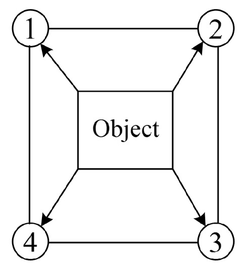
Figure 2. Communication topology.

The length and width of the drilling platform are 110m and 84m [25], respectively. The model parameters of the platform are given as follows:

$$M_0=\left[\begin{array}{ccc}2.16\times {10}^8& 0& 0\\ 0& 4.14\times {10}^8& 2.03\times {10}^8\\ 0& 2.03\times {10}^8& 1.24\times {10}^{11}\end{array}\right]$$

and

$$D_0=\left[\begin{array}{ccc}7.78\times {10}^6& 0& 0\\ 0& 7.9\times {10}^6& 1.54\times {10}^7\\ 0& 1.54\times {10}^7& 1.55\times {10}^{10}\end{array}\right].$$

Th environmental disturbances ${\tau }_d^k$, $k=0,1,\dots ,4$ is modeled as ${\tau }_d^k=R_k^T{b}_k$ [26], where $b\in {\mathbb{R}}^3$ denotes the total disturbances on earth-fixed frame that can described the first Markov process as ${\dot{b}}_k=T_b^{-1}{b}_k+E_k{\omega }_k$, $T_b\in {\mathbb{R}}^{3\times 3}$ denotes the bias time constant matrix, $E_k$ is a diagonal matrix scaling the amplitude ${\omega }_k$, and ${\omega }_k$ denotes the vector of zero-mean Gaussian white noise. In the simulation, the parameters of the disturbances are chosen $T_b={10}^3{I}_3$, $b_0\left(0\right)=[{10}^6\mathrm{kN},{10}^6\mathrm{kN},{10}^8\mathrm{kN}·\mathrm{m}]$, $E_0=\mathrm{diag}\left\{{10}^5,{10}^5,{10}^7\right\}$, $b_i\left(0\right)$$=[{10}^5\mathrm{kN},{10}^5\mathrm{kN},{10}^7\mathrm{kN}·\mathrm{m}]$, $E_i=\mathrm{diag}\left\{{10}^4,{10}^4,{10}^6\right\}$. The towline properties are shown in Table 1. We choose the force when the towline is not stretched as the minimum force. Using the towline model, the minimum force can be calculated, which is equal to 70 kN.

Table 1. Properties of towlines [15].

Length	Diameter	Reference Quality	Axial Rigidity $\mathbf{EA}$	Maximum Force
250 $\mathrm{m}$	54.6$\mathrm{mm}$	12$\mathrm{kg}/\mathrm{m}$	$9.2\times {10}^8\mathrm{N}$	$1\times {10}^7$ N

The angles ${\theta }_i$ of four towlines are set as ${330}^{\circ }$, ${30}^{\circ }$, ${150}^{\circ }$ and ${210}^{\circ }$, respectively. The moment arms $(l_{xi},l_{yi})$ of the floating object are selected as $(55\mathrm{m},-42\mathrm{m})$, $(55\mathrm{m},42\mathrm{m})$, $(-55\mathrm{m},42\mathrm{m})$ and (−55 m, −42 m), respectively. The angles ${\varphi }_i$ are chosen as ${\varphi }_1={\varphi }_3={150}^{\circ }$ and ${\varphi }_2={\varphi }_4={210}^{\circ }$.

The set point is ${\eta }_p={[150 \mathrm{m},150 \mathrm{m},{45}^{\circ }]}^T$. Let ${\eta }_p$ pass through a third-order reference model to generate the desired reference signals ${\eta }_d$, ${\dot{\eta }}_d$ and ${\ddot{\eta }}_d$ [16]. In this simulation, the natural frequency is selected as $0.005\mathrm{rad}/\mathrm{s}$ and damping is selected as 0.9. The initial positions of the floating object and four vessels are provided in Table 2. The initial velocities of the floating object and four vessels are set as zero. The initial estimation of the floating object and four vessels are chosen as ${\widehat{\eta }}_k={\eta }_k$, $k=0,1,\dots ,4$.

Table 2. Initial positions of the floating object and four vessels.

${\mathit{\eta }}_{\mathit{i}}$	${\mathit{x}}_{\mathit{i}}$ (m)	${\mathit{y}}_{\mathit{i}}$ (m)	${\mathit{\psi }}_{\mathit{i}}{(}^{\circ })$
${\eta }_0$	0	0	0
${\eta }_1$	217.5	−167	0
${\eta }_2$	217.5	167	0
${\eta }_3$	−217.5	167	180
${\eta }_4$	−217.5	−167	180

The parameters of the proposed NESOs are chosen as ${\omega }_k=0.8$, $k=0,1,$…$,4$. The control parameters of the platform are chosen as $K_{01}=1.3I_3$ and $K_{02}=0.2I_3$. The control parameters of four vessels are given as $K_{i1}=1.1I_3$ and $K_{i2}=0.15I_3$.

4.1. Simulation of Propsoed Control

The simulation results are shown from Figure 3, Figure 4, Figure 5, Figure 6, Figure 7, Figure 8, Figure 9 and Figure 10. Figure 3 shows the tracking trajectories of the platform and four vessels using the proposed control method under model uncertainties and environmental disturbances, in which one can see that the object can track the reference signal and four vessels are able to track the object with time-varying formation. Figure 4 depicts the tracking error of the floating object under proposed control scheme. It can be seen from the figure that the tracking error of floating body almost converges to zero. Figure 5 shows that four vessels can maintain the desired formation tracking the platform. The tracking errors of four vessels changes in the x and y directions are caused by the heading changes of the floating object.

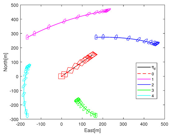
Figure 3. Trajectories of the platform and four vessels using proposed control method.

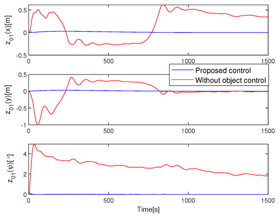
Figure 4. Tracking errors of the platform using two control methods.

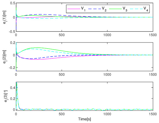
Figure 5. Tracking errors of four vessels using proposed control method. ($V_i$(i = 1,…,4) denotes the ith vessel).

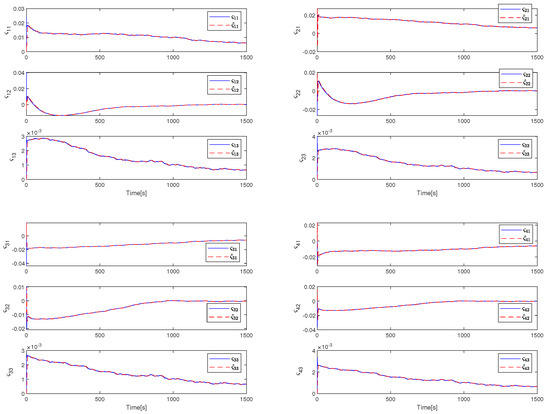
Figure 6. Lumped disturbances and estimations of four vessels.

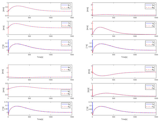
Figure 7. Velocities and estimations of four vessels.

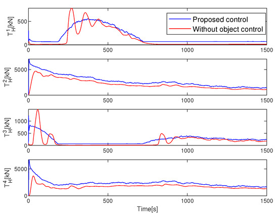
Figure 8. Horizontal tensions along four towlines using two control methods.

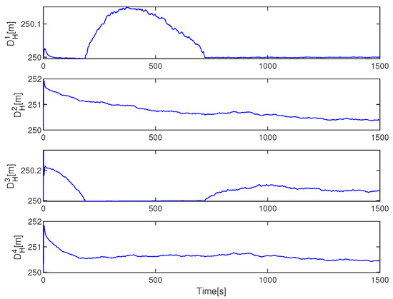
Figure 9. Horizontal distances of four towlines using proposed control method.

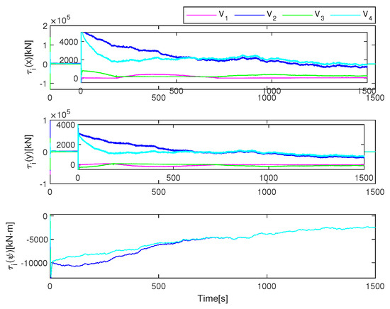
Figure 10. Control inputs of four vessels using proposed control method. ($V_i$(i = 1,…,4) denotes the ith vessel).

Figure 6 shows that the lumped disturbances consisting of model uncertainties and environmental disturbances can be estimated by the proposed NESO. Figure 7 depicts the velocities and estimations of four vessels. It is shown that the velocities can be reconstructed by the proposed NESO. Figure 8 shows the horizontal tensions along four towlines. Figure 9 has closed link to Figure 8, since the horizontal tensions respect the horizontal distances towlines. Figure 10 illustrates that control forces and moments of four vessels are smooth and bounded. As shown in the figure, moments of four vessels eventually converge. However, since four vessels need to provide forces in the x and y directions to maintain the position of the floating object, the control forces in these two directions are not converge in the end.

4.2. Comparison and Analysis

To provide a comparison for the performance of the proposed control method, a distributed output feedback control law without the floating object controller is used to replace the method in [3], which is given as

$$\left\{\begin{array}{cc}\hfill {\vartheta }_i=& {\eta }_{tow}^{di}-{\eta }_d+L_R{B}_d^i\hfill \\ \hfill z_{i1}=& \sum _{j=1}^4{a}_{ij}({\eta }_i-{\eta }_j-{\vartheta }_{ij})+a_{i0}({\eta }_i-{\eta }_d-{\vartheta }_i)\hfill \\ \hfill {\alpha }_i=& \frac{R_i^T}{a_{id}}\left\{-K_{i1}{z}_{i1}+\sum _{j=1}^4{a}_{ij}(R_j{\widehat{\upsilon }}_j+{\dot{\vartheta }}_{ij})+a_{i0}({\dot{\eta }}_d+{\dot{\vartheta }}_i)\right\},\hfill \\ \hfill z_{i2}=& {\widehat{\upsilon }}_i-{\overline{\alpha }}_i\hfill \\ \hfill {\tau }_i=& M_i\left(-K_{i2}{z}_{i2}+{\dot{\alpha }}_i-{\widehat{\varsigma }}_i-a_{id}{R}_i^T{z}_{i1}\right)-{\phi }_i\hfill \end{array}\right.$$

(32)

where $B_d^i={\left[cos({\theta }_i+{\psi }_d),sin({\theta }_i+{\psi }_d),{\delta }_i/L_R\right]}^T$; ${\eta }_{tow}^{di}$ is the desired position of the ith towed point on the floating object, and ${\eta }_{tow}^{di}\left(3\right)={\eta }_d\left(3\right)$; $L_R=250$. The control parameters of (32) are the same as the proposed control method.

The simulation results are shown in Figure 4 and Figure 8. Figure 4 illustrates the tracking performance of the platform using two control methods. It can be seen that the tracking error of the platform under the proposed method is much smaller than the method without the floating object controller in the whole tracking process. This happens because the floating object tracking controller design guarantee the tracking performance of the platform. Figure 8 demonstrates the horizontal tensions on the four towlines using two control methods. It can be seen that the tensions on four towlines using proposed control are smoother than the method without object control. This means that the forces provided by the four vessels is also smoother. Therefore, the proposed control method is more effective for cooperative DP operation for the floating object.

5. Conclusions

This paper focuses on the cooperative DP for an unactuated floating object using multiple vessels under model uncertainties and disturbances only using position-heading information. The floating object is connected to multiple vessels through towlines. The NESOs are developed for the floating object and vessels to reconstruct the unmeasured velocity as well as estimate model uncertainties and disturbances. Observer-based controllers are designed for the floating object and multiple vessels to drive the object to track the references signal and achieve the cooperative control of multiple vessels, respectively. Especially, according to the required force of the object, the desired time-varying formation of vessels is determined by using the towline attachment geometry of the object, control allocation and the towline model. A simulation using four vessels and a drilling platform shows that the proposed control method can drive the platform track the reference signal and time-varying formation of four vessels is also maintained. For future work, it is rewarding to investigate cooperative DP control of unactuated object with the collision-free marine operations and input constraints.

Appendix A.1.

Proof of Lemma 1. 

Choose the following Lyapunov function

$$V_{ko}={\chi }_k^T{P}_k{\chi }_k,$$

(A1)

Taking the time derivative of (A1) along (14), yields

$$\begin{array}{cc}\hfill {\dot{V}}_{ko}=& {\chi }_k^T\left[A_{k0}^T{P}_k+P_k{A}_{k0}+r_k(S_T^T{P}_k+P_k{S}_T)\right]{\chi }_k+2{\chi }_k^T{P}_k{B}_k{\dot{\varsigma }}_k.\hfill \end{array}$$

(A2)

Using Assumption 3 and Young’s inequality, the following inequality holds

$${\chi }_k^T{P}_k{B}_k{\dot{\varsigma }}_k\le \frac{1}{2}{\chi }_k^T{P}_k{B}_k{B}_k^T{P}_k{\chi }_k+\frac{1}{2}{q_k}^2$$

(A3)

If the Equation (15) holds, the Equation (A2) becomes

$$\begin{array}{cc}\hfill {\dot{V}}_{ko}\le & -\underline{\lambda }\left(Q_k\right){∥{\chi }_k∥}^2+{q_k}^2\hfill \\ \hfill \le & -c_{k1}{V}_{ko}+c_{k2}\hfill \end{array}$$

(A4)

where $c_{k1}=\frac{\underline{\lambda }\left(Q_k\right)}{\overline{\lambda }\left(Q_k\right)}>0$ and $c_{k2}={q_k}^2>0$. Then, the state ${\chi }_k$ is bounded. Using $s_k={\Xi }_k^T{\chi }_k$, it can conclude that estimation errors vector $s_k$ is bounded.

□

Appendix A.2.

Proof of Lemma 1. 

Select the Lyapunov function as

$$V=\sum _{k=0}^4{V}_{ko}+\frac{1}{2}{z}_{01}^T{z}_{01}+\frac{1}{2}{z}_{02}^T{z}_{02}+\sum _{i=1}^4\left\{\frac{1}{2}{z}_{i1}^T{z}_{i1}+\frac{1}{2}{z}_{i2}^T{z}_{i2}\right\}.$$

(A5)

Using (19) and (29), the derivation of (A5) is

$$\begin{array}{cc}\hfill \dot{V}=& \sum _{k=0}^4{\dot{V}}_{ko}+z_{01}^T\left[-K_{01}{z}_{01}+R_0\left(-{\tilde{\upsilon }}_0-z_{02}\right)\right]+z_{02}^T\left(-K_{0o2}{R}_0^T{\tilde{\eta }}_0-K_{02}{z}_{02}-R_0^T{z}_{01}\right)\hfill \\ \hfill & +\sum _{i=1}^4\left\{z_{i1}^T\left[-K_{i1}{z}_{i1}+a_{id}{R}_i\left(-{\tilde{\upsilon }}_i+z_{i2}\right)\right.\right.+\sum _{j=1}^4{a}_{ij}{R}_j{\tilde{\upsilon }}_j+\left.a_{i0}{R}_0{\tilde{\upsilon }}_0\right]\hfill \\ \hfill & \left.+z_{i2}^T\left(-K_{i2}{z}_{i2}-K_{io2}{R}_i^T{\tilde{\eta }}_i-a_{id}{R}_i^T{z}_{i1}\right)\right\}.\hfill \end{array}.$$

(A6)

Using Young’s inequality, the following inequalities are hold for any positive constants ${\sigma }_{01}$, ${\sigma }_{02}$, ${\sigma }_{i1}$, ${\sigma }_{i2}$, ${\sigma }_{i3}$, and ${\sigma }_{i4}$.

$$\begin{array}{cc}\hfill -z_{01}^T{R}_0{\tilde{\upsilon }}_0& \le \frac{{\sigma }_{01}}{2}{z}_{01}^T{z}_{01}+\frac{1}{2{\sigma }_{01}}{\tilde{\upsilon }}_0^T{\tilde{\upsilon }}_0\hfill \end{array}$$

(A7)

$$\begin{array}{cc}\hfill -z_{i1}^T{R}_i{\tilde{\upsilon }}_i& \le \frac{{\sigma }_{i1}}{2}{z}_{i1}^T{z}_{i1}+\frac{1}{2{\sigma }_{i1}}{\tilde{\upsilon }}_i^T{\tilde{\upsilon }}_i\hfill \end{array}$$

(A8)

$$\begin{array}{cc}\hfill -z_{02}^T{K}_{0o2}{R}_0^T{\tilde{\eta }}_0& \le \frac{3{\omega }_0^2{\sigma }_{02}}{2}{z}_{02}^T{z}_{02}+\frac{3{\omega }_0^2}{2{\sigma }_{02}}{\tilde{\eta }}_0^T{\tilde{\eta }}_0\hfill \end{array}$$

(A9)

$$\begin{array}{cc}\hfill -z_{i2}^T{K}_{io2}{R}_i^T{\tilde{\eta }}_i& \le \frac{3{\omega }_i^2{\sigma }_{i2}}{2}{z}_{i2}^T{z}_{i2}+\frac{3{\omega }_i^2}{2{\sigma }_{i2}}{\tilde{\eta }}_i^T{\tilde{\eta }}_i\hfill \end{array}$$

(A10)

$$\begin{array}{cc}\hfill z_{i1}^T{R}_0{\tilde{\upsilon }}_0& \le \frac{{\sigma }_{i3}}{2}{z}_{i1}^T{z}_{i1}+\frac{1}{2{\sigma }_{i3}}{\tilde{\upsilon }}_0^T{\tilde{\upsilon }}_0\hfill \end{array}$$

(A11)

$$\begin{array}{cc}\hfill z_{i1}^T{R}_j{\tilde{\upsilon }}_j& \le \frac{{\sigma }_{i4}}{2}{z}_{i1}^T{z}_{i1}+\frac{1}{2{\sigma }_{i4}}{\tilde{\upsilon }}_j^T{\tilde{\upsilon }}_j\hfill \end{array}$$

(A12)

Then, the equality (A6) becomes

$$\begin{array}{cc}\hfill \dot{V}\le & \sum _{k=0}^4{\dot{V}}_{ko}-\left(\underline{\lambda }\left(K_{01}\right)-\frac{{\sigma }_{01}}{2}\right)z_{01}^T{z}_{01}-\left(\underline{\lambda }\left(K_{02}\right)-\frac{3{\omega }_0^2{\sigma }_{02}}{2}\right)z_{02}^T{z}_{02}\hfill \\ & +\sum _{i=1}^4\left\{-\left(\underline{\lambda }\left(K_{i1}\right)-\frac{a_{id}{\sigma }_{i1}+a_{i0}{\sigma }_{i3}+d_i{\sigma }_{i4}}{2}\right)z_{i1}^T{z}_{i1}-\left(\underline{\lambda }\left(K_{i2}\right)-\frac{3{\omega }_i^2{\sigma }_{i2}}{2}\right)z_{i2}^T{z}_{i2}\right\}\hfill \\ & +\left(\frac{1}{2{\sigma }_{01}}+\sum _{i=1}^4\frac{a_{i0}}{2{\sigma }_{i3}}\right){\tilde{\upsilon }}_0^T{\tilde{\upsilon }}_0+\frac{3{\omega }_0^2}{2{\sigma }_{02}}{\tilde{\eta }}_0^T{\tilde{\eta }}_0+\sum _{i=1}^4\left\{\left(\frac{a_{id}}{2{\sigma }_{i1}}+\frac{d_i}{2{\sigma }_{i4}}\right){\tilde{\upsilon }}_i^T{\tilde{\upsilon }}_i+\frac{3{\omega }_i^2}{2{\sigma }_{i2}}{\tilde{\eta }}_i^T{\tilde{\eta }}_i\right\}.\hfill \end{array}$$

(A13)

where $d_i={\displaystyle \sum _{k=1}^4}{a}_{ij}$. Define $l_{01}=\underline{\lambda }\left(K_{01}\right)-\frac{{\sigma }_{01}}{2}$, $l_{02}=\underline{\lambda }\left(K_{02}\right)-\frac{3{\omega }_0^2{\sigma }_{02}}{2}$, $l_{i1}=\underline{\lambda }\left(K_{i1}\right)-\frac{a_{id}{\sigma }_{i1}+a_{i0}{\sigma }_{i3}+d_i{\sigma }_{i4}}{2}$, and $l_{i2}=\underline{\lambda }\left(K_{i2}\right)-\frac{3{\omega }_i^2{\sigma }_{i2}}{2}$. Using ${\chi }_k={\Xi }_k{s}_k$, leads to

$$\begin{array}{cc}\hfill \dot{V}\le & \sum _{k=0}^4{\dot{V}}_{ko}-l_{01}{z}_{01}^T{z}_{01}-l_{02}{z}_{02}^T{z}_{02}+\sum _{i=1}^4\left\{-l_{i1}{z}_{i1}^T{z}_{i1}-l_{i2}{z}_{i2}^T{z}_{i2}\right\}+c_{03}{\chi }_0^T{\chi }_0+\sum _{i=1}^4{c}_{i3}{\chi }_i^T{\chi }_i,\hfill \end{array}$$

(A14)

where

$$c_{03}=max\left\{\frac{3{\omega }_0^2}{2{\sigma }_{02}},\frac{1}{2{\sigma }_{01}}+\sum _{i=1}^4\frac{a_{i0}}{2{\sigma }_{i3}}\right\}$$

(A15)

$$c_{i3}=max\left\{\frac{3{\omega }_i^2}{2{\sigma }_{i2}},\frac{a_{id}}{2{\sigma }_{i1}}+\frac{d_i}{2{\sigma }_{i4}}\right\}.$$

(A16)

Substituting (A4) into (33), yields

$$\begin{array}{cc}\hfill \dot{V}\le & \sum _{k=0}^4-\left\{\left(c_{k1}-\frac{c_{k3}}{\underline{\lambda }\left(P_k\right)}\right)V_{ko}\right\}-l_{01}{z}_{01}^T{z}_{01}-l_{02}{z}_{02}^T{z}_{02}+\sum _{i=1}^4\left\{-l_{i1}{z}_{i1}^T{z}_{i1}-l_{i2}{z}_{i2}^T{z}_{i2}\right\}\hfill \\ & +\sum _{k=0}^4{c}_{k2}\hfill \\ \hfill \le & -{\beta }_{1}V+{\beta }_2,\hfill \end{array}$$

(A17)

where $k=0,1,\dots ,4$, ${\beta }_1=min\{c_{k1}-\frac{c_{k3}}{\underline{\lambda }\left(P_k\right)},2l_{01},2l_{02},2l_{i1},$$\left.2l_{i2}\right\}$, and ${\beta }_2={\displaystyle \sum _{k=0}^4}{c}_{k2}$ is bounded. If the parameters are chosen such that ${\beta }_1>0$, then the Lyapunov function (A5) is bounded. From (A5), it can conclude that all signals in the closed loop system are uniformly ultimately bounded.

Finally, it will show the vessels can track the floating object, and the tracking errors is bounded. Define the tracking error of each vessel as $e_i={\eta }_i-{\vartheta }_i-{\eta }_0$. Letting $z_1={\left[z_{11}^T,\dots ,z_{41}^T\right]}^T$ and $e={\left[e_1^T,\dots ,e_4^T\right]}^T$, it has $z_1=\left(\mathcal{H}\otimes I_3\right)e$, where $\mathcal{H}$ is defined in Section 2. Using Assumption 1, $\mathcal{H}$ is nonsingular. It can obtain that $∥e∥\le \frac{∥z_1∥}{\underline{o}\left(\mathcal{H}\right)}$, where $\underline{o}\left(\mathcal{H}\right)$ is minimal singular value of $\mathcal{H}$. Then $∥e∥$ is ultimately bounded. □

References

- Vu, M.T.; Choi, H.-S.; Kang, J.; Ji, D.-H.; Jeong, S.-K. A study on hovering motion of the underwater vehicle with umbilical cable. Ocean Eng. 2017, 135, 137–157. [Google Scholar]
- Vu, M.T.; Van, M.; Bui, D.H.P.B.; Do, Q.T.; Huynh, T.-T.; Lee, S.D.; Choi, H.-S. Study on Dynamic Behavior of Unmanned Surface Vehicle-Linked Unmanned Underwater Vehicle System for Underwater Exploration. Sensors 2020, 20, 1329. [Google Scholar] [CrossRef]
- Ianagui, A.S.S.; Tannuri, E.A. Automatic load maneuvering and hold-back with multiple coordinated dp vessels. Ocean Eng. 2019, 178, 357–374. [Google Scholar] [CrossRef]
- Chen, L.; Hopman, H.; Negenborn, R.R. Distributed model predictive control for cooperative floating object transport with multi-vessel systems. Ocean Eng. 2019, 191, 1–16. [Google Scholar] [CrossRef]
- Peng, Z.; Wang, D.; Wang, J. Cooperative dynamic positioning of multiple marine offshore vessels: A modular design. IEEE/ASME Trans. Mechatron. 2016, 21, 1210–1221. [Google Scholar] [CrossRef]
- Xia, G.; Sun, C.; Zhao, B.; Xue, J. Cooperative Control of Multiple Dynamic Positioning Vessels with Input Saturation Based on Finite-time Disturbance Observer. Int. J. Control Autom. Syst. 2019, 17, 370–379. [Google Scholar] [CrossRef]
- Thanh, H.L.N.N.; Vu, M.T.; Mung, N.X.; Nguyen, N.P.; Phuong, N.T. Perturbation Observer-Based Robust Control Using a Multiple Sliding Surfaces for Nonlinear Systems with Influences of Matched and Unmatched Uncertainties. Mathematics 2020, 8, 1371. [Google Scholar] [CrossRef]
- Vu, M.T.; Thanh, H.L.N.N.; Huynh, T.T.; Do, Q.T.; Do, T.D.; Hoang, Q.-D.; Le, T.H. Station-Keeping Control of a Hovering Over-Actuated Autonomous Underwater Vehicle Under Ocean Current Effects and Model Uncertainties in Horizontal Plane. IEEE Access 2021, 9, 6855–6867. [Google Scholar] [CrossRef]
- Vu, M.T.; Le, T.H.; Thanh, H.L.N.N.; Huynh, T.T.; Van, M.; Hoang, Q.-D.; Do, T.D. Robust Position Control of an Over-actuated Underwater Vehicle underModel Uncertainties and Ocean Current Effects Using Dynamic SlidingMode Surface and Optimal Allocation Control. Sensors 2021, 21, 747. [Google Scholar] [CrossRef] [PubMed]
- Xia, G.; Shao, X.; Zhao, A. Robust nonlinear observer and observer-backstepping control design for surface ships. Asian J. Control 2015, 17, 1377–1393. [Google Scholar] [CrossRef]
- Værnø, S.A.; Brodtkorb, A.H.; Skjetne, R.; Calabrò, V. Time varying model-based observer for marine surface vessels in dynamic positioning. IEEE Access 2017, 5, 14787–14796. [Google Scholar] [CrossRef]
- Du, J.; Hu, X.; Liu, H.; Chen, C.L.P. Adaptive Robust Output Feedback Control for a Marine Dynamic Positioning System Based on a High-Gain Observer. IEEE Trans. Neural Netw. Learn. Syst. 2015, 26, 2775–2786. [Google Scholar] [CrossRef]
- Li, Y.; Tong, S. Adaptive fuzzy output constrained control design for multi-input multioutput stochastic nonstrict-feedback nonlinear systems. IEEE Trans. Cybern. 2017, 47, 4086–4095. [Google Scholar] [CrossRef] [PubMed]
- Xia, G.; Sun, C.; Zhao, B.; Xia, X.; Sun, X. Neuroadaptive distributed output feedback tracking control for multiple marine surface vessels with input and output constraints. IEEE Access 2019, 7, 123076–123085. [Google Scholar] [CrossRef]
- Tao, J.; Du, L.; Dehmer, M.; Wen, Y.; Xie, G.; Zhou, Q. Path following control for towing system of cylindrical drilling platform in presence of disturbances and uncertainties. ISA Trans. 2019, 95, 185–193. [Google Scholar] [CrossRef] [PubMed]
- Fossen, T.I. Handbook of Marine Craft Hydrodynamics and Motion Control, 1st ed.; John Wiley & Sons Ltd.: Chichester, UK, 2011. [Google Scholar]
- Peng, Z.; Wang, D.; Li, T.; Han, M. Output-Feedback Cooperative Formation Maneuvering of Autonomous Surface Vehicles With Connectivity Preservation and Collision Avoidance. IEEE Trans. Cybern. 2020, 50, 2527–2535. [Google Scholar] [CrossRef]
- Lindegaard, K.P. Acceleration Feedback in Dynamic Positioning. Ph.D. Thesis, Norwegian University of Sicence and Technology, Trondheim, Norway, 2003. [Google Scholar]
- Guo, B.-Z.; Zhao, Z.-L. On convergence of tracking differentiator. Int. J. Control 2011, 84, 693–701. [Google Scholar] [CrossRef]
- Zhao, D.W.; Ding, F.G.; Tan, J.F.; Liu, Y.Q.; Bian, X.Q. Optimal thrust allocation based GA for dynamic positioning ship. In Proceedings of the IEEE International Conference on Mechatronics and Automation, Xi’an, China, 4–7 August 2010; pp. 1254–1258. [Google Scholar]
- Shang, L.B.; Wang, W.; Liu, Z.H. Research on Heuristic Mutated Particle Swarm Optimization Algorithm. In Proceedings of the IEEE International Conference on Unmanned Systems, Beijing, China, 17–19 October 2019; pp. 226–232. [Google Scholar]
- Johansen, T.A.; Fossen, T.I.; Berge, S.P. Constrained nonlinear control allocation with singularity avoidance using sequential quadratic programming. IEEE Trans. Control Syst. Technol. 2004, 1, 211–216. [Google Scholar] [CrossRef]
- Zhao, B.; Xia, G. Recursive-Biased-Generalized-Inverse-based Control Allocation for Dynamic Positioning Vessels with Experimental Results. IEEE Trans. Control Sys. Technol. Under Review.
- Fossen, T.I.; Strand, J.P. Passive nonlinear observer design for ships using Lyapunov methods: Full-scale experiments with a supply vessel. Automatica 1999, 35, 3–16. [Google Scholar] [CrossRef]
- Jin, X.; Tang, W.; Ding, H.; Deng, C. Design of DP controller based on ADRC for semi-submersible platform. Electron. Des. Eng. 2014, 22, 89–91. [Google Scholar]
- Du, J.; Hu, X.; Krstić, M.; Sun, Y. Robust dynamic positioning of ships with disturbances under input saturation. Automatica 2016, 73, 207–214. [Google Scholar] [CrossRef]
Publisher’s Note: MDPI stays neutral with regard to jurisdictional claims in published maps and institutional affiliations. |
© 2021 by the authors. Licensee MDPI, Basel, Switzerland. This article is an open access article distributed under the terms and conditions of the Creative Commons Attribution (CC BY) license (https://creativecommons.org/licenses/by/4.0/).