A Novel Acoustic Sediment Classification Method Based on the K-Mdoids Algorithm Using Multibeam Echosounder Backscatter Intensity

Abstract

The modern discrimination of sediment is based on acoustic intensity (backscatter) information from high-resolution multibeam echo-sounder systems (MBES). The backscattering intensity, varying with the angle of incidence, reveals the characteristics of seabed sediment. In this study, we propose a novel unsupervised acoustic sediment classification method based on the K-medoids algorithm using multibeam backscattering intensity data. In this method, we use the Lurton parameters model, which is the relationship between the backscattering intensity and incidence, to obtain the backscattering angle corresponding curve, and we use the genetic algorithm to fit the curve by the least-squares method. After extracting the four relevant parameters of the model when the ideal fitting effect was achieved, we input the characteristic parameters obtained from the fitting to the K-medoids clustering model. To validate the proposed classification method, we compare it with the self-organizing map (SOM) neural network classification method under the same parameter settings. The results of the experiment show that when the seabed sediment category is less than or equal to 3, the results of the K-medoids algorithm and the SOM neural network are approximately identical. As the sediment category increases, the SOM neural network shows instability, and it is impossible to see the clear boundaries of the seabed sediment, while the K-medoids category is 5 and the seabed sediment classification is correct. After comparing with field in situ seabed sediment sampling along the MBES survey line, the sediment classification method based on K-medoids is consistent with the distribution of the field sediment sampling. The classification accuracies for bedrock, sandy clay, and silty sand are all above 90%; those for gravel and clay are nearly 80%, and the overall accuracy reaches 89.7%.

1. Introduction

Seabed detection and sediment classification have important practical significance for marine engineering construction, seafloor map, biological habitat environment inversion, and seabed resource exploration [1,2,3]. As they are the basis of seabed research, they are important for understanding seabed sediment properties in detail [4]. Traditional seafloor sediment classification usually uses field sediment sampling and discrete field sampling according to a certain grid and confirms the type of sediment after laboratory analysis. Although this method can be used to directly assess the sediment category, it has disadvantages such as high labor intensity, low efficiency, high operating costs, and it is difficult to achieve high-precision surveys in a large area [5]. What is more, the types of sediment between grid nodes are affected by various factors. Nowadays, how to quickly and accurately obtain large-area sediment information is the research focus of oceanographers.

With the development of modern sonar technology, seabed survey equipment such as the multibeam echo-sounder system (MBES), side-scan sonar (SSS), bathymetry light detection airborne ranger (LiDAR), and sub-bottom profiler (SBP) have emerged, which have allowed seabed sediment detection and classification to develop from traditional field sediment sampling to acoustic sediment detection [6,7,8,9]. We can apply acoustic methods to determine the relationship between the acoustic parameters of seabed sediment (such as reflection coefficient, sound velocity, attenuation, and scattering) and the physical properties of the sediment (such as sediment type and particle size distribution), to realize a more accurate classification of sediment [10]. This is an important aspect of the development of acoustic remote sensing in the marine environment [11,12]. Among the seabed survey equipment, SSS can use acoustic imaging to display seabed images [13]. When analyzing seabed topography, it can also be used for research on seabed sediment detection and classification, but it is usually based on the assumption that the seabed is flat [14,15]. LiDAR can directly obtain high-precision three-dimensional coordinates and intensity data on the target surface, but such systems are usually heavy and expensive [16]. An SBP can obtain stratum data, but the coverage is extremely limited [17]. An MBES not only obtains high-precision seabed topographic data but also abundant backscatter intensity data. With the advantages of full coverage, high sampling rate, high efficiency, and low cost, MBES has gradually become an important method for seabed sediment detection and classification [18,19]. Therefore, how to analyze and apply the backscatter strength data of MBES is the focus of seabed sediment classification research [20,21].

The backscatter intensity from the MBES contains explanatory information that is highly correlated with seabed sediment grain size and properties [22,23,24]. However, although backscatter information can roughly portray the characteristics of the seafloor, it is still necessary to establish a relationship model between the backscatter intensity and the type of seabed sediment to achieve the precise classification of the seafloor [25,26,27]. This requires abundant feature extraction, sampling analysis, and statistical analysis [28,29]. Since seafloor backscattering intensity and the categorization of sediment have been proven to have a strong correlation with the angle of incidence, the current relationship between backscattering intensity and sediment characteristics usually needs to be based on the response model between backscattering intensity and the angle of incidence [30].

However, based on the magnitude of the backscatter intensity, we can roughly reflect the sediment information of the seabed, such as whether it is gravel or mud, due to the discreteness of the measured backscattering intensity dataset and the fact that the values of the seabed backscattering intensity for different sediment types may be comparable; there is a one-to-many relationship between the seabed backscattering intensity and sediment type. To eliminate this effect, it is necessary to establish an exact model to reflect the relationship between the type of sediment, the intensity of backscatter, and the angle of incidence [31]. Biot [32,33] proposed a model for the propagation of elastic waves in fluid-saturated porous solids. On this basis, Stoll [34] made an improvement that enabled the calculation of sound velocity and sound attenuation in the seabed sediment medium. According to the natural characteristics of sound scattering at different angles, Jackson [35] divided the seafloor backscattering intensity with the incident angle into three regions and explained the main contribution of the seafloor backscattering intensity in each region. Based on previous research, Hughes [36] processed measured multibeam seabed backscattering intensity data and extracted salient features from the curve of the average backscattering intensity with the angle of incidence to estimate the type of seabed sediment. Landmark and Solberg [37] established a standard Bayesian model through the relationship between angle and backscatter intensity. Santos et al. [38] used the angular distance analysis to analyze the backscattering data obtained by different MBESs, estimated the average particle size of the seabed sediment, and constructed the corresponding relationship between particle size and sediment. Alevizos and Greinert [39] used hyperangular cube data to improve the acoustic resolution of MBES backscatter angular response and used four machine learning algorithms to test the effect of the improved angle response on the sediment classification. After a model of sediment, incidence, and backscattering intensity is established, sediment classification with a certain accuracy can be obtained through the angle response curve.

Theoretically, if there is no deviation in the observed backscattering intensity curve, the extracted characteristic parameters can reflect the diversity of the seabed type. However, in practice, due to the random nature of the backscattering intensity and the shortfalls of data processing, the error for some parameters may be considerable, meaning that they no longer reflect changes in the seabed sediment. If the extracted parameters are still used as the input parameter of the classifier, the classification accuracy will be affected. Lurton et al. [40] established a model of the intensity change of backscattering in the whole angle range based on the natural characteristics of sound scattering at different angles. The model was determined by four parameters. The analysis of the data used by Lurton found that the curve calculated by this model can not only fit the experimental data better but also is not sensitive to limited system deviations.

To make full use of the angular response model to classify seabed sediment, it is necessary to use a more efficient method to evaluate the model parameters. With the continuous development of machine learning, artificial intelligence, big data, and other emerging technologies, MBES sediment classification has realized the transition from traditional statistics to semi-automatic and fully automatic classification, which greatly reduces the workload and subjective deviation of seabed sediment classification. Unsupervised learning and supervised learning are applied to the classification of sediment based on MBES [41,42]. However, supervised learning needs to learn from a training set. Training a classification function or model requires a large amount of seabed sampling data to support seabed sediment classification, which is relatively difficult to achieve. Therefore, unsupervised algorithms have been widely used when the type of sediment is unknown and there is no field sediment sampling. In unsupervised classification, cluster analysis can quickly find the structural information contained in the sample data, so it is widely used in classification. Tegowski [43] used the integral backscattering strength, spectral width, and fractal dimension of the echo envelope as eigenvalues, and performed a K-means analysis to achieve sediment classification in the southern Baltic Sea. However, this method is more sensitive to local value transformation. Marsh and Brown [44] introduced a self-organizing neural network to realize the automatic classification of seabed sediments. Lucieer and Lamarche [45] used a fuzzy C-means (FCM) clustering algorithm to statistically identify sediment samples. Tan et al. [14] proposed a high-order local autocorrelation method to automatically classify the seabed sediment of sonar graphics and verified its classification advantages by comparing it with a traditional gray-level co-occurrence matrix and other texture methods. Chakraborty et al. [46] tested the self-organizing feature map for seabed sediment classification, accurately distinguishing three types of sediment in the research area. These methods have also demonstrated great potential to predict benthic habitats and communities. Since unsupervised sediment classification does not have a training set for learning, there is still a lot of room for development in classification accuracy.

Although the authors of [46] used the self-organizing map (SOM) method to achieve nearly 100% accuracy in the classification of seabed sediment, they used single-beam sonar, which is no longer applicable to current research since multibeam sounding systems are the mainstream. There are only three sediment types in their study area, which makes it questionable whether SOMs are applicable for areas with more sediment types. With the development of machine learning, various clustering methods have been proposed, and the application of more effective clustering methods to classify seabed sediment has become a trend.

In this study, we propose a novel acoustic sediment classification method based on the K-medoids algorithm using multibeam echosounder backscatter intensity. We use Simrad EM3000 MBES backscatter intensity data from China’s Qingdao Jiaozhou Bay to verify the feasibility and accuracy of the proposed seabed sediment classification method. The remainder of this paper is organized as follows. An introduction, including MBES data processing, information on field sampling, and the principles of feature extraction and clustering, is given in Section 2. The experiments, which include parameter extraction results and a clustering analysis, are presented in Section 3 and Section 4. The work is concluded in Section 5.

2. Materials and Methods

In this section, we discuss the experimental data, the principle of the seabed sediment classification algorithm based on the K-medoids algorithm, and the classification principle of the contrast SOM algorithm. In this study, we used 50 ping backscattering intensities as a group and took the average of each group to represent their backscattering intensity. The Lurton model was used to fit the 873 groups of data, and we applied a genetic algorithm [47] to find the best fitting accuracy set of parameter combinations. This parameter combination was used in the K-medoids algorithm for the clustering analysis. To verify the effectiveness of the algorithm, we also used the SOM algorithm with the same parameter combination to perform the same clustering experiment. Below, we briefly introduce the content of these aspects. The experimental process of this research is shown in Figure 1.

2.1. Data

2.1.1. MBES Data

In this study, we acquired the MBES backscatter data in 2002 from Qingdao Jiaozhou Bay, China, using a high-resolution Kongsberg Simrad EM3000 MBES (Kongsberg Maritime AS, Norway), which is a 300 kHz multibeam echosounder system that fans out up to 127 beams at a 130-degree angle, yielding swathes that are up to four times the water depth. It can capture depths in the 1–150 m range at survey speeds of 3–12 knots. More basic specifications are shown in

Table 1. Kongsberg Simrad EM3000 multibeam echo-sounder system (MBES) basic specifications.

Parameter	Settings
operating depth	1–150 m
ping rate	40 Hz
beamwidth	1.5°
across-track coverage	four times the depth
sonar frequency	300 kHz
seafloor detection mode	phase and amplitude bottom detection algorithm
swath width	130°
beams per ping	127
gain	−3 dB

[48,49]. The data area includes the seas off China at 35°57′44″–36°02′49″ N, 120°18′07″–120°21′00″ E, as shown in Figure 2. The water depth of the area is 15–35 m, and the terrain is flat. This Simrad EM3000 MBES is a shallow water multibeam series. Multibeam backscattering intensity data processing mainly includes system error correction and sound intensity compensation correction. In this research, the correction was implemented by Caris HIPS & SIPS 10.4. The system error correction included fixed gain, time-varying gain, sound source level, and beam directivity. The sound intensity compensation correction included propagation loss, seabed incidence, acoustic area, and central beam. The multibeam backscattering intensity data were processed by CMST-GAMB v8.11.02.1 [50]. To more accurately obtain the relationship between the backscattering intensity and the incidence, we used the average value of the backscatter for every 50 pings as a group to represent the angle response curve corresponding to the 50-ping group. Finally, we obtained the corrected average backscatter intensity of −60° to 60° with an interval of 1°.

2.1.2. The Field Sampling Data

A DDC1 type clamshell sampler with a maximum capacity of 0.05 m² is used for field in-situ measurement. The field sampling was carried out every 20 m in the longitudinal direction, every 100 m in the transverse direction in the survey area, with a total of 34,102 points obtained. We selected 873 sampling points that fell on the survey line to research the effect of sediment classification. This study used the Shepard classification system [51] to divide the sediments. Shepard divided a ternary diagram into 10 classes (Figure 3). Each sediment sample is plotted as a point within or along the sides of the diagram, depending on its specific grain size composition. A sample consisting entirely of one component falls at the apex of the diagram. A sediment entirely lacking in one component falls along the side of the triangle opposite that apex. The rest fall somewhere in between. For example, silt contains at least 75% silt-sized particles, “silty sand” and “sandy silt” contain no more than 20% clay-sized particles, and “sand–silt–clay” contains at least 20% of each of the three components. According to Shepard’s diagram, the study area was divided into clay, silty sand, sandy clay, and sand–silt–clay (displayed as the point in Figure 3). The research area also contained gravel and bedrock (Figure 4). In the seabed sediment classification, the higher the similarity of sediment types, the more difficult it is to distinguish them. An analysis of the similarity of the sediment types in the survey area will help us to correctly evaluate the types of seabed sediment. For this study area, the sand–silt–clay was compared with silty sand, in which there is relatively little clay mixed in, and the similarity between the two is extremely high; compared with the clay, sandy clay contains relatively little sand. The impact of this similarity on the classification of seabed sediment will be discussed in the experimental section.

2.2. Lurton Parametric Model

The change in seabed backscattering intensity is a complex function of seabed characteristics, structure, incidence, and frequency. Lurton et al. established a parameter model of backscattering intensity in the entire angle range based on the natural characteristics of sound scattering at different angles:

$$BS\left(\theta \right)=10\log \left[A\exp \left(-\alpha {\theta }^2\right)+B{\cos }^{\beta }\theta \right],$$

(1)

where $BS$ is the seabed backscattering intensity, θ is the seabed incident angle, and A, B, $\alpha$, and $\beta$ are model parameters that have a mathematical instead of practical meaning. This model is derived from the tangent plane model [52], which tends to approximate Kirchhoff near the vertical incidence and obeys the approximate Lambert’s law in other angle regions. For the detailed derivation, see [40].

2.3. Least Squares Fitting

We fitted the characteristic parameters of the Lurton model based on the least-squares method, whose mathematical model is

$$\underset{x}{\min }\frac{1}{2}{\Vert F\left(x,x_{data}\right)-y_{data}\Vert }_2^2=\frac{1}{2}{\displaystyle \sum _{i=1}^n{\left[F(x,x_{dat{a}_i})-y_{dat{a}_i}\right]}^2}$$

(2)

where $x_{data}$ is the given input observation vector, which is the seafloor incidence $\theta$; $y_{data}$ is the observation vector corresponding to $x_{data}$, which is the seafloor backscattering intensity corresponding to the seafloor incidence $\theta$; $F(x,x_{data})$ is the objective function, $BS(\theta )$; x is the fitting coefficient vector of the functions A, B, $\alpha$, and $\beta$; and n is the length of the observation vector which is the modeled parameter.

2.4. Genetic Algorithm

We adopted the genetic algorithm to obtain the minimum error of the least-squares. The genetic algorithm (GA) is a randomized search method that draws on evolutionary laws. It was proposed by Professor Holland in the United States in 1969 [47]. The genetic algorithm starts from an initial population that represents the possible solution to the problem. The population is composed of a certain number of individuals that have been genetically coded. After the initial population is produced, based on the principle of survival of the fittest, better approximate solutions have evolved from one generation to the next. In each generation, individuals are selected according to the fitness of each individual in the problem set, and the genetic operator is used to cross and mutate according to the probability of producing the next generation’s population. This process will cause the offspring population to adapt to the environment better than the previous generation, and the optimal individual in the last generation’s population can be decoded as the optimal solution to the problem. This process is shown in Figure 5.

2.5. K-Medoids

In 1967, MacQueen proposed the K-means algorithm [53]. The basic principle of this algorithm is to assign each sample to the cluster with the nearest center. K-means is an important and successful method in the field of data clustering. The algorithm is an iterative repartitioning strategy: when the algorithm is completed, the dataset is divided into K clusters specified in advance.

However, the K-means algorithm is sensitive to outliers because, when an outlier is assigned to a cluster, it affects the mean of the cluster, causing the mean to deviate from most of the data in the cluster. This makes it difficult to classify based on multibeam data. In contrast, the center point selected by the K-medoids is a point in the current cluster, and the criterion function is the smallest sum of the distances from all other points in the current cluster to the center point, which weakens the influence of outliers on a certain extent [54]. The fundamental strategy of K-medoids clustering is to acquire K clusters in N objects by first indiscriminately finding a typical object (the medoids) for each cluster. Each residual object is clustered with the medoid to which it is the most comparable. The specific algorithm flow is as follows.

Randomly select K points from the overall n sample points as medoids.

According to which is closest to the medoids, assign the remaining N–K points to the class represented by the best medoids.

For all other points in the i-th class except the current medoid point, calculate the value of the criterion function when it is a new medoid, traverse all possibilities, and select the point corresponding to the smallest criterion function as the new medoid.

Repeat the process until the medoids no longer change or the set maximum number of iterations has been reached.

Output the final determined K categories.

2.6. Self-Organizing Feature Map

The self-organizing feature map (SOM) network was proposed by Teuvo Kohonen [55]. The network is self-organizing and self-learning, composed of fully connected neuron arrays.

The SOM network learning algorithm is an unsupervised competitive learning algorithm. It can transform the input pattern of any dimension into a discrete space of lower dimensionality in a topologically ordered manner, which is a feature map: input space H to output space A. Input space H is a set of input vectors, and the dimension of H is equal to that of the input vector; the output space A is a two-dimensional plane in the self-organizing map of a two-dimensional grid. The self-organizing mapping algorithm includes three processes: competition, cooperation, and updating. The process of SOM is shown in Figure 6.

2.6.1. Competition

During the competition, the neuron with the largest output is determined to be the winning neuron. Since the activation function of the neuron is a linear function, the maximum output of a neuron depends on input $u_i$, which is the inner product of the input vector $X={\left[x_1,x_2,\cdots ,x_N\right]}^{\mathrm{T}}$ and weight vector $W_i={\left[w_{i1},w_{i2},\cdots ,w_{iN}\right]}^{\mathrm{T}}\hspace{0.17em}\left(i=1,2,\cdots ,M\right)$.

$$u_i={\displaystyle \sum _{j=1}^N{w}_{ij}{x}_j}$$

(3)

The inner product is equivalent to the minimum Euclidean distance between the input vector and the weight vector when the input vector and the weight vector are both normalized. So, when the input vector is X and the c neuron wins, the condition is satisfied:

$$\Vert X-W_c\Vert =\underset{i}{\min }\Vert X-W_i\Vert ,\hspace{1em}i=1,2,\cdots ,M,$$

(4)

where $\Vert •\Vert$ represents the Euclidean distance between the input vector X and the weight vector W_i.

2.6.2. Cooperation

During the cooperation process, the strengthening center of the winning neuron is determined. The center of the topological neighborhood is the winning neuron obtained from the competition. The neurons in the neighborhood are called excitatory neurons, which are the strengthening center. A simple square neighborhood shape can be used. When the radius of the neighborhood is 0, it can only contain the winning neuron; and when the radius is 1, the neighborhood contains eight neighboring neurons apart from the winning neuron. When the radius increases, the neighborhood enlarges according to this rule. The topological neighborhood is marked as $N_c\left(n\right)$, and it also represents the radius of the topological neighborhood at the nth iteration. Its value changes with the increase in the iterations:

$$N_c\left(n\right)=INT\left[N_c\left(0\right)\left(1-n/N\right)\right],\hspace{0.17em}\hspace{1em}n=0,1,\cdots ,N,$$

(5)

where $N_c\left(0\right)$ represents the initial topological neighborhood radius, N is the total number of iterations, and $INT(•)$ represents the rounding function. It can be seen that the topological neighborhood shrinks continuously as the number of iterations increases.

2.6.3. Update

In the update process, we adopted Hebb learning rules [56] to update the weight vector of neurons in the topological neighborhood of the winning neuron on the grid:

$$W_i\left(n+1\right)=W_i\left(n\right)+\eta \left(n\right)\left[X-W_i\left(n\right)\right]\hspace{0.17em},\hspace{1em}n=0,1,\cdots ,N,$$

(6)

where $\eta \left(n\right)$ is the learning rate, which decreases with the increase in the iterations, and the change rule can adopt Equation (6):

$$\eta \left(n\right)=\eta \left(0\right)\left(1-\frac{n}{N}\right)\hspace{0.17em},\hspace{1em}n=0,1,\cdots ,N,$$

(7)

where N is the total number of iterations and $\eta \left(0\right)$ is the initial learning rate.

3. Experiments

In this section, we discuss the processing flow of the fitting effect of the angle and corresponding curve. Then, when an ideal fitting effect is achieved, the corresponding feature parameters are used as the features of the supervised model for classification. Finally, we compare them with the field sediment sampling to illustrate the effectiveness of the classification.

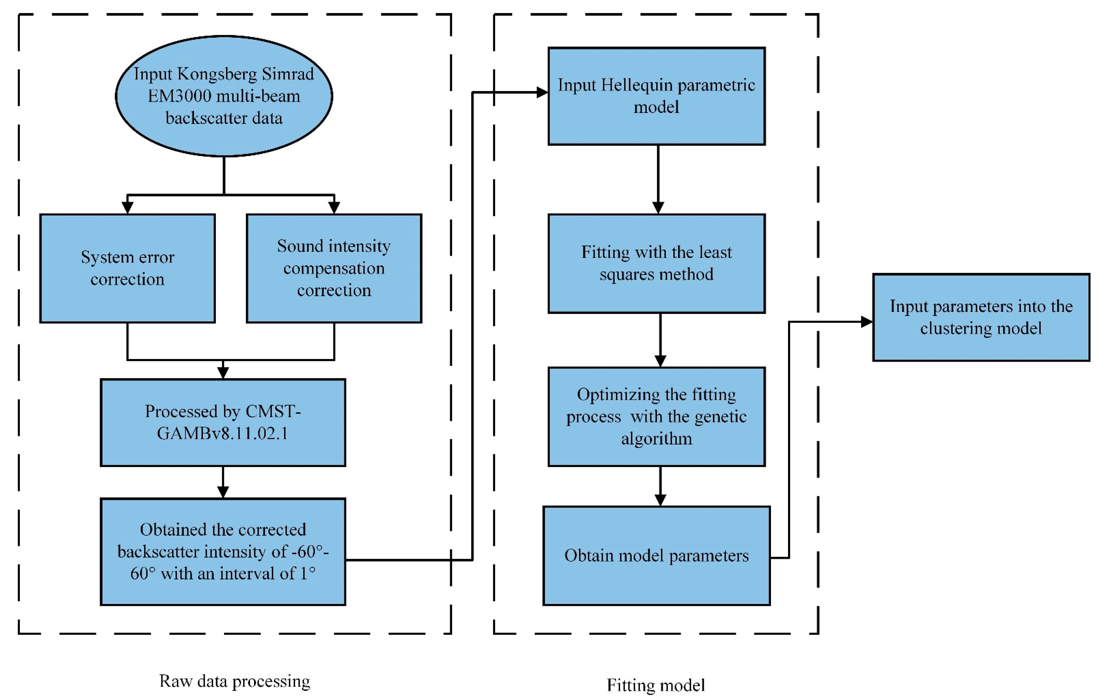
3.1. Fitting Process

To obtain the minimum error, we continuously adjusted the parameters of the genetic algorithm to realize a fitting curve as close to the actual data curve as possible. Finally, the best combination of parameters was determined: Cmax was 500, Generation was 300, Genlength was 10, Popsize was 130, Pcrossover was 0.65, and Pmutation was 0.05. Figure 6 shows the curves of the average backscattering intensity of the bedrock, gravel, clay, sandy clay, silty sand, and sand–silt–clay seabed with the angle of incidence and the fitting curve of the Lurton parameter model.

Figure 7a,b show the bedrock and gravel seabed. It can be seen that the backscattering intensity varies with the angle of incidence. The curves show instability in both the edge beam and the center beam. This is because the bedrock and gravel have a large particle size and the seabed surface is extremely uneven. The inclination of the bedrock or scattered gravel easily causes alterations in the angle of incidence in a small area, and this kind of effect is difficult to remove. Nevertheless, the fitting curve can still reflect the trend of backscattering intensity with the angle of incidence. The silty sand (Figure 7c) and the sand–silt–clay seabed (Figure 7d) have relatively smooth curves of average backscattering intensity with the angle of incidence, and the fitting effect is satisfactory. The fitting curves of the clay seafloor (Figure 7e) and the sandy clay (Figure 7f) are also acceptable. The above analysis shows that the effect of fitting of the curve of the average backscattering intensity with the angle of incidence is related to the size of the seabed sediment granule. If the particle size is small and the curve of the backscattering intensity with the angle of incidence is smooth enough, the parameter model will be better fitted to the actual change curve.

3.2. Fitting Parameters

Due to the influence of residual error, the angular response curves obtained by the different groups of pings are different in the same sediment type area, which will cause a change in the characteristic parameters. If the parameter difference is considerable, it will affect the classification accuracy of the seabed sediment. Therefore, it is necessary to analyze the dispersion and mean changes of characteristic parameters in different seabed sediment regions, and evaluate the ability of characteristic parameters to characterize the sediments.

Since sediment classification is affected by gridding a small number of field samples, the boundary of the sediment area is not accurate. Therefore, we took the field sampling on the average position of every 50 pings along the survey line as the research sample and took them as the type of sediment in the corresponding area... Taking the adjacent 50-ping data as a group, we calculated the average backscattering intensity change curve with the incident angle, obtaining the test sample: bedrock (50 groups), gravel (40 groups), clay (40 groups), sandy clay (40 groups), silty sand (40 groups), and sand–silt–clay (30 groups). The feature parameters were extracted according to Section 2.3 and Section 2.4, and the statistical results were as shown in

Table 2. Statistical of characteristic parameters for inhomogeneous seafloor.

Sediment	Parameter	$10\mathbf{log}\mathit{A}$	$10\mathbf{log}\mathit{B}$	$\mathit{\alpha }$	$\mathit{\beta }$
Bedrock	maximum	−8.3	−14.6	164	1.4
	minimum	−27.8	−21.8	4.2	−2.0
	average	−13.3	24.1	24.1	−0.5
	standard deviation	3.1	1.6	35.1	0.8
Gravel	maximum	−8.0	−17.1	108.2	2.6
	minimum	−17.1	−22.6	9.1	−0.4
	average	−14.0	−18.5	9.8	1.4
	standard deviation	1.9	1.2	30.6	0.7
Clay	maximum	−6.8	−20.4	234.1	2.3
	minimum	−14.9	−17.5	47.8	0.9
	average	−10.2	−19.6	116.2	1.4
	standard deviation	1.8	0.6	27.6	0.3
Sandy clay	maximum	−5.8	−17.2	197.6	1.6
	minimum	−12.8	−20.1	90.1	0.7
	average	−9.6	−18.6	143.2	1.3
	standard deviation	1.9	0.3	24.0	0.2
Silty sand	maximum	−14.7	−24.3	144.9	3.1
	minimum	−18.1	−26.8	107.3	2.2
	average	−16.5	−25.7	114.1	2.8
	standard deviation	0.6	0.4	10.2	0.1
Sand–silt–clay	maximum	−13.8	−23.5	151.8	3.2
	minimum	−18.6	−25.5	104.1	2.3
	average	−16.5	−24.6	116.4	2.9
	standard deviation	0.7	0.5	10.9	0.1

.

Analyzing the statistical results in the table, the standard deviation and extreme values $\beta$ of the characteristic parameters of the bedrock seafloor showed the largest variation range, 2–3 times that of the other sediment characteristics. This shows that the $\beta$ of bedrock has the largest probability of falling into the value range of other sediment feature parameters. It will theoretically reduce the classification accuracy. However, the average of the bedrock seafloor $\beta =-0.5$, which, compared to other sediment types, is a large difference, so although the standard deviation of the bedrock $\beta$ parameter is considerable, due to the large difference in the benchmark, the probability that the bedrock $\beta$ is mixed with other types of sediment is greatly reduced. Therefore, the bedrock seafloor can also have an acceptable sediment classification effect. Parameter $\beta$ is the main parameter that distinguishes the bedrock from other seabed sediment types.

The standard deviation of the characteristic parameters decreases successively in the order of bedrock, gravel, clay, sandy clay, sand–silt–clay, and silty sand. From this, the relationship between the particle size of the seabed sediment and the standard deviation of the characteristic parameters is obtained: the smaller the particle size of the seabed sediment, the smaller the standard deviation of the characteristic parameters, and the closer the model curve is to the actual curve.

The characteristic parameter statistics (extreme values, mean values, standard deviation) of the silty sandy and the sand–silt–clay are indistinguishable, indicating that the characteristic parameters extracted by this method may not be able to distinguish between the two kinds of sediment. Taking into account that the composition of the two is similar, and will not affect the types of sediment in other areas, the two sediments are both planned as silty sand.

3.3. Clustering

3.3.1. Training Step Determination

We set the network competition layer to $S=5$, which means the regional sediment was divided into five categories. Since the number of training steps affects the clustering performance of the SOM network, we set the number of training steps to 10, 100, 500, and 1000. We used a different color to represent the types along the survey line and observed the classification performance (Figure 8). It can be seen when the number of training steps is 500, the type of seabed sediment can be distinguished. As the number of training steps increases, the classification result does not change. Therefore, in the following analysis, the number of training steps of the SOM network was set to 500.

3.3.2. Clustering Experiments

To compare the classification effects and capabilities of the two clustering algorithms, the number of categories $K$ and the network neurons $S$ were set to 2–5, and the results of the sediment classification were as shown in Figure 9 and Figure 10.

4. Results and Discussion

We used different colors to represent the types along the survey line and put the classification results in Figure 9 and Figure 10, we also used 1 to 5 instead of the number of categories and showed the specific experiment results in

Table 3. The classification results of SOM and K-medoids for two to four categories.

Sediment Type	Field Sampling	Number of Categories	K-Medoids Result				SOM Result
Bedrock	206	2	1(206)	2(0)			1(206)	2(0)
		3	1(17)	2(0)	3(189)		1(204)	2(2)	3(0)
		4	1(9)	2(54)	3(0)	4(143)	1(0)	2(15)	3(0)	4(191)
Gravel	44	2	1(44)	2(0)			1(25)	2(19)
		3	1(36)	2(8)	3(0)		1(21)	2(0)	3(23)
		4	1(19)	2(4)	3(6)	4(5)	1(10)	2(18)	3(12)	4(0)
Clay	294	2	1(283)	2(11)			1(262)	2(32)
		3	1(294)	2(0)	3(0)		1(249)	2(0)	3(45)
		4	1(261)	2(33)	3(0)	4(0)	1(85)	2(191)	3(0)	4(18)
Sandy clay	93	2	1(87)	2(6)			1(38)	2(55)
		3	1(90)	2(3)	3(0)		1(10)	2(3)	3(84)
		4	1(80)	2(13	3(0)	4(0)	1(38)	2(15)	3(10)	4(33)
Silty sand	236	2	1(0)	2(236)			1(0)	2(236)
		3	1(0)	2(236)	3(0)		1(0)	2(236)	3(0)
		4	1(0)	2(236)	3(0)	4(0)	1(0)	2(236)	3(0)	4(0)

and

Table 4. A comparison between the classification of K-medoids algorithm and the field sampling data along the survey line when there are five categories.

Sediment Type	Field Sampling	K-Medoids		SOM		K-Medoids Accuracy	SOM Accuracy
Bedrock	206	Bedrock	188	Bedrock	160	91.3%	77.7%
		Gravel	18	Gravel	18
				Sandy clay	25
				Clay	3
Gravel	44	Bedrock	2	Sandy clay	12	75.0%	47.7%
		Clay	9	Clay	11
		Gravel	33	Gravel	21
Clay	294	Sandy clay	25	Sandy clay	143	81.6%	10.9%
		Gravel	29	Gravel	110
		Clay	240	Silty sand	9
				Clay	32
Sandy clay	93	Sandy clay	90	Sandy clay	64	96.8%	68.8%
		Clay	3	Clay	15
				Silty sand	4
				Gravel	10
Silty sand	236	Sandy clay	4	Sandy clay	5	98.3%	97.8%
		Silty sand	232	Silty sand	231
Total	873					89.7%	58.2%

. It can be seen from Figure 9a that when the extracted parameters are automatically divided into two categories ($K=2$) by K-medoids (we used 1 and 2 instead of these two types (Table 3)), silty sand can be distinguished and is consistent with the field sampling, indicating that the silty sand classification result is correct. The SOM network classifies sandy clay and silty sand into the same category. Considering the similarity of the sediment types, clay is the main component of sandy clay, and sand is the main component of silty sand. By comparison, the K-medoids classification groups sandy clay with clay. In addition, as can be seen from Figure 9d, sandy clay is divided into two areas (northwest and southeast); K-medoids classifies the two sandy clay areas into one category, but SOM regards the two areas as having two different types of sediment. Moreover, the classification results of SOM showed a small amount of the second sediment type in the bedrock, clay, and gravel, but the results of the field sampling show that the sediment in these areas are continuous, which proves that the classification of SOM in these areas is inaccuracy. Therefore, when the number of classifications is two, the result of the K-medoids algorithm is more reasonable.

When $K=3$, $S=3$ (Figure 9b,e), we used the symbols 1, 2, and 3 instead of the types divided by the algorithm (Table 3), for the result of K-medoids, except for silty sand, where the bedrock area is divided. Due to the fluidity of tidal water, the bedrock may be covered with gravel or clay, which caused the bedrock range to be smaller than the actual field sampling. However, judging from the regional effects on the map, the classification results are reasonable. From the classification of the SOM network, it can be seen that the sandy clay in the southeast can be correctly distinguished from the silty sand and classified as the same as clay, but the sandy clay area in the northwest is put in the same category as the bedrock. Due to the large difference in particle size between sandy clay and bedrock, it is unreasonable to classify them into one type. Due to the K-medoids algorithm correctly distinguishes sandy clay in these two areas, the classification result of K-medoids is more credible in comparison.

When $K=4$, $S=4$ (Figure 9c,f), we used the symbols 1 to 4 instead of these four types (Table 3). For the result of K-medoids, there was basically no change in the silty sand and bedrock area, but there was a clear distinction between the clay and bedrock transition area. At the same time, the northwest direction (shown in blue on the survey line) shows the first time that the sandy clay and clay were correctly separated. Although the SOM achieved a similar effect when $S=4$, it divided the three areas where clay is the main component into three different categories, which is unreasonable.

When $K=5$ (Figure 10), the sandy clay and clay areas with similar composition are basically classified correctly (Table 4). Although the classification result of the bedrock area is different from the field sampling data and we cannot completely eliminate the influence of the sediment transition area, the overall classification effect is consistent. In the case of $S=5$, the classification of the SOM neural network shows (except for the bedrock and silty sand areas, where there is still a good distinction effect) that the other areas have no obvious boundaries; the classification is chaotic and cannot meet the needs of the sediment investigation.

The above analysis shows that the K-medoids algorithm and the SOM neural network using the feature parameters extracted by the Lurton model can achieve almost the same effect in the classification of seabed sediment when the category number is low, and the identification of the bedrock is always accurate. With the increase in the number of categories, the classification effect of the SOM network is extremely unstable. When $S=5$ the obvious boundary of the seabed sediment cannot be seen except for the bedrock. As the category increases, the K-medoids classification effect gradually stabilizes. When $K=5$ the sediment area is correctly divided. By comparing with the field sampling data, it can be seen that the classification accuracy for the bedrock, sandy clay, and silty sand are all above 90%; the gravel and clay are nearly 80%, and the overall accuracy reaches 89.7% (Table 4).

5. Conclusions and Prospects for Future Research

In this study, we proposed a novel unsupervised acoustic sediment classification method based on the K-medoids algorithm using multibeam backscattering intensity data. Firstly, we used the Lurton parameters model to obtain the backscattering angular response curve, fitted the curve with the least squares, and used the genetic algorithm to solve the optimal value of the least-squares. Secondly, these characteristic parameters were imported into the K-medoids classifiers and SOM network. We analyzed the sediment classification results of the two clustering algorithms through different numbers of categories and obtained accurate classification results by the K-medoids algorithms when there were five categories. Through our experiments, we came to the following conclusions:

(1).

The K-medoids algorithms can be combined with multibeam backscattering intensity for use in seabed sediment classification. The overall classification accuracy in our experiments reached 89.7%, the classification of bedrock, sandy clay, and silty sand were all above 90%, and the gravel and clay were nearly 80%.

(2).

Compared with the SOM clustering algorithm, the K-medoids algorithm has a greater advantage in seabed sediment classification. As the number of categories increases, the classification accuracy continues to improve. When the SOM algorithm can no longer distinguish the obvious sediment boundary, K-medoids is still able to achieve acceptable accuracy.

This shows that the K-medoids algorithm can quickly and effectively identify the type of seabed sediment in China’s Jiaozhou Bay, Qingdao, using multibeam backscatter data. However, the backscattering intensity data were obtained by different multibeam equipment and at different water depths, so there is no definitive classification method suitable for all multibeam equipment and water depths. Therefore, the current multibeam-based sediment classification research still needs field sampling for reference and assistance, so the classification process cannot be truly automated. This requires the quantitative analysis and training of different multibeam sonar data of diverse seabed sediments at different water depths and establishing one or more universal sediment classification models to achieve the automated classification of sediments without field sampling.

In addition, Reference [46] used the SOM algorithm to classify the three types of seabed sediment and obtained close to 100% classification results. In this study, we also used SOM for research and comparison, but the results obtained were not ideal. However, when the sediment category is less than 3, although SOM does not correctly classify similar seabed sediments into one class by particle size, it can still distinguish clear sediment boundaries. We speculate that when there is complex sediment composition, it will interfere with the accuracy of SOM classification. Meanwhile, this phenomenon shows that whether a clustering algorithm is suitable for a specific research area still needs experimental verification. In this study, we used the K-medoids algorithm to obtain a total accuracy of 89.7% when the category is 5. However, it is still unknown whether the K-medoids can achieve similar results in other areas. Therefore, it is hoped that future research can focus on the more effective algorithms to achieve sediment clustering which can be applied in any research region.

References

1. Lanier, A.; Romsos, C.; Goldfinger, C. Seafloor habitat mapping on the Oregon continental margin: A spatially nested GIS approach to mapping scale, mapping methods, and accuracy quantification. Mar. Geod. 2007, 30, 51–76. [Google Scholar] [CrossRef]
2. Menandro, P.S.; Bastos, A.C. Seabed Mapping: A Brief History from Meaningful Words. Geosciences 2020, 10, 273. [Google Scholar] [CrossRef]
3. Pearman, T.R.R.; Robert, K.; Callaway, A.; Hall, R.; Lo Iacono, C.; Huvenne, V.A.I. Improving the predictive capability of benthic species distribution models by incorporating oceanographic data—Towards holistic ecological modelling of a submarine canyon. Prog. Oceanogr. 2020, 184. [Google Scholar] [CrossRef]
4. Schirmer, F. Experimental Determination of Properties of the Scholte Wave in the Bottom of the North Sea. In Proceedings of the Bottom-Interacting Ocean Acoustics: NATO Conference Series 4, La Spezia, Italy, 9–13 June 1980; Kuperman, W.A., Jensen, B., Eds.; pp. 285–298. [Google Scholar]
5. Ellingsen, K.E. Soft-sediment benthic biodiversity on the continental shelf in relation to environmental variability. Mar. Ecol. Prog. 2002, 232, 15–27. [Google Scholar] [CrossRef]
6. Anderson, J.T.; Van Holliday, D.; Kloser, R.; Reid, D.G.; Simard, Y. Acoustic seabed classification: Current practice and future directions. ICES J. Mar. Sci. 2008, 65, 1004–1011. [Google Scholar] [CrossRef]
7. Lincoln, F.; PratsonMargo, H.; Edwards. Introduction to advances in seafloor mapping using sidescan sonar and multibeam bathymetry data. Mar. Geophys. Res. 1996, 18, 601–605. [Google Scholar]
8. De, C.; Chakraborty, B. Model-Based Acoustic Remote Sensing of Seafloor Characteristics. IEEE Trans. Geosci. Remote Sens. 2011, 49, 3868–3877. [Google Scholar] [CrossRef]
9. Brown, C.J.; Smith, S.J.; Lawton, P.; Anderson, J.T. Benthic habitat mapping: A review of progress towards improved understanding of the spatial ecology of the seafloor using acoustic techniques. Estuar. Coast. Shelf Sci. 2011, 92, 502–520. [Google Scholar] [CrossRef]
10. Nafe, J.E.; Drake, C.L. Physical properties of marine sediments. In The Sea; Wiley-Interscience: New York, NY, USA, 1963; pp. 794–814. [Google Scholar]
11. Parrott, D.R.; Dodds, D.J.; King, L.H.; Simpkin, P.G. Measurement and evaluation of the acoustic reflectivity of the sea floor. Can. J. Earth Sci. 1980, 17, 722–737. [Google Scholar] [CrossRef]
12. Jackson, D.R.; Richardson, M. High-Frequency Seafloor Acoustics; Springer Science & Business Media: Berlin/Heidelberg, Germany, 2007. [Google Scholar]
13. Huvenne, V.A.I.; Blondel, P.; Henriet, J.P. Textural analyses of sidescan sonar imagery from two mound provinces in the Porcupine Seabight. Mar. Geol. 2002, 189, 323–341. [Google Scholar] [CrossRef] [Green Version]
14. Tan, Y.; Tan, J.K.; Kim, H.; Ishikawa, S. Automatic Classification of Seabed Sediments Based on HLAC. In Proceedings of the IEEE/SICE International Symposium on System Integration, Kobe, Japan, 15–17 December 2013; pp. 653–658. [Google Scholar]
15. Lucieer, V.L. Object-oriented classification of sidescan sonar data for mapping benthic marine habitats. Int. J. Remote Sens. 2008, 29, 905–921. [Google Scholar] [CrossRef]
16. Wang, C.-K.; Philpot, W.D. Using airborne bathymetric lidar to detect bottom type variation in shallow waters. Remote Sens. Environ. 2007, 106, 123–135. [Google Scholar] [CrossRef]
17. Stevenson, I.R.; McCann, C.; Runciman, P.B. An attenuation-based sediment classification technique using Chirp sub-bottom profiler data and laboratory acoustic analysis. Mar. Geophys. Res. 2002, 23, 277–298. [Google Scholar] [CrossRef]
18. Hughes Clarke, J.; Mayer, L.; Wells, D.E. Shallow-water imaging multibeam sonars: A new tool for investigating seafloor processes in the coastal zone and on the continental shelf. Mar. Geophys. Res. 1996, 18, 607–629. [Google Scholar] [CrossRef]
19. Kenny, A.J.; Cato, I.; Desprez, M.; Fader, G.; Schuettenhelm, R.T.E.; Side, J. An overview of seabed-mapping technologies in the context of marine habitat classification. ICES J. Mar. Sci. 2003, 60, 411–418. [Google Scholar] [CrossRef] [Green Version]
20. Huang, Z.; Siwabessy, J.; Nichol, S.; Anderson, T.; Brooke, B. Predictive mapping of seabed cover types using angular response curves of multibeam backscatter data: Testing different feature analysis approaches. Cont. Shelf Res. 2013, 61–62, 12–22. [Google Scholar] [CrossRef]
21. Brown, C.J.; Blondel, P. The application of underwater acoustics to seabed habitat mapping. Appl. Acoust. 2009, 70, 1241. [Google Scholar] [CrossRef]
22. Chakraborty, B.; Schenke, H.W.; Kodagali, V.; Hagen, R. Seabottom characterization using multibeam echosounder angular backscatter: An application of the composite roughness theory. IEEE Trans. Geosci. Remote Sens. 2000, 38, 2419–2422. [Google Scholar] [CrossRef]
23. De Falco, G.; Tonielli, R.; Di Martino, G.; Innangi, S.; Simeone, S.; Parnum, I.M. Relationships between multibeam backscatter, sediment grain size and Posidonia oceanica seagrass distribution. Cont. Shelf Res. 2010, 30, 1941–1950. [Google Scholar] [CrossRef]
24. Sutherland, T.F.; Galloway, J.; Loschiavo, R.; Levings, C.D.; Hare, R. Calibration techniques and sampling resolution requirements for groundtruthing multibeam acoustic backscatter (EM3000) and QTC VIEW (TM) classification technology. Estuar. Coast. Shelf Sci. 2007, 75, 447–458. [Google Scholar] [CrossRef]
25. Fawcett, J.A.; Fox, W.L.J.; Maguer, A. Modeling of scattering by objects on the seabed. J. Acoust. Soc. Am. 1998, 104, 3296–3304. [Google Scholar] [CrossRef]
26. Holliday, D.V. Theory of sound scattering from the seabed. ICES Coop. Res. Rep. 2007, 286, 7–28. [Google Scholar]
27. Collier, J.S.; Brown, C.J. Correlation of sidescan backscatter with grain size distribution of surficial seabed sediments. Mar. Geol. 2005, 214, 431–449. [Google Scholar] [CrossRef]
28. Preston, J. Automated acoustic seabed classification of multibeam images of Stanton Banks. Appl. Acoust. 2009, 70, 1277–1287. [Google Scholar] [CrossRef]
29. McGonigle, C.; Brown, C.; Quinn, R.; Grabowski, J. Evaluation of image-based multibeam sonar backscatter classification for benthic habitat discrimination and mapping at Stanton Banks, UK. Estuar. Coast. Shelf Sci. 2009, 81, 423–437. [Google Scholar] [CrossRef]
30. Rzhanov, Y.; Fonseca, L.; Mayer, L. Construction of seafloor thematic maps from multibeam acoustic backscatter angular response data. Comput. Geosci. 2012, 41, 181–187. [Google Scholar] [CrossRef]
31. Lamarche, G.; Lurton, X. Recommendations for improved and coherent acquisition and processing of backscatter data from seafloor-mapping sonars. Mar. Geophys. Res. 2018, 39, 5–22. [Google Scholar] [CrossRef] [Green Version]
32. Biot, M.A. Theory of propagation of elastic waves in a fluid-saturated porous solid. I. Low frequency range. II. Higher frequency range. J. Acoust. Soc. Am. 1955, 28, 168–191. [Google Scholar] [CrossRef]
33. Biot, M.A. Theory of propagation of elastic waves in a fluid-saturated porous solid: II. Higher frequency range. J. Acoust. Soc. Am. 1956, 28. [Google Scholar] [CrossRef]
34. Stoll, R.D. Acoustic Waves in Saturated Sediments; Springer: New York, NY, USA, 1974; pp. 19–39. [Google Scholar]
35. Jackson, D.R.; Baird, A.M.; Crisp, J.J.; Thomson, P.A.G. High-frequency bottom backscatter measurements in shallow water. Acoust. Soc. Am. 1986, 80, 1188–1199. [Google Scholar] [CrossRef]
36. Hughes Clarke, J. Toward remote seafloor classification using the angular response of acoustic backscattering: A case study from multiple overlapping GLORIA data. IEEE J. Ocean. Eng. 1994, 19, 112–127. [Google Scholar] [CrossRef]
37. Landmark, K.; Solberg, A.H.S.; Austeng, A.; Hansen, R.E. Bayesian Seabed Classification Using Angle-Dependent Backscatter Data from Multibeam Echo Sounders. IEEE J. Ocean. Eng. 2014, 39, 724–739. [Google Scholar] [CrossRef]
38. Santos, R.; Rodrigues, A.; Quartau, R. Acoustic remote characterization of seabed sediments using the Angular Range Analysis technique: The inlet channel of Tagus River estuary (Portugal). Mar. Geol. 2018, 400, 60–75. [Google Scholar] [CrossRef]
39. Alevizos, E.; Greinert, J. The Hyper-Angular Cube Concept for Improving the Spatial and Acoustic Resolution of MBES Backscatter Angular Response Analysis. Geosciences 2018, 8, 446. [Google Scholar] [CrossRef] [Green Version]
40. Hellequin, L.; Boucher, J.M.; Lurton, X. Processing of high-frequency multibeam echo sounder data for seafloor characterization. IEEE J. Ocean. Eng. 2003, 28, 78–89. [Google Scholar] [CrossRef] [Green Version]
41. Galparsoro, I.; Agrafojo, X.; Roche, M.; Degrendele, K. Comparison of supervised and unsupervised automatic classification methods for sediment types mapping using multibeam echosounder and grab sampling. Ital. J. Geosci. 2015, 134, 41–49. [Google Scholar] [CrossRef] [Green Version]
42. Janowski, L.; Madricardo, F.; Fogarin, S.; Kruss, A.; Molinaroli, E.; Kubowicz-Grajewska, A.; Tegowski, J. Spatial and Temporal Changes of Tidal Inlet Using Object-Based Image Analysis of Multibeam Echosounder Measurements: A Case from the Lagoon of Venice, Italy. Remote Sens. 2020, 12, 2117. [Google Scholar] [CrossRef]
43. Tegowski, J. Acoustical classification of the bottom sediments in the southern Baltic Sea. Quat. Int. 2005, 130, 153–161. [Google Scholar] [CrossRef]
44. Marsh, I.; Brown, C. Neural network classification of multibeam backscatter and bathymetry data from Stanton Bank (Area IV). Appl. Acoust. 2009, 70, 1269–1276. [Google Scholar] [CrossRef]
45. Lucieer, V.; Lamarche, G. Unsupervised fuzzy classification and object-based image analysis of multibeam data to map deep water substrates, Cook Strait, New Zealand. Cont. Shelf Res. 2011, 31, 1236–1247. [Google Scholar] [CrossRef]
46. Chakraborty, B.; Kaustubha, R.; Hegde, A.; Pereira, A. Acoustic seafloor sediment classification using self-organizing feature maps. IEEE Trans. Geosci. Remote Sens. 2001, 39, 2722–2725. [Google Scholar] [CrossRef]
47. Koza, J.R. Genetic Programming: V. 1 On the Programming of Computers by Means of Natural Selection; MIT Press: Cambridge, MA, USA, 1992. [Google Scholar]
48. Rønhovde, L.A. High-resolution beamforming for multibeam echo sounders using raw EM3000 data. In Proceedings of the Oceans ‘99 MTS/IEEE Riding the Crest into the 21st Century Conference and Exhibition, Seattle, WA, USA, 13–16 September 1999. [Google Scholar]
49. Naar, D.F.; Donahue, B.T. High-Resolution Multibeam Survey of ONR Mine Burial and Scour Study Area near Clearwater, Florida. In AGU Fall Meeting Abstracts; American Geophysical Union: Washington, DC, USA, 2002. [Google Scholar]
50. Zhi, H.; Siwabessy, J.; Nichol, S.L.; Brooke, B.P. Predictive mapping of seabed substrata using high-resolution multibeam sonar data: A case study from a shelf with complex geomorphology. Mar. Geol. 2014, 357, 37–52. [Google Scholar] [CrossRef]
51. Shepard, F.P. Nomenclature Based on Sand-silt-clay Ratios. J. Sediment. Res. 1954, 24, 151–158. [Google Scholar]
52. Brekhovskikh, L.M.; Lysanov, Y.P.; Beyer, R.T. Fundamentals of Ocean Acoustics. J. Acoust. Soc. Am. 1998, 90, 566–567. [Google Scholar]
53. Macqueen, J.B. Some methods for classification and analysis of multivariate observations. In Proceedings of the Fifth Berkeley Symposium on Mathematical Statistics and Probability, Berkeley, CA, USA, 21 June–18 July 1965. [Google Scholar]
54. Park, H.S.; Jun, C.H. A simple and fast algorithm for K-medoids clustering—ScienceDirect. Expert Syst. Appl. 2009, 36, 3336–3341. [Google Scholar] [CrossRef]
55. Kohonen, T. The self-organizing map. Proc. IEEE 1990, 78, 1464–1480. [Google Scholar] [CrossRef]
56. Hebb, D.O. The Organization of Behavior; Wiley-Interscience: New York, NY, USA, 1949. [Google Scholar]
Figure 1. Sketch of the experiment process.
Jmse 09 00508 g001
Figure 2. The Jiaozhou Bay area. The red rectangle indicates the trial area and the blue line indicates the survey line.
Jmse 09 00508 g002
Figure 3. Shepard sediment classification system [51].
Jmse 09 00508 g003
Figure 4. Distribution of seabed sediment characteristics.
Jmse 09 00508 g004
Figure 5. Sketch of the genetic algorithm process.
Jmse 09 00508 g005
Figure 6. Sketch of the self-organizing map (SOM) network classification.
Jmse 09 00508 g006
Figure 7. The angular response curves corresponding to different sediment types: (a) bedrock; (b) gravel; (c) clay; (d) sandy clay; (e) silty sand; (f) sand–silt–clay.
Jmse 09 00508 g007
Figure 8. SOM network classification under different training steps.
Jmse 09 00508 g008
Figure 9. The classification results of K-medoids under: (a) two categories; (b) three categories; (c) four categories, and the classification results of SOM under: (d) two categories; (e) three categories; (f) four categories.
Jmse 09 00508 g009
Figure 10. The classification results of SOM and K-medoids for five categories.
Jmse 09 00508 g010