Enhanced Weight-Optimized Recurrent Neural Networks Based on Sine Cosine Algorithm for Wave Height Prediction

Abstract

Constructing offshore and coastal structures with the highest level of stability and lowest cost, as well as the prevention of faulty risk, is the desired plan that stakeholders seek to obtain. The successful construction plans of such projects mostly rely on well-analyzed and modeled metocean data that yield high prediction accuracy for the ocean environmental conditions including waves and wind. Over the past decades, planning and designing coastal projects have been accomplished by traditional static analytic, which requires tremendous efforts and high-cost resources to validate the data and determine the transformation of metocean data conditions. Therefore, the wind plays an essential role in the oceanic atmosphere and contributes to the formation of waves. This paper proposes an enhanced weight-optimized neural network based on Sine Cosine Algorithm (SCA) to accurately predict the wave height. Three neural network models named: Long Short-Term Memory (LSTM), Vanilla Recurrent Neural Network (VRNN), and Gated Recurrent Network (GRU) are enhanced, instead of random weight initialization, SCA generates weight values that are adaptable to the nature of the data and model structure. Besides, a Grid Search (GS) is utilized to automatically find the best models’ configurations. To validate the performance of the proposed models, metocean datasets have been used. The original LSTM, VRNN, and GRU are implemented and used as benchmarking models. The results show that the optimized models outperform the original three benchmarking models in terms of mean squared error (MSE), root mean square error (RMSE), and mean absolute error (MAE).

1. Introduction

In coastal and marine structural engineering, wave height is the main factor that needs to be considered. The wave conditions affect several marine activities and have significant consequences for marine industries. Nevertheless, it is challenging to accurately predict such tasks because the ocean waves are stochastic by nature [1,2]. Thus, estimating the wave heights and their trends was, and still is, a big challenge that has to be tackled [3,4].

At early stages, semi-analytic models, such as the Pierson–Neumann–James and Sverdroup–Munk–Bretscheider models, were used to predict the height of the waves; still, such models are inefficient at clearly describing in detail the wave conditions of the sea surface [5,6]. After that, numerical models have been widely used for wave height prediction; nevertheless, such models require a high computational resource when dealing with large amount of data [7,8].

Metocean data are the combination of meteorology and oceanography parameters that need to be studied in order to predict the oceanic environmental change [9]. The meteorology parameters are wind speed, direction, humidity, and air temperature. The oceanography parameters are wave height, period, current, and tides [10,11]. The prediction of oceanic environmental change is essential when planning coastal and offshore constructions, maintenance, or operation. A high-accuracy prediction of these parameters in the offshore environment reduces cost, time consumed, and fault risk. It also helps in determining the required weather window to achieve the projects in time.

Deep learning models were recently applied to atmospheric observation [12,13]. First, the height of the wave has been predicted based on Artificial Neural Network (ANN) models. For instance, a feedforward network model was utilized to forecast the real-time wave height [14]. Similarly, Mandal et al. [15] proposed a Recurrent Neural Network (RNN) for forecast wave height and showed better correlation coefficient compared to feedforward network. Another study conducted by Mahjoobi et al. [16] predicted wave height based on regressive support vector machine (SVM). Their outcomes demonstrated that the proposed model outperforms ANN model in terms of accuracy and computational time. Likewise, ANNs backpropagation and feedforward were compared against model trees to indicate the superiority of predicating wind speed as well as wave height and found that model trees is superior [17].

The ultimate objective of sea wave prediction modeling is to find precise short- or long-term forecasts of the studied variables at a certain time and location [18,19]. The literature of oceanic modeling characteristic is categorized into physical-based and model-based methods [20,21]. These methods have been utilized to forecast ocean waves. According to the work in [3], which was based on the work in [21], these approaches are further graded based on their attempts to specifically parameterize ocean wave interactions. Physical-based methods mimic sea waves by finding the appropriate equation solutions and have been proven to be beneficial over longer time periods for forecasting, whereas model-based methods can be considered as time-series or statistical methods and work well for short-term prediction [22,23,24,25,26]. Moreover, machine learning (or statistical) models can be applied to postprocess physics-based models [27,28,29,30,31].

The main contribution of this study is to predict the wave height with high accuracy and less computational cost. We precisely investigated the following objectives:

• To propose an enhanced weight-optimized RNN based on SCA optimization to process time-series data with high accuracy.
• Three variants of RNNs are enhanced based on SCA: VRNN-SCA, LSTM-SCA, and GRU-SCA.
• To update and tune the learning rate based on grid search mechanism.
• To compare the proposed models against three well-regarded prediction models: LSTM, GRU, and VRNN, then investigate whether the proposed models outperforms in terms of mean squared error (MSE), root mean square error (RMSE), and mean absolute error (MAE).

The rest of this paper is categorized as follows. Section 2 reviews the recent related work on recurrent neural network models for predictions. Section 3 describes metocean data properties and four stations information in different locations. Section 4 explains the methodology, and Section 5 illustrates the experimental setup. Results and discussion are explained in Section 7. Last, this paper is concluded in Section 8.

2. Related Work

Artificial neural network models are labeled to fill within the model-based category, and several neural networks have been utilized to forecast and reconstruct wave characteristics. Artificial Intelligence (AI) models have become an alternative to numerical models in recent years. These models are relatively simple to assemble and have outperformed computational and statistical models for a site-specific wave parameter [32]. The metocean data can be modeled and featured by applying the feature selection algorithms [20,33,34,35,36,37]. Fully connected neural networks in [38] were used to forecast wave heights. RNNs were used in [32] to predict the waves and showed a better correlation Coefficient forecasting. A fuzzy logic modeling machine was also used in [32] to predict the ocean wave energy. An extreme learning machine was applied in [39].

Several studies have been conducted using meta-heuristic algorithms to improve neural network prediction. For instance, Zhang et al. [40] used a fruit fly optimization algorithm and kernel extreme learning machine for bankruptcy prediction. Zhao et al. [41] improved ant colony optimization by utilizing a chaotic intensification strategy and random spare strategy for multi-threshold image segmentation. Tu et al. [42] proposed an improved whale optimization algorithm to overcome the local optimum stagnation problem as well as slow convergence speed. Similarly, the whale optimizer was improved using chaotic multi-swarm to boost support vector machine for medical diagnosis [43]. Shan et al. [44] proposed an improved moth flame optimizer based on a mechanism of adaptive weight. Besides, an enhanced moth flame optimizer-based Gaussian mutation, Levy mutation, as well as Cauchy mutation was proposed for global optimization [45]. Similarly, chaotic moth flame optimizer was utilized in [46] to boost kernel extreme learning machine for medical diagnoses. Chen et al. [47] proposed a new variant of Harris hawks optimizer by integrating several strategies such as topological multi-population, chaos, as well as differential evolution.

Comparative studies have been carried out in [48], taking into account geographical differences and using different neutral networks. The findings show that networks with less allocation of resources have a better structure and adaptability to different situations and conditions [1]. Wang et al. [7] used an evolutionary hybrid algorithm to simulate the ocean waves. This method demonstrated better results than other neural networks in which fewer weather data were available. A symbiotic organisms hunt in [49] was proposed to forecast ocean wave heights in two time zones based on a large number of accurate weather data including wave heights measured by buoys. The proposed model performed better than other state-of-the-art models. In [50], the efficiency of optimization algorithms in resolving real-world complex problems such as the wave height problem is discussed by proposing hybrid approach based on accent-based multi-objective particle swarm optimization algorithm, whereas in [20], a sequence-to-sequence neural network, feature selection, and bayesian hyperparameter are the techniques that were used and applied to forecast the height of the wave and reconstruct a prediction for neighboring buoys stations.

For time series forecasting, researchers apply cross-validation as a technique to distribute the data as in [51,52]. However, cross-validation approaches can be applied to stationary synthetic time series. Besides, using cross-validation depends mainly on the type of the data. Therefore, in our study we used the Out-of-sample (OOS) method, which is traditionally used to estimate predictive performance in time-dependent data.

Despite the good performance of such models, they still face some limitations. For example, feedforward models do not perform well with big time-series data. The RNNs face the phenomenal issue of vanishing gradient. Recently, Rashid et al. [53] attempted to use a set of meta-heuristics algorithms, such as Harmony search, GWO, as well as SCA, in order to overcome the vanishing gradient in LSTM. Similarly, Somu et al. [54] proposed an improved SCA using a Haar wavelet-based mutation operator to optimize the hyperparameters of LSTM for energy consumption prediction [55]. In this paper, the main contribution is to utilize the SCA to enhance the weight of three different types of RNN: LSTM, VRNN, and GRU to forecast wave heights with high accuracy, so that instead of random weight initialization, SCA generates weight values that are adaptable to the nature of the data and model structure. Furthermore, GS is employed to automatically find the best models’ configurations. Besides, according to the No free Lunch theorem [56], there is no specific model to solve all forecasting problems. As such, improvements can be made to the existing models to enhance the performance of such models [57].

3. Study Area

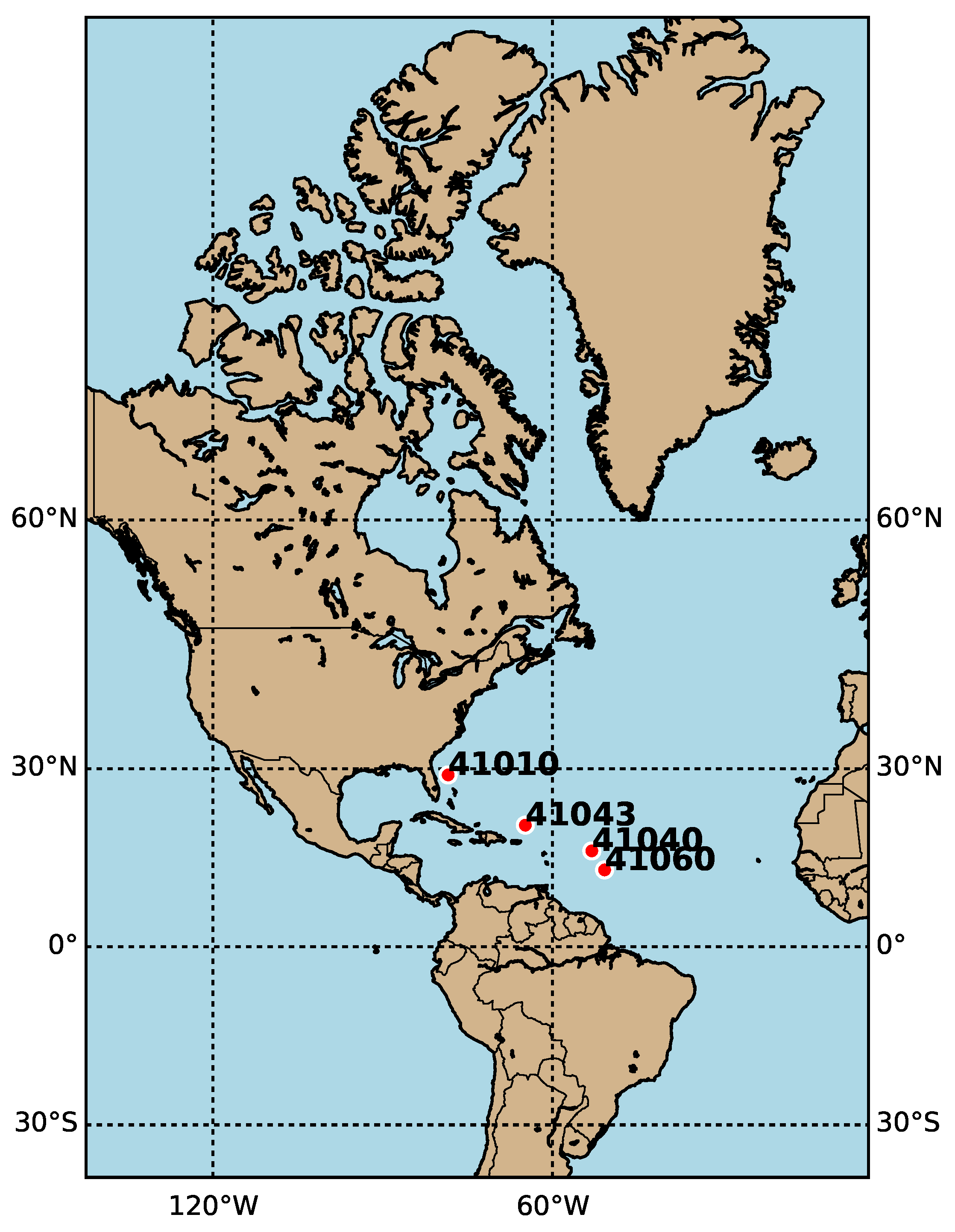
In order to measure the efficiency of the proposed models, four stations were selected from different locations, having several climate conditions as well as variants depths of water. The hourly data that have been used in this study were recorded by floating buoys located in the North Atlantic Ocean.

Table 1. Stations’ dataset.

Station ID	Lon (W)	Lat (N)	Water Depth (M)	SWH (M)	Range Years (Interval)	Training Points	Test Points
41010	28.878	78.485	890	[0.00, 4.6]	[2005,2017]	86356	37011
41040	53.045	14.554	5112	[0.00, 8.09]	[2005, 2017]	54794	18617
41043	64.830	21.124	5271	[0.00, 13.42]	[2007, 2017]	114990	49282
41060	51.017	14.824	5021	[0.72, 4.89]	[2012, 2017]	28952	12409

contains the details of the four stations, and Figure 1 depicts their distribution.

The selected data obtained from the NOAA (https://www.ndbc.noaa.gov/, accessed on 24 December 2020). Four stations are used in this study: Station (41010) (https://www.ndbc.noaa.gov/station_page.php?station=41010, accessed on 24 December 2020); Station (41040) (https://www.ndbc.noaa.gov/station_page.php?station=41040, accessed on 11 January 2021); and Stations (41043) (https://www.ndbc.noaa.gov/station_page.php?station=41043, accessed on 5 January 2021). The details of these stations are described in Table 1. The stations are owned and maintained by National Data Buoy Center National Data Buoy Center, the world’s largest environmental data buoys network [58].

The fourth station (41060) (https://www.ndbc.noaa.gov/station_page.php?station=41060, accessed on 17 Janury 2021) is owned and maintained by Woods Hole Northwest Tropical Atlantic Wave Station (http://uop.whoi.edu/currentprojects/currentprojects.html, accessed on 17 January 2021), which mainly focuses on studying the physical process in ocean surface using moored surface buoys that have metrological and oceanographic sensors.

The wave height is influenced by several factors such as direction and speed of wind, past wave height, and temperature of ocean surface [59,60]. The dataset of each station contains the following features: wind speed, significant wave height, wind direction, gust speed, dominant wave period, the direction from which the waves at the dominant period are coming, average wave period, air temperature, dewpoint temperature, sea surface temperature, sea level pressure, the water level in feet above or below mean lower low water, station visibility, and pressure tendency.

4. Methods

In this section, the main methods used in this paper are explained. First, the original VRNN is outlined, followed by LSTM then GRU. After that, the SCA algorithm is mathematically presented and finally the GS mechanism is elaborated.

4.1. Vanilla Recurrent Neural Network (VRNN)

The simplest structure of VRNN is initialized with one single input layer, one single hidden layer, and one single output layer [61]. Simple architecture is constructed of three layers that can process the sequence of T inputs through time t, which is the vector of $\left\{\dots ,x_{t-1},x_t,x_{t+1},\dots \right\}$. The $x_t=\left\{x_1,x_2,\dots x_T\right\}$, where T is the different length series of the $x_t$ inputs.

All three layers are hierarchically joined from input layer to the hidden layers and from the hidden layer to the output layer. The link between the layers of the network is called a weight matrix. $W_W$ defines the weight connection between the hidden layer and the input layer at each time-step. Equation (1) computes the hidden layer recursively to measure the current state of the network. $W_V$ is the weight matrix reference that links the hidden layer units to each other. The number of hidden units H is $h_t=\left\{h_1,h_2,\dots h_H\right\}$.

$$s_t=W_W{x}_t+W_V{h}_{t-1}+b_h$$

(1)

The $W_W$ matrix is multiplied by the $x_t$ inputs and summed up with the product of $W_V$ and the previous state $h_{t-1}$. Then, this result is added to bias $b_h$ of the hidden layer. Equation (1) defines this process. Equation (2) define the networks’ current state.

$$h_t=f_H\left(s_t\right)$$

(2)

$f_H(.)$ represents the nonlinear activation function that converts the result of $s_t$ to values that depend on the selected activation function. Meanwhile, several activation functions on the state-of-the-art such as sigmoid, tanh, relu, leaky relu, and many more [62,63,64].

$W_U$ is the weight matrix that connects hidden and output layers. The output numbers is N units and can be represented as $y_t=\left\{y_1,y_2,\dots ,y_N\right\}$, while ${\widehat{y}}_t$ is the network prediction that can be obtained by Equation (3).

$${\widehat{y}}_t=f_s(W_U{h}_t+b_o)$$

(3)

The result of the output layer is the sum of product of weights $W_U$ and current hidden state $h_t$ form Equation (2), added to bias of output layer $b_o$, then it is transformed by activation function $f_s(.)$. The output layer predicts the results at each time step based on the results of the hidden layers calculations and input values. ${\widehat{Y}}_t$ defines the total prediction length parameter. The ${\widehat{y}}_t=\left\{{\widehat{y}}_{t1},{\widehat{y}}_{t2},\dots ,{\widehat{y}}_{\widehat{Y}}\right\}$.

4.2. Long Short-Term Memory (LSTM)

LSTM is a new improved variant of RNN that has been proposed to solve the classical version VRNN in terms of gradient problem [65]. Nevertheless, because of different memory cells, LSTM is more expensive in terms of computational resources and requires extra memory compared to RNN [65]. Typical LSTMs have almost four times more parameters than simple VRNN; thus, they suffer from high complexity in hidden layers. The main goal of designing LSTM is to solve the difficulties of learning long-term dependencies, regardless of the uncertainty of their costs [61,66].

The LSTM cell is constructed of several main gates, which are the input gate, forget gate, and the output gate. Irreverent information that has less importance on the prediction is dropped out by the forget gate. By this mechanism, LSTM determines which new data are going to be processed in the cell state [61]. The cell state is altered by the forget gate positioned below the cell state and by the input gate. The previous cell state forgets and adds new information through the output of input gates. The forget gate decides which data should be dropped. It forgets the irrelevant details coming from the previous state with the following calculation in Equation (8) [61,67]. The input gates decide which cell state or long-term memory information can enter. There are two sections to this layer: One is the sigmoid function, while the other is the function of $tanh\left(\right)$. Typically, the target vector is called the “output gate”. The following equations explain the parameter notations in LSTM cell.

$$i_t=\sigma (W_{xi}{x}_t+W_{hi}{h}_{t-1}+W_{ci}{c}_{t-1}+b_i)$$

(4)

$$f_t=\sigma (W_{xf}{x}_t+W_{hf}{h}_{t-1}+W_{cf}{c}_{t-1}+b_f)$$

(5)

$$g_t=tanh(W_{xg}{x}_t+W_{hg}{h}_{t-1}+b_g)$$

(6)

$$o_t=\sigma (W_{xo}{x}_t+W_{ho}{h}_{t-1}+W_{co}{c}_t+b_o)$$

(7)

$$c_t=f_t\otimes c_{t-1}+i_t\otimes g_t$$

(8)

$$h_t=o_t\otimes tanh\left(c_t\right)$$

(9)

$${\widehat{y}}_t=h_t$$

(10)

The $f_{\left(t\right)}$ is the forget gate, $i_{\left(t\right)}$ is the input gate, and $o_{\left(t\right)}$ is the output gate. $g_{\left(t\right)}$ is the method that checks the current input of $x_{\left(t\right)}$. The previous short-term memory is $h_{(t-1)}$. $C_{(t-1)}$ is the previous long-term memory state. The logistic sigmoid function is $\sigma$ and the $tanh\left(\right)$ is the tanh function. ${\widehat{y}}_t$ is the expected prediction output of the LSTM cell. The $c_{\left(t\right)}$ is the long-term state for the next cell, and the $h_{\left(t\right)}$ is the short-term state for the next cell.

$W_{xi}$, $W_{xf}$, $W_{xg}$, and $W_{xo}$ are the connecting weight matrices between the input $x_t$ and the four layers. On the other hand, the connections between the previous state $h_{(t-1)}$ and the four layers are $W_{hi}$, $W_{hf}$, $W_{hg}$, and $W_{ho}$. Every layer has its own bias as $b_i$, $b_f$, $b_g$, and $b_o$, respectively.

4.3. Gated Recurrent Units (GRU)

Cho et al. [68,69] introduced GRU to solve the problem of decay of information that occurs in the traditional recurrent neural network and minimize the computational complexity in LSTM. Two controlling gates are used by GRU, which are the updating and resetting gates that track the data forwarded to the output gate. The update gates decide the past and present data that must be moved to the new state, while the reset gate determines the previous data that must be dropped at every time step. The parameters of the GRU cell are defined by the following equations.

$$Z_t=\sigma (W_{xz}{x}_t+W_{hz}{h}_{t-1}+b_z)$$

(11)

$$R_t=\sigma (W_{xr}{x}_t+W_{hr}{h}_{t-1}+b_r)$$

(12)

$$g_t=tanh(W_{xg}{x}_t+W_{hg}(R_t\otimes h_{t-1})+b_g)$$

(13)

$$h_t=Z_t\otimes h_{t-1}+(1-Z_t\otimes g_t)$$

(14)

where $Z_t$ is the update gate and $W_{xz}$ is the weight matrix between input layer and the update gate, whereas $W_{hz}$ is the weights connecting the update gate with the hidden state $h_{t-1}$. $b_z$ is the bias of the updating gate.

$R_t$ representing the reset gate which is connected to the input layer by $W_{xr}$, while $W_{hr}$ is the weight matrix that connects it to the hidden state $h_{t-1}$. The bias that belongs to this gate is $b_z$.

4.4. Sine Cosine Algorithm (SCA)

SCA is a population-based optimization technique that randomly generates multiple possible solutions for optimization problems. Using the mathematical Sine-Cosine equations to oscillate towards or outwards in order to find the optimal solutions. It uses random variables to adaptively ensure this technique emphasizes on the exploitation and exploration to finding the possible global optima on the search space [70,71]. SCA has been found more efficient than other population-based algorithms in achieving an optimal global solution [54]. Different millstones on the search area are investigated when the sine and cosine functions return values greater than one or less than one. Equations (15) and (16) demonstrate the formation of sine and cosine functions.

$$X_i^{t+1}=X_i^t+r_1*sin\left(r_1\right)*|r_3{P}_i^t-X_i^t|$$

(15)

$$X_i^{t+1}=X_i^t+r_1*cos\left(r_1\right)*|r_3{P}_i^t-X_i^t|$$

(16)

where $X_i^t$ is the position of the current candidate at the tth iteration in the ith dimension AND $P_i$ is the position of the best candidate at the tth iteration in the ith dimension. The random agents are $r_1,r_2,r_3$, and $r_4$. The $(*)$ is the multiplication sign. Equations (15) and (16) are combined in Equation (17).

$$X_i^{t+1}=\left\{\begin{array}{c}{X}_i^t+r_1*sin\left(r_1\right)*|r_3{P}_i^t-X_i^t|,r_4<0.5\hfill \\ X_i^t+r_1*cos\left(r_1\right)*|r_3{P}_i^t-X_i^t|,r_4\ge 0.5\hfill \end{array}\right.$$

(17)

The first agent $\left(r_1\right)$ is responsible for defining the afterward search space, located between the solution region or outside it. The second operator $\left(r_2\right)$ defines the amount of distance in the search space that should be in or out of the destination

$$r_i=a-t\frac{a}{T}$$

(18)

where T indicates the maximum iterations number and t is the currently running iteration. The a is a constant variable. Algorithm 1 shows the main pseudocode of SCA algorithm.

4.5. Grid Search (GS)

In order to produce good accurate results, deep learning models require many parameters that need to be predefined before the training takes place [72,73]. These hyperparameters have to be suitable for the network structure and the nature of the dataset. Setting these hyperparameters can be accomplished manually by trial and error until the best results are achieved; however, this is an inefficient method as it consumes time and may not work as expected [68,74]. Therefore, there are many hyperparameter tuning techniques that have automatically configured models to make them suitable to the network’s structure [75,76].

Grid Search is a hyperparameter tuning technique that can be applied to find the best model configuration [77]; it produces more accurate results [75,78]. Therefore, in this paper, GS has been utilized to obtain the best learning rate values.

Algorithm 1: Algorithm SCA

Input:        • Set the lower bound and upper bound of X solutions       • Set the population size       • Initialize the agents of the search space randomly       • Specify the maximum number of iterations Output:         • The best-selected solution $(X*)$ LOOP Process 1: while$(t\le \mathit{Max}\mathit{number}\mathit{of}\mathit{iterations}T)$do 2:    Calculate every single solutions candidate 3:    Define the best-selected solution $(X*)$ 4:    Update $r_1,r_2,r_3,and{r}_4$ 5:    Update agents’ locations in the search space with (18) 6: end while Return (X*)

5. The Proposed Enhanced Weight Optimized Recurrent Neural Networks

The models developed in this paper have been achieved by integrating the sine cosine algorithm [70] to optimize and update the model weights of simple recurrent neural networks aiming to overcome the problem of vanishing gradient in prediction wave heights. Besides, we integrated an effective grid search mechanism to find the optimal configuration of models’ structures.

The main contribution is to generate weight values that are adaptable to the nature of dataset and models’ structure. To achieve that, instead of initializing the weights of recurrent neural networks randomly, the weight initialization is adapted using SCA algorithm. As explained in the literature, the traditional training of RNNs is usually based on back propagation so that parameters, such as weights and leaning rate, would be updated either by increasing their values or decreasing it until finding the optimal values, resulting in minimizing the error value. The random initialization of the weights was developed to overcome the drawbacks of the back propagation and to enhance the convergence speed with less time. However, the randomness of weight initialization might not be adaptive with every data type and size [79]. Therefore, we proposed an enhanced weight optimized model to effectively overcome the limitations of the state-of-the-art methods, as well as to be more adaptive to any type of dataset.

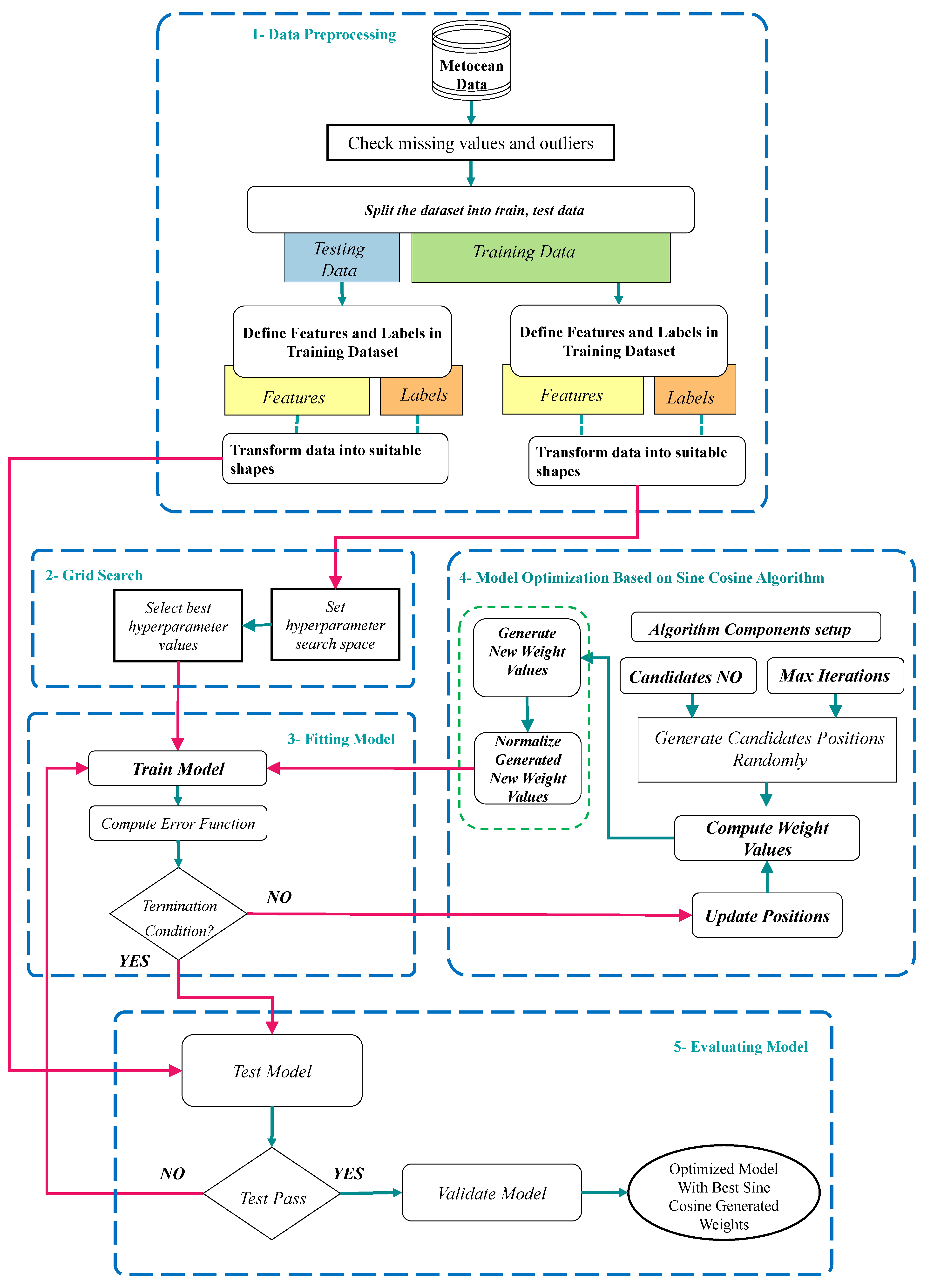
The general structure of the proposed model is illustrated in Figure 2. The following subsections demonstrate the phases of the proposed model to analyze the metocean data and predict the wave heights.

5.1. Data Preprocessing

As explained in Section 3, the four datasets that have been used in this paper were selected from different locations based on Table 1. The datasets have been preprocessed as follows:

• The linear interpolation is used to handle the missing values.
• The time series dataset has been partitioned into 70% for training data and 30% for testing data; 25% of the training portion was assigned for validation.
• After splitting the dataset, the input features and target labels are identified.
• Finally, the MinMaxscaler function from a Python library named Scikit-Learn has been utilized as a normalization technique to scale the data into a suitable form within the range (0, 1).

5.2. Grid Search Mechanism

The optimal hyperparameters are essential in any neural network to obtain sufficient performance. Traditionally, trial and error was used to find the best hyperparameters; however, this technique is not effective as it takes a long time and, in most cases, the optimal values are not guaranteed. It needs to try to set the parameters, train the model, validate, test, and compute the error. This cycling process needs to be repeated many times until it begins getting better results.

Therefore, we integrate an effective technique known as grid search to efficiently find the best hyperparameters for the proposed models.

Table 2. Grid search space parameters.

Grid Search Parameters	Initialization Values
learn_rate	[0.001, 0.01, 0.1, 0.2, 0.3]
dropout_rate	[0.0, 0.1, 0.2, 0.3, 0.4, 0.5, 0.6, 0.7, 0.8, 0.9]
batch_size	[32, 50, 64]
momentum	[0.0, 0.2, 0.4, 0.6, 0.8, 0.9]

shows the parameter settings of the grid search.

Table 2 shows the values of the search space that allows the GS to find and selects the optimal values that are suitable to dataset size and model structure. To avoid the vanishing and exploding gradient problem, the optimal learning rate should not be too small nor too big. Therefore, we set the search space to be between 0.001 and 0.3.

5.3. Weight Optimization Process Using SCA

SCA is a recent effective optimization algorithm capable of exposing an efficient performance and proved to be more effective than several optimization algorithms for attaining optimum or near optimum solution; therefore, it has been selected in this study due to its special characteristics, which are summarized as follows.

• The potential to escape the local optima, besides the high exploration inheritance of sine and cosine functions.
• The basic sine cosine functions enable this algorithm to adaptively shift from exploration [<1, >1] to exploitation $[-1,1]$.
• The inclination towards the finest region of the search space as the solution modifies its location around the finest solutions gained so far.

The three basic recurrent neural network models (VRNN, LSTM, and GRU) are enhanced based on sine cosine algorithm, and new models named VRNN-SCA, LSTM-SCA, and GRU-SCA were developed. A clear description of these models is explained as follows.

5.3.1. Optimizing VRNN-SCA

The VRNN-SCA model’s inputs are multiplied with weights that are generated by the SCA algorithm. The results of the multiplication are then fed as input vector to the hidden state and multiplied with the hidden state weight matrix generated by SCA as well. All products’ results are summed up with additional bias values that came from the SCA. The weights of the basic VRNN presented in Equation (1) are updated by integrating the SCA as shown in Equation (19).

$$s_t=W_{\mathit{scaW}}{x}_t+W_{\mathit{scaV}}{h}_{t-1}+b_{\mathit{scah}}$$

(19)

where $W_{\mathit{scaW}}$ indicates the generated weight based SCA in the input layer, whereas $x_t$ represents the inputs. $W_{\mathit{scaV}}$ indicates the generated weight based SCA in the hidden layer, whereas, $h_{t-1}$ is the hidden state. Besides, $b_{\mathit{scah}}$ represents the generated bias based on SCA.

5.3.2. Optimizing LSTM-SCA

The cell state $c_{\left(t\right)}$ and the three gates of LSTM—input gate $i_{\left(t\right)}$, forget gate $f_{\left(t\right)}$, and output gate $o_{\left(t\right)}$—have their own weights, as explained in Section 4.2. Instead of generating these weights randomly, they have been generated based on SCA to be more adaptive to the input dataset. Equations (4), (5) and (7) have been updated as

$$i_t=\sigma (W_{\mathit{scaXi}}{x}_t+W_{\mathit{scaHi}}{h}_{t-1}+W_{\mathit{scaCi}}{c}_{t-1}+b_{\mathit{scai}})$$

(20)

where $W_{\mathit{scaXi}}$ represents the generated weights (based on SCA) that connect the input layer to input gate $i_{\left(t\right)}$, while hidden state $h_{t-1}$ and input gate are connected by $W_{\mathit{scaHi}}$, which represents the updated weight matrix-based SCA. The cell state $c_{t-1}$ is connected by $W_{\mathit{scaCi}}$ generated SCA weights to input gate and $b_{\mathit{scai}}$ is the input gate bias updated by SCA.

$$f_t=\sigma (W_{\mathit{scaXf}}{x}_t+W_{\mathit{scaHf}}{h}_{t-1}+W_{\mathit{scaCf}}{c}_{t-1}+b_{\mathit{scaf}})$$

(21)

The forget gate $f_t$ is connected to the input layer by generated SCA weights $W_{\mathit{scaXf}}$ and connected to the hidden state $h_{t-1}$ by $W_{\mathit{scaHf}}$ weights which generated by SCA as well. It is also connected to the cell state $c_{t-1}$ by SCA generated weights $W_{\mathit{scaCf}}$. The forget gate’s bias, which is generated by SCA, is $b_{\mathit{scaf}}$.

$$o_t=\sigma (W_{\mathit{scaXo}}{x}_t+W_{\mathit{scaHo}}{h}_{t-1}+W_{\mathit{scaCo}}{c}_t+b_{\mathit{scao}})$$

(22)

where $W_{\mathit{scaXo}}$ represents the generated weights based on SCA that connect the output gate $o_t$ to the input layer. The generated SCA weight $W_{\mathit{scaHo}}$ is between the output gate and hidden state $h_{t-1}$, while the cell state is connected with the output gate by $W_{\mathit{scaCo}}$, which indicates SCA generated weights. The generated SCA bias of the output gate is $b_{\mathit{scao}}$.

5.3.3. Optimizing GRU-SCA

GRU only has two gates: the update gate $Z_t$ and reset gate $R_t$. These gates have the weights matrix as described in Section 4.3. These weights have been updated based on SCA. Equations (11) and (12) have been updated as follows:

$$Z_t=\sigma (W_{\mathit{scaXz}}{x}_t+W_{\mathit{scaHz}}{h}_{t-1}+b_{\mathit{scaz}})$$

(23)

$W_{\mathit{scaXz}}$ is the weight matrix between the input layer and the update gate $Z_t$, whereas $W_{\mathit{scaHz}}$ is generated SCA weights that connecting the update gate with the hidden state $h_{t-1}$. $b_{\mathit{scaz}}$ is the updating gate bias generated based on SCA.

$$R_t=\sigma (W_{\mathit{scaXr}}{x}_t+W_{\mathit{scaHr}}{h}_{t-1}+b_{\mathit{scar}})$$

(24)

Similarly, the reset gate $R_t$ is connected to the input layer by SCA generated weights ($W_{\mathit{scaXr}}$), while $W_{\mathit{scaHr}}$ is the weight matrix obtained by SCA, and it connects the reset gate to the hidden state $h_{t-1}$. The bias that belongs to this gate is $b_{\mathit{scaz}}$, and it is generated based on SCA as well.

6. Experimental Setup

This section explains the experimental settings used in this paper; it starts with the evaluation measures used to validate the proposed models then the parameter setting. The implementation is performed on Intel(R) Core(TM) i7-9700 CPU @ 3.00 GHz 3.00 GHz, 0 16.0 GB RAM. The experiments were implemented using the Python 3 programming language and the libraries below:

• Environment setup:
  • Python version (Python 3.7.9).
  • Virtual environment from Anaconda.
  • TensorFlow (2.3.0) as backend.
• Library setup:
  • scikit-learn (0.23.2).
  • scipy (1.4.1).
  • pandas (1.1.3).
  • numpy (1.18.5).
  • matplotlib (3.3.2).
  • Keras (2.4.3)

6.1. Evaluation Measures

In order to comprehensively evaluate the effectiveness and prediction of the proposed models, three common metrics are used in this paper: Mean Square Error (MSE), Root Mean Square Error (RMSE), and Mean Absolute Error (MAE). All of these error evaluation indices have been extensively applied in the forecasting model estimation. These three metrics are defined as:

$$MSE=\frac{1}{N}\sum _{i=1}^N{\left(y_i-{\widehat{y}}_i\right)}^2$$

(25)

$$RMSE=\sqrt{\frac{{\sum }_{i=1}^N{\left(y_i-{\widehat{y}}_i\right)}^2}{N}}$$

(26)

$$MAE=\frac{1}{N}\sum _{i=1}^N{\left|y_i-{\widehat{y}}_i\right|}^2$$

(27)

6.2. Parameter Settings

Setting up the experimental environments has been done by first defining the parameters of the SCA as illustrated in

Table 3. Sine Cosine Algorithm (SCA) setup.

SCA Parameters	Initialization Values
SCA Upper Bound	5
SCA Lower Bound	−5
SCA Search Agents	25
SCA Max Iteration	200

; the parameters are based on the default setting of the algorithm itself. Then, we defined the parameters of the models that are explained in

Table 4. Parameter settings and model configuration.

Models Parameters	VRNN-SCA	LSTM-SCA	GRU-SCA
No of iterations	[10–100]	[10–100]	[10–100]
Input Features	12	12	12
Hidden units	32	32	32
Activation Function	Relu	Relu	Relu
Training Size	70%	70%	70%
Testing Size	30%	30%	30%

. Note that the three recurrent neural network models (VRNN, LSTM, and GRU) are implemented as benchmarking models for comparison purposes.

For all the proposed models, the model structure consists of an input layer which includes 12 input features, a hidden layer consisting of 32 hidden units, and an output layer. The dataset has been partitioned into 70% for training data and 30% for testing data; 25% of the training portion was assigned for validation.

7. Results and Discussion

This section demonstrates and discusses the results of the enhanced models. To ensure the stability of the proposed models, the models have been run ten times for each dataset. Besides, different initialization in terms of epoch has been conducted. The number of epochs was set to 10, 20, 30, 40, 50, 60, 70, 80, 90, and 100.

7.1. Results of Proposed Models

Table 5. Results of the proposed VRNN-SCA model in all datasets.

Epoch	41010			41040			41043			41060
	MSE	RMSE	MAE	MSE	RMSE	MAE	MSE	RMSE	MAE	MSE	RMSE	MAE
10	0.0003	0.0185	0.0131	0.0061	0.0779	0.0443	0.0029	0.0543	0.0232	0.0010	0.0318	0.0238
20	0.0004	0.0192	0.0147	0.0031	0.0554	0.0390	0.0079	0.0891	0.0329	0.0010	0.0321	0.0243
30	0.0003	0.0180	0.0137	0.0022	0.0473	0.0280	0.0120	0.1096	0.0399	0.0011	0.0326	0.0249
40	0.0002	0.0152	0.0110	0.0016	0.0396	0.0230	0.0167	0.1292	0.0453	0.0010	0.0317	0.0237
50	0.0003	0.0178	0.0130	0.0020	0.0447	0.0314	0.0322	0.1794	0.0573	0.0010	0.0316	0.0235
60	0.0009	0.0299	0.0135	0.0027	0.0519	0.0427	0.0443	0.2104	0.0625	0.0010	0.0315	0.0235
70	0.0010	0.0315	0.0149	0.0041	0.0640	0.0561	0.0608	0.2466	0.0702	0.0010	0.0315	0.0234
80	0.0014	0.0379	0.0130	0.0036	0.0600	0.0546	0.0688	0.2624	0.0744	0.0010	0.0314	0.0234
90	0.0017	0.0412	0.0129	0.0053	0.0729	0.0656	0.0867	0.2945	0.0884	0.0010	0.0313	0.0234
100	0.0016	0.0398	0.0130	0.0059	0.0768	0.0698	0.0610	0.2470	0.0668	0.0010	0.0313	0.0234

illustrates the results achieved by proposed VRNN-SCA model in all four datasets. In all epochs, this model demonstrates good performance in terms of MSE, RMSE, and MAE. For example, in the 41010 dataset, the best MSE, RMSE, and MAE were in epoch 40 with 0.0002, 0.01152, and 0.0110, respectively. Similarly, in the 41040 dataset, the best performance was in epoch 40 with 0.0016 MSE, 0.0396 RMSE, and 0.0230 MAE, whereas in the 41,043 dataset, epoch 10 obtained best performance with 0.0029, 0.0543, and 0.0232 for MSE, RMSE, and MAE, respectively. In the 41,060 dataset, the obtained MSE, RMSE, and MAE best results was on epoch 90 with 0.0010, 0.0313, and 0.0234, respectively.

As can be seen form

Table 6. Results of the proposed LSTM-SCA model in all datasets.

Epoch	41010			41040			41043			41060
	MSE	RMSE	MAE	MSE	RMSE	MAE	MSE	RMSE	MAE	MSE	RMSE	MAE
10	0.0001	0.0117	0.0081	0.0024	0.0494	0.0269	0.0019	0.0435	0.0168	0.0011	0.0324	0.0243
20	0.0001	0.0111	0.0079	0.0014	0.0371	0.0210	0.0134	0.1158	0.0389	0.0011	0.0324	0.0246
30	0.0001	0.0106	0.0065	0.0020	0.0444	0.0293	0.0325	0.1803	0.0577	0.0010	0.0321	0.0242
40	0.0002	0.0123	0.0069	0.0022	0.0472	0.0374	0.0484	0.2200	0.0643	0.0010	0.0323	0.0242
50	0.0006	0.0237	0.0110	0.0039	0.0628	0.0529	0.0878	0.2964	0.0857	0.0010	0.0322	0.0241
60	0.0004	0.0209	0.0147	0.0079	0.0890	0.0706	0.1344	0.3666	0.1012	0.0010	0.0322	0.0240
70	0.0005	0.0213	0.0164	0.0118	0.1085	0.0853	0.1986	0.4456	0.1144	0.0010	0.0322	0.0239
80	0.0005	0.0218	0.0166	0.0129	0.1134	0.0888	0.3038	0.5512	0.1439	0.0010	0.0322	0.0240
90	0.0007	0.0265	0.0182	0.0123	0.1108	0.0866	0.3714	0.6094	0.1463	0.0010	0.0321	0.0239
100	0.0021	0.0454	0.0224	0.0144	0.1200	0.0897	0.4576	0.6764	0.1661	0.0010	0.0320	0.0239

, which shows the results of the proposed LSTM-SCA model in all datasets, this model demonstrates a promising performance in terms of MSE, RMSE, and MAE. For example, in dataset from station 41010, the best MSE was in epochs 10, 20, and 30 with values of 0.0001, whereas the best performance in terms of RMSE and MAE was in epoch 30 with 0.0106 and 0.0065, respectively. In dataset 41040, the best obtained MSE, RMSE, and MAE were in epoch 20 with the values of 0.0014, 0.0371, and 0.0210, respectively. In the 4143 dataset, epoch 10 achieved best results in terms of MSE, RMSE, and MAE with the following values: 0.0019, 0.0435, and 0.0168, respectively, whereas epoch 100 achieved the best performance in the 41060 dataset with the values of 0.0010, 0.0320, and 0.0239 for MSE, RMSE, and MAE, respectively.

Table 7. Results of the proposed GRU-SCA model in all datasets.

Epoch	41010			41040			41043			41060
	MSE	RMSE	MAE	MSE	RMSE	MAE	MSE	RMSE	MAE	MSE	RMSE	MAE
10	0.0002	0.0130	0.0084	0.0023	0.0475	0.0321	0.0035	0.0588	0.0231	0.0010	0.0323	0.0248
20	0.0001	0.0113	0.0071	0.0008	0.0282	0.0180	0.0120	0.1095	0.0352	0.0011	0.0330	0.0253
30	0.0001	0.0098	0.0063	0.0031	0.0558	0.0507	0.0212	0.1456	0.0427	0.0011	0.0326	0.0249
40	0.0001	0.0092	0.0063	0.0093	0.0964	0.0906	0.0294	0.1716	0.0490	0.0010	0.0320	0.0240
50	0.0001	0.0113	0.0082	0.0165	0.1286	0.1225	0.0364	0.1908	0.0559	0.0010	0.0319	0.0238
60	0.0002	0.0137	0.0102	0.0264	0.1626	0.1533	0.0605	0.2459	0.0756	0.0010	0.0319	0.0238
70	0.0005	0.0227	0.0171	0.0325	0.1803	0.1706	0.0924	0.3040	0.0924	0.0010	0.0320	0.0239
80	0.0007	0.0261	0.0193	0.0361	0.1901	0.1806	0.1157	0.3401	0.1024	0.0010	0.0320	0.0239
90	0.0006	0.0238	0.0163	0.0381	0.1952	0.1851	0.1259	0.3548	0.1064	0.0010	0.0319	0.0239
100	0.0006	0.0238	0.0138	0.0389	0.1973	0.1871	0.1277	0.3574	0.1068	0.0010	0.0317	0.0238

illustrates the results of the proposed GRU-SCA model in all datasets; this model achieves an outstanding performance in terms of all evaluation measures MSE, RMSE, and MAE. For instance, MSE in dataset 41010 achieved the best results in epochs 20, 30, 40, and 50 with the value of 0.0001, while RMSE and MAE obtained the best results in epoch 40 with values of 0.0092 and 0.0063, respectively. Epoch 20 obtained the best results for dataset from station 41040 with the values of 0.0008, 0.0282, and 0.0180 for MSE, RMSE, and MAE, respectively. In dataset 41043, the best results were achieved in epoch 10, whereas in epoch 100, the best performance was achieved for dataset 41060.

Table 8. Results of the original VRNN model in all datasets.

Epoch	41010			41040			41043			41060
	MSE	RMSE	MAE	MSE	RMSE	MAE	MSE	RMSE	MAE	MSE	RMSE	MAE
10	0.1952	0.4418	0.4336	0.0189	0.1374	0.1021	0.4543	0.6740	0.2082	0.0256	0.1599	0.1143
20	0.5750	0.7583	0.7526	0.0189	0.1374	0.1020	0.1121	0.3349	0.1486	0.0222	0.1489	0.1101
30	0.1444	0.3799	0.3708	0.0186	0.1363	0.1014	0.7871	0.8872	0.3177	0.0221	0.1486	0.1101
40	0.0458	0.2141	0.1989	0.0174	0.1318	0.0989	0.0112	0.1057	0.0397	0.0219	0.1480	0.1100
50	0.0854	0.2923	0.2164	0.0182	0.1347	0.1005	0.0227	0.1507	0.0531	0.0219	0.1480	0.1100
60	0.9393	0.9692	0.9214	0.0191	0.1381	0.1025	0.0398	0.1995	0.0668	0.0222	0.1489	0.1101
70	0.8705	0.9330	0.8164	0.0185	0.1359	0.1011	0.0480	0.2190	0.0691	0.0224	0.1496	0.1102
80	0.9574	0.9785	0.8724	0.0168	0.1296	0.0980	0.0694	0.2634	0.0796	0.0219	0.1479	0.1100
90	1.5022	1.2256	1.1772	0.0173	0.1315	0.0988	0.0765	0.2766	0.0818	0.0219	0.1479	0.1100
100	0.6831	0.8265	0.7906	0.0190	0.1379	0.1023	0.0899	0.2998	0.0875	0.0219	0.1480	0.1100

shows the results of the original model of VRNN. These results demonstrated how effective the integration of the SCA algorithm and the grid search mechanism are in producing better results and overcome the existing work limitations.

Table 9. Results of the original long short-term memory (LSTM) model in all datasets.

Epoch	41010			41040			41043			41060
	MSE	RMSE	MAE	MSE	RMSE	MAE	MSE	RMSE	MAE	MSE	RMSE	MAE
10	0.6245	0.7902	0.7858	0.4422	0.6650	0.6403	0.0107	0.1037	0.0718	0.0216	0.1470	0.1068
20	0.6654	0.8157	0.8126	0.3749	0.6123	0.5679	0.0105	0.1023	0.0735	0.0155	0.1243	0.0968
30	0.0067	0.0820	0.0536	0.0732	0.2706	0.2076	0.1079	0.3285	0.3173	0.0174	0.1319	0.1017
40	0.1245	0.3529	0.3271	0.3949	0.6284	0.6143	0.0084	0.0915	0.0735	0.1481	0.3848	0.3646
50	0.3213	0.5669	0.5641	0.1136	0.3371	0.3193	0.0103	0.1015	0.0847	0.0195	0.1397	0.1067
60	0.3138	0.5602	0.5561	0.0610	0.2469	0.2146	0.0055	0.0740	0.0588	0.0158	0.1256	0.0934
70	0.5317	0.7292	0.7266	0.0378	0.1943	0.1527	0.0182	0.1349	0.1148	0.0214	0.1464	0.1156
80	0.6541	0.8087	0.8032	0.0692	0.2630	0.2271	0.0265	0.1627	0.0926	0.0176	0.1327	0.1010
90	0.7102	0.8427	0.8378	0.1075	0.3279	0.2970	0.0055	0.0740	0.0572	0.0151	0.1228	0.0919
100	0.3599	0.5999	0.5942	0.0570	0.2388	0.2037	0.0061	0.0779	0.0637	0.0194	0.1394	0.1058

explains the results of the original LSTM.

Table 10. Results of the original GTU model in all datasets.

Epoch	41010			41040			41043			41060
	MSE	RMSE	MAE	MSE	RMSE	MAE	MSE	RMSE	MAE	MSE	RMSE	MAE
10	0.2678	0.5175	0.5111	0.0023	0.0475	0.0321	0.0304	0.1744	0.1628	0.0990	0.3147	0.2932
20	0.7878	0.8876	0.8830	0.0008	0.0282	0.0180	0.1378	0.3712	0.3589	0.0217	0.1473	0.1144
30	1.3172	1.1477	1.1458	0.0031	0.0558	0.0507	0.0115	0.1073	0.0887	0.0182	0.1348	0.1031
40	0.5831	0.7636	0.7578	0.0093	0.0964	0.0906	0.0046	0.0675	0.0476	0.0163	0.1276	0.0966
50	2.8268	1.6813	1.6800	0.0165	0.1286	0.1225	0.0208	0.1443	0.1312	0.0193	0.1389	0.1052
60	2.4997	1.5810	1.5780	0.0264	0.1626	0.1533	0.0161	0.1269	0.1069	0.0172	0.1313	0.1010
70	3.9638	1.9909	1.6340	0.0325	0.1803	0.1706	0.0053	0.0729	0.0538	0.0165	0.1284	0.0989
80	1.0773	1.0380	1.0337	0.0361	0.1901	0.1806	0.0237	0.1539	0.1400	0.0181	0.1344	0.1023
90	0.2698	0.5194	0.5116	0.0381	0.1952	0.1851	0.0051	0.0717	0.0522	0.0195	0.1397	0.1050
100	0.1293	0.3595	0.3501	0.0389	0.1973	0.1871	0.0065	0.0806	0.0600	0.0156	0.1250	0.0931

explains the results of the original GRU benchmarking over all the datasets.

7.2. Comparison of the Proposed Models with Existing Models

In this subsection, we benchmark our proposed models with three existing recurrent neural networks.

Table 11. Comparison in terms of average mean squared error (MSE) on all dataset.

Dataset	VRNN-SCA	LSTM-SCA	GRU-SCA	VRNN	LSTM	GRU
41010	0.0008	0.0005	0.0003	0.5998	0.4312	1.3723
41040	0.0037	0.0071	0.0204	0.0182	0.1731	0.0204
41043	0.0393	0.1650	0.0625	0.1711	0.0209	0.0262
41060	0.0010	0.0010	0.0010	0.0224	0.0311	0.0261

shows the comparison in terms of average MSE on all dataset for all the three proposed models as well as the three original RNNs models. As can be seen from Table 11, the proposed VRNN-SCA model outperforms the other two proposed models as well as the three original models in terms of MSE in datasets 41040 and 41060. The proposed GRU-SCA outperforms all other models in dataset 41010. However, the original VRNN-SCA clearly outperforms the three original models (VRNN, LSTM, and GRU) in the 41040 dataset and takes the third place in general.

Table 12. Comparison in terms of average root mean square error (RMSE) on all dataset.

Dataset	VRNN-SCA	LSTM-SCA	GRU-SCA	VRNN	LSTM	GRU
41010	0.0269	0.0205	0.0165	0.7019	0.6148	1.0487
41040	0.0591	0.0783	0.1282	0.1351	0.3784	0.1282
41043	0.1822	0.3505	0.2279	0.3411	0.1251	0.1371
41060	0.0317	0.0322	0.0321	0.1496	0.1594	0.1522

shows the comparison in terms of RMSE average for optimized models and original ones on all datasets. The results clearly show that the proposed models outperformed the original RNNs and GRU-SCA shows best results in datasets 41010 and 41060, while LSTM-SCA achieved the best results on dataset 41043. Finally, VRNN-SCA shows the best RMSE results on dataset 41040.

Table 13. Comparison in terms of average mean absolute error (MAE) on all dataset.

Dataset	VRNN-SCA	LSTM-SCA	GRU-SCA	VRNN	LSTM	GRU
41010	0.0133	0.0130	0.0113	0.6550	0.6061	1.0085
41040	0.0455	0.0589	0.1191	0.1008	0.3444	0.1191
41043	0.0561	0.0935	0.0690	0.1152	0.1008	0.1202
41060	0.0237	0.0241	0.0242	0.1105	0.1284	0.1213

explains the average of MAE comparison for all models on all dataset. It is obvious that GRU-SCA came at the first rank with best two results on datasets from stations 41010, and 41060. LSTM-SCA model shows best result value on dataset 41043. On the dataset from station 41040, the best RMSE average results was achieved by VRNN-SCA.

Figures 3a, 6a, 9a and 12a show the best selected prediction vs. actual data for VRNN-SCA on all datasets. The blue color line represents the actual data, while the orange color represents the prediction. Figures 3b, 6b, 9b and 12b show the result that was produced from the non-optimized model.

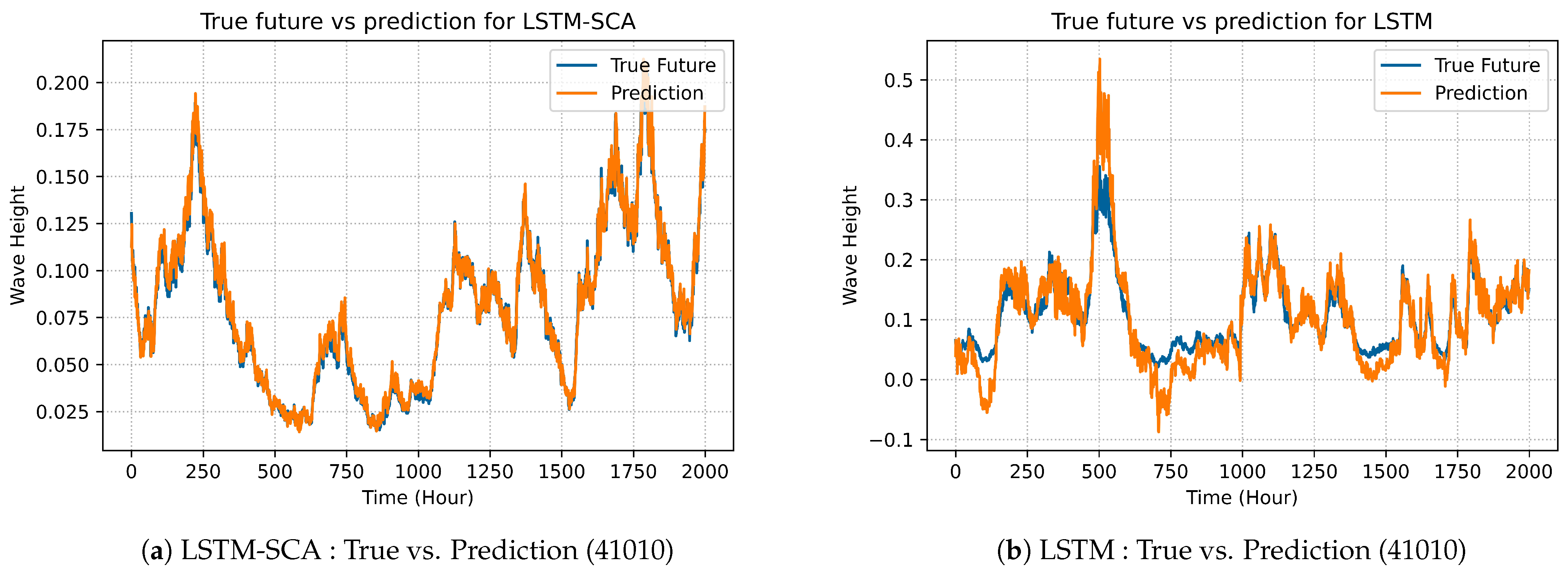
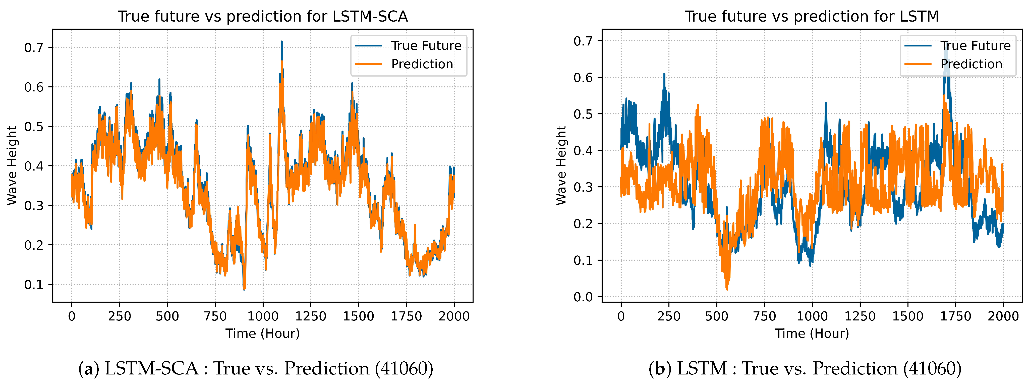
LSTM-SAC model’s best predicted results are illustrated in prediction graphs as shown in Figures 4a, 7a, 10a and 13a and compared with the best selected results of original LSTM, which are shown in Figures 4b, 7b, 10b and 13b.

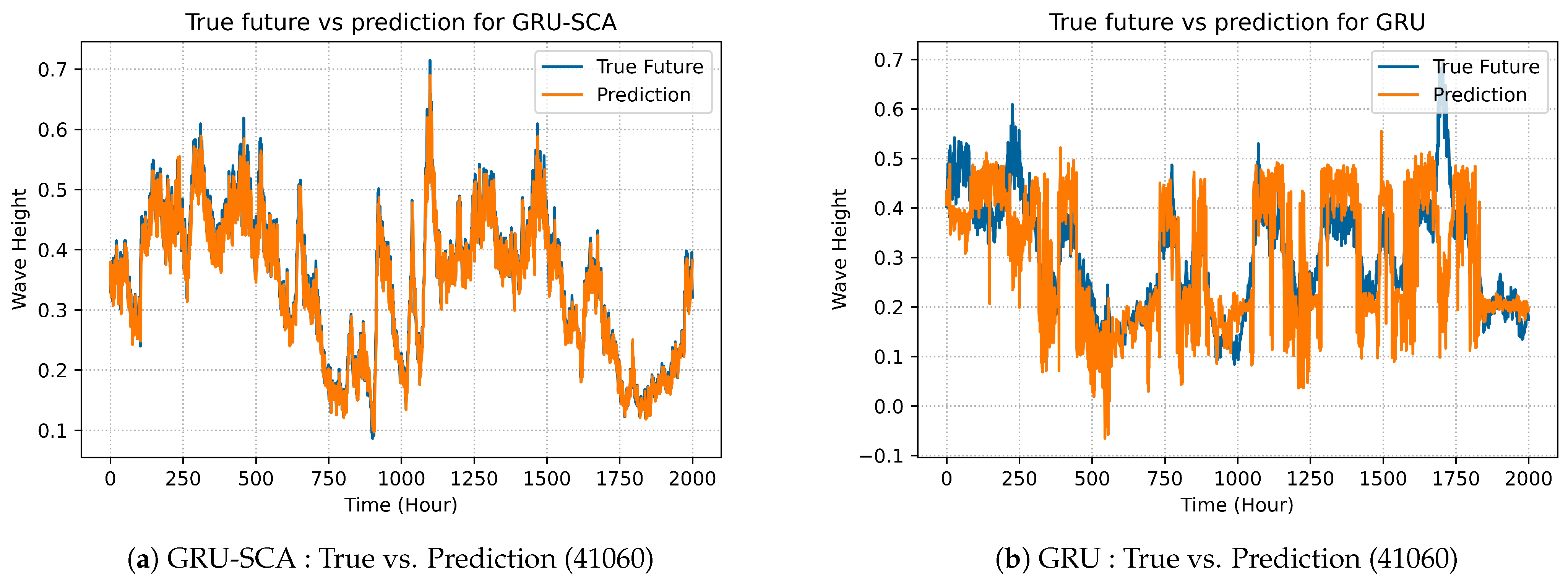
The best selected results produced by GRU-SCA can be seen in Figures 5a, 8a, 11a and 14a. On the other hand, Figures 5b, 8b, 11b and 14b show the results for the original GRU model.

7.3. Discussion

All experiments on the three models showed that our proposed technique can be effectively used to forecast wave heights with more prediction accuracy. The simple architecture of all variant of recurrent neural networks, which are VRNN, LSTM, and GRU, can be optimized in terms of weights generation by sine cosine optimization algorithm. The proposed RNN-SCA models have shown an outstanding performance and outperformed the state-of-the-art models in terms of MSE, RMSE, and MAE.

The difference between the graphs in Figure 3 is slightly noticeable. The enhanced model VRNN-SCA’s best prediction for dataset 41010 was in epoch 40 and is shown in Figure 3a. It is more accurate than original model (VRNN) prediction illustrated in Figure 3b. Similarly, Figure 4 shows the comparison over dataset 41010 in terms of prediction between the enhanced LSTM-SCA and original LSTM. As can be seen in Figure 4a, LSTM-SCA in epoch 40 produces the best results for predicating the wave heights. The results outperform and is more precise than that of original LSTM which is shown in Figure 4b. The performance of GRU-SCA is compared with the original GRU in terms of prediction as shown in Figure 5. As can be seen form Figure 5a, the best results among all models over dataset 41010 was for GRU-SCA with the value of $8.54\times {10}^{-5}$, which clearly outperform the original GRU shown in Figure 5b.

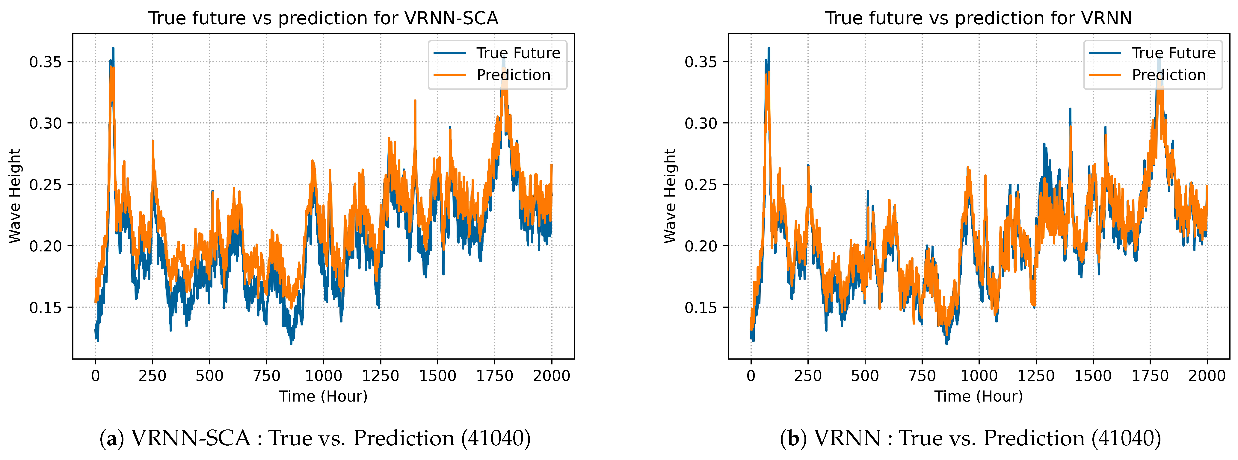
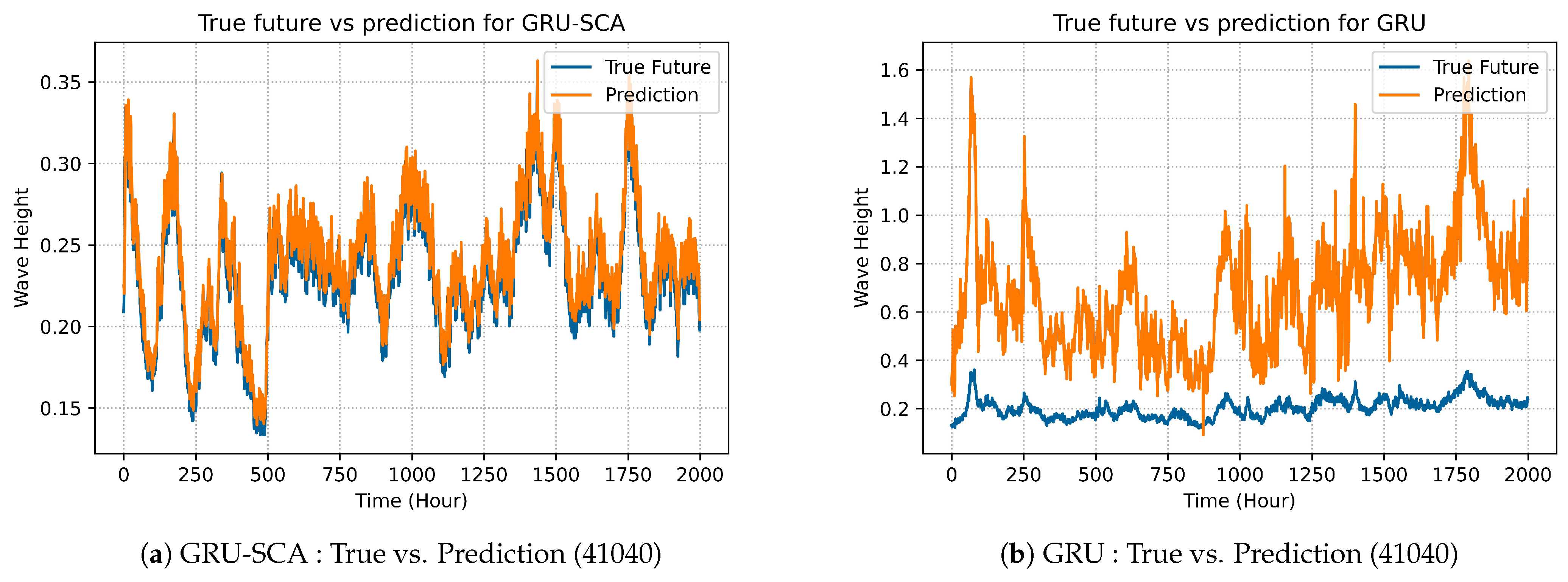
Figure 6 shows the comparison between the proposed VRNN-SCA and the original VRNN models in term of prediction for dataset form station 41040. Figure 6a shows that the prediction of VRNN-SCA outperforms the original VRNN shown in Figure 6b. This is because the SCA algorithm is effective at producing better prediction accuracy compared to the original one. Similarly, Figure 7 shows the comparison between the proposed model LSTM-SCA and the original LSTM; the proposed model (Figure 7a) clearly outperforms the original one (Figure 7b) in terms of accurately predicating the wave heights. The performance of GRU-SCA is compared with the original GRU in terms of prediction as shown in Figure 8. As can be seen form Figure 8a, the best results among all models over dataset 41040 was for GRU-SCA, which clearly outperform the original GRU shown in Figure 8b.

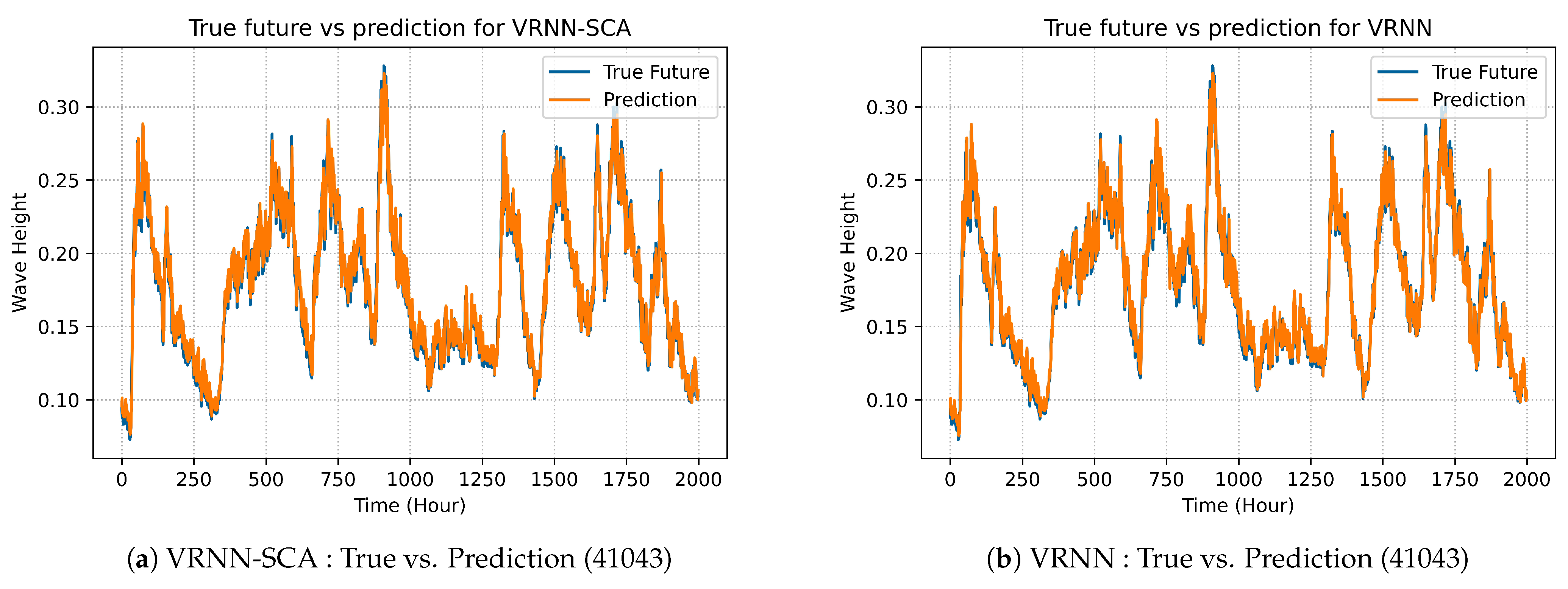
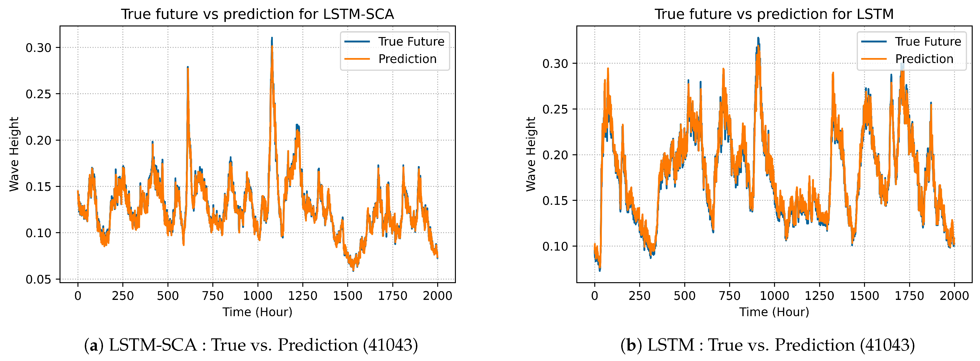
In Figure 9, there is the comparison between VRNN-SCA model and VRNN in terms of best prediction on dataset 41043. Figure 9a demonstrates the best prediction of the enhanced model VRNN-SCA, while Figure 9b explains the prediction of the original VRNN. The performance of LSTM-SCA on dataset 41043 is demonstrated in Figure 10a, similarly the performance of original LSTM is depicted on Figure 10b. Figure 11a demonstrates the prediction of the enhanced model GRU-SCA, whereas Figure 11b model’s prediction.

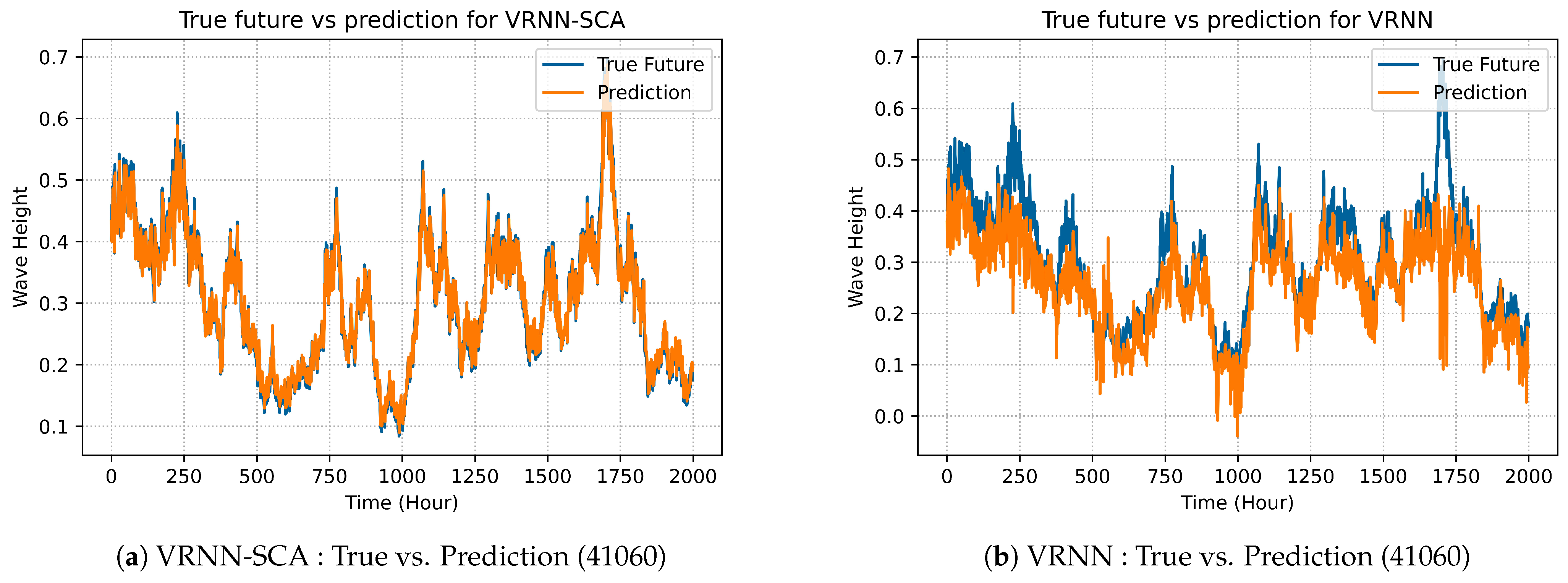
Figure 12 shows the comparison between the proposed VRNN-SCA and the original VRNN models in term of prediction for the dataset from station 41060. Figure 12a shows the prediction of VRNN-SCA outperforms the original VRNN showed in Figure 12b. Similarly, Figure 13 shows the comparison between the proposed model LSTM-SCA and the original LSTM; the proposed model (Figure 13a) clearly outperform the original one (Figure 13b) in terms of accurately predicate the wave heights. The performance of GRU-SCA is compared with the original GRU in terms of prediction as shown in Figure 14. As can be seen form Figure 14a, the best results among all models over dataset 41043 was for GRU-SCA, which clearly outperforms the original GRU shown in Figure 14b. This is due to the effective of the SCA algorithm in producing better prediction accuracy comparing to the original one.

The graphs give a clear point of view that experiments of the proposed models for all four datasets compared to the original models have more accurate prediction with minimum loss values. The datasets have different sizes and different variations of numbers in each year. The metrics used to evaluate the performance and prediction accuracy are MSE, RMSE, and MAE. As the experiments have been run in the interval of 10 epochs, we notice that every stop point has different values. These values improve as the epochs number increases. The best values for every metric in the table is highlighted in bold for each dataset.

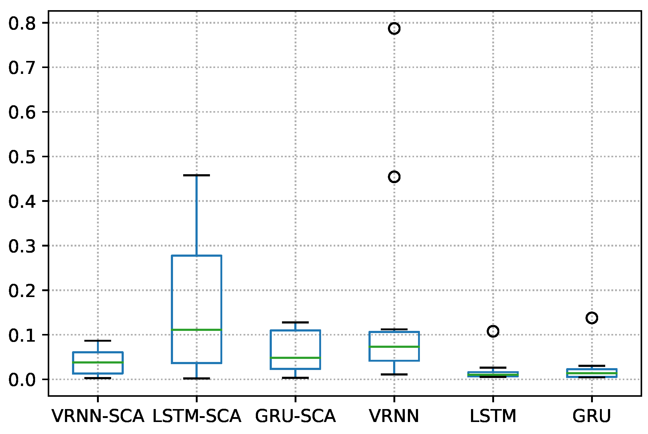
7.4. Significance Analysis

The one-way analysis of variance (ANOVA) test was used to assess the statistical significance of the differences between the resulting MSE obtained by proposed models versus other models. The findings of this analysis indicate whether the findings of the experiments are independent. No significance difference between the MSE of the proposed models and other models is assumed by the null hypothesis. The null hypothesis is accepted at state level greater than 0.05 and rejected at state level less than 0.05. ANOVA is an effective analysis technique as it accepts more than two groups to find the significance differences, and because we have six groups, the ANOVA test is selected. The procedures of this analysis are adopted from in [80].

In dataset 41010, the obtained p-value, as can be seen in

Table 14. ANOVA table results on dataset 41010.

Source	SS	df	MS	F	p-Value
Groups	14.6488	5	2.92975	8.91	0.000003
Error	17.7537	54	0.32877
Total	32.4025	59

, is 0.000003, which is less than 0.05, and we can thus reject the null hypothesis and indicate there is a significant difference between the proposed models and the original models. Figure 15 shows the boxplot of the differences between the proposed models and benchmarking models.

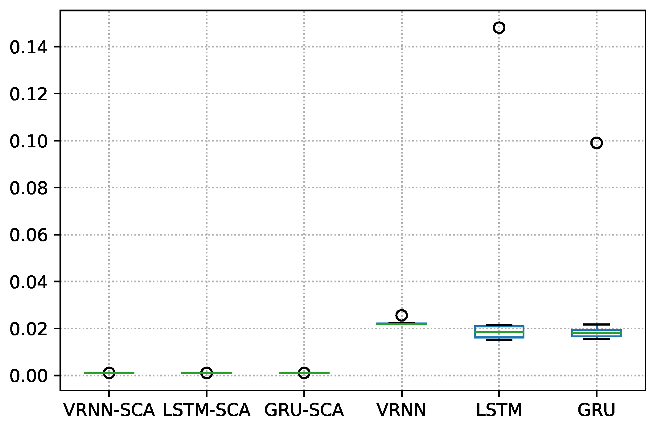
Similarly, in dataset 41040, the obtained p-value, as can be seen from

Table 15. ANOVA table results on the dataset 41040.

Source	SS	df	MS	F	p-Value
Groups	0.21364	5	0.04273	8.91	0.0000001
Error	0.24003	54	0.00445
Total	0.45368	59

, is 0.000001, which strongly indicates that there is a significance difference between the proposed models and original models. Figure 16 illustrates the boxplot of the differences between the proposed models and original models on this dataset.

For dataset 41043, there is a slight difference, and, as can be seen from

Table 16. ANOVA table results on dataset 41043.

Source	SS	df	MS	F	p-Value
Groups	0.23861	5	0.04772	3	0.0183
Error	0.85785	54	0.01589
Total	1.09646	59

, the obtained p-values is 0.0183, which still less than state level 0.05. Figure 17 demonstrates these difference as a boxplot.

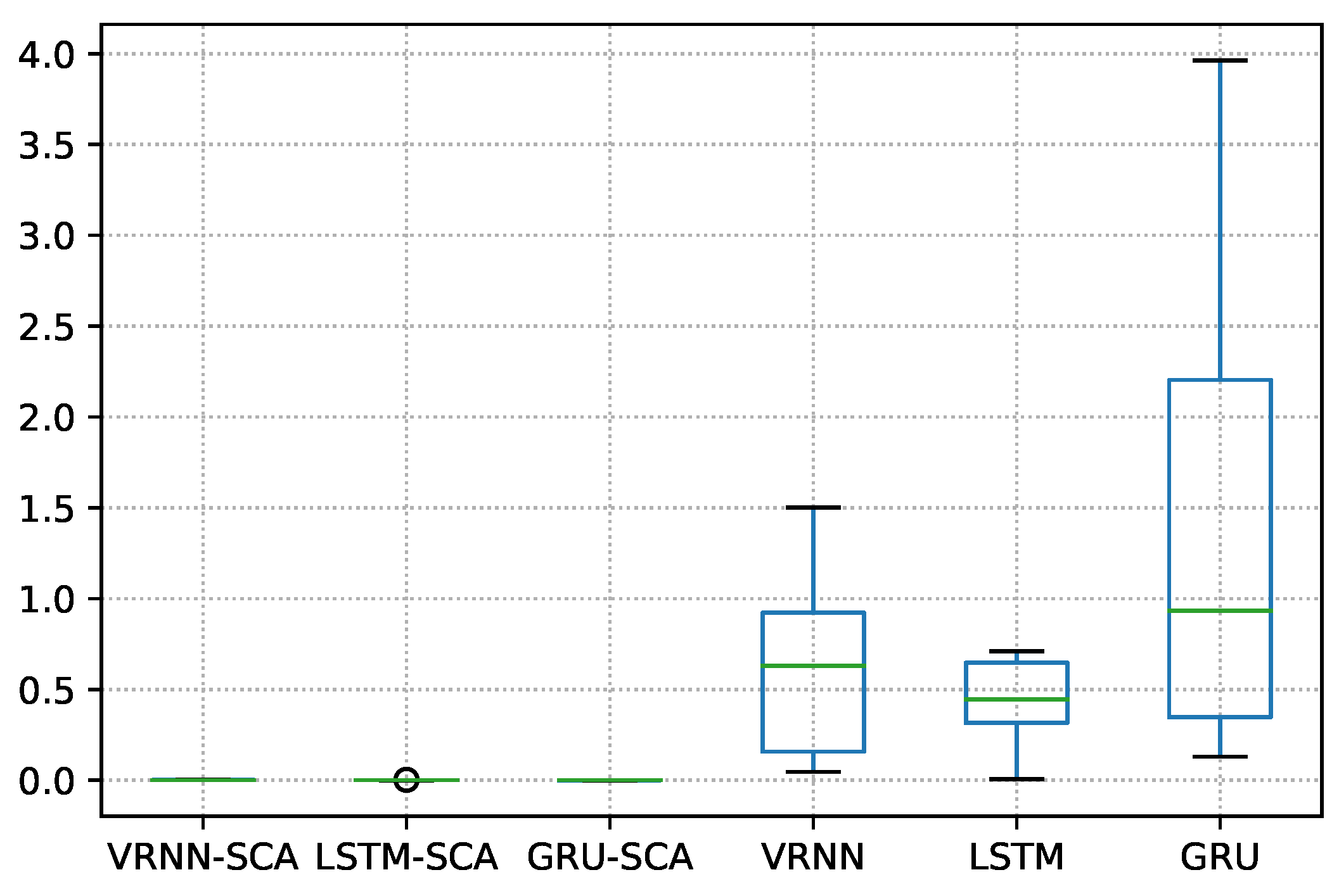
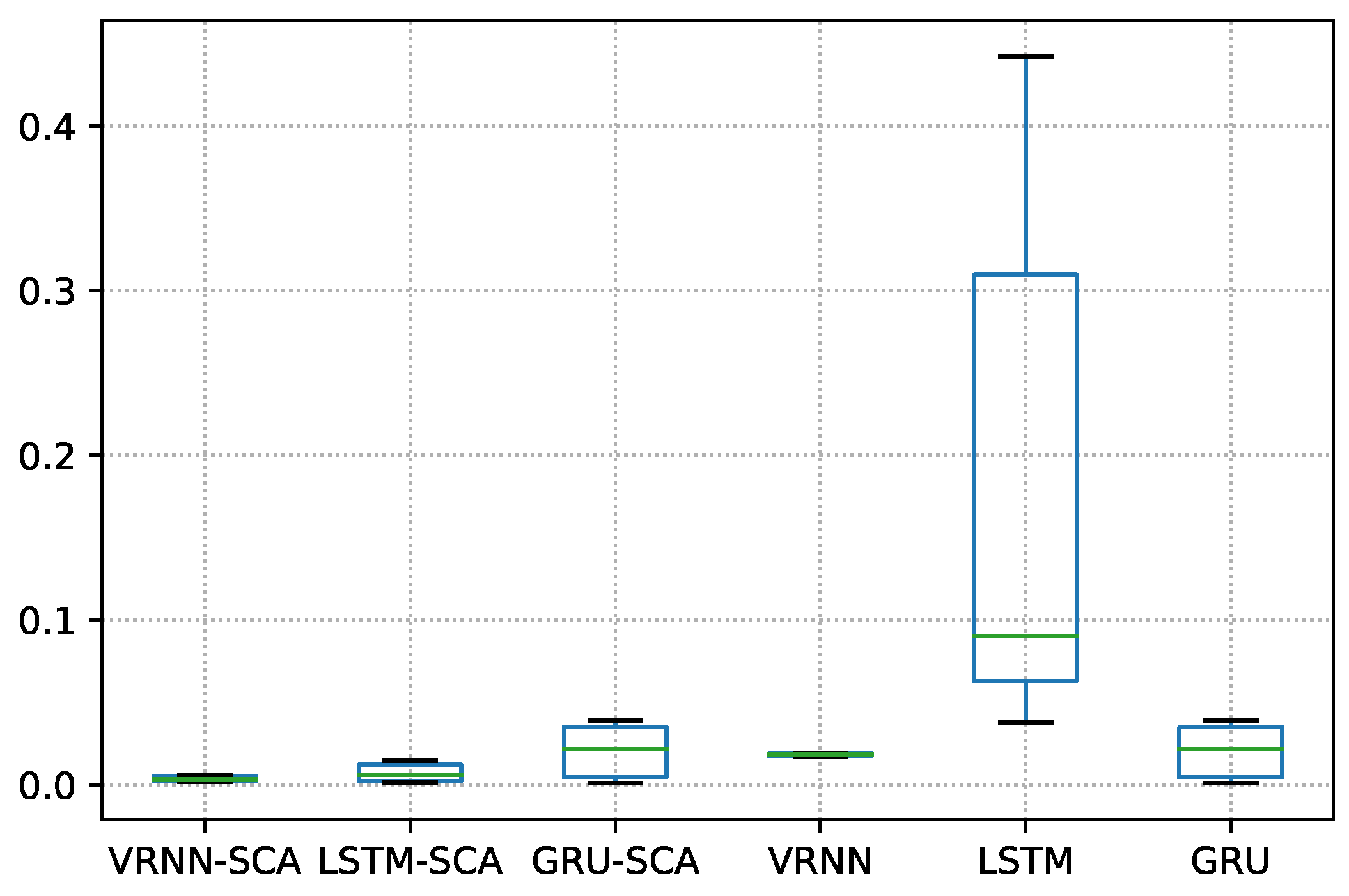
Finally, in dataset 41060, the obtained p-value, as shown in

Table 17. ANOVA table results on dataset 41060.

Source	SS	df	MS	F	p-Value
Groups	0.01017	5	0.00203	5.18	0.0006
Error	0.02118	54	0.00039
Total	0.03135	59

, is 0.0006, which demonstrates a strong indication of the superiority of the proposed models. Figure 18 illustrates the boxplot differences on this dataset.

8. Conclusions and Future Work

This paper proposed an enhanced weight-optimized recurrent neural network based on the sine cosine algorithm for predicting with high accuracy the wave heights. The proposed models’ structures were first configured with optimal hyperparameters using grid search technique. The grid search is used to find the best values for learning rate. Three models are proposed, namely VRNN-SCA, LSTM-SCA, and GRU-SCA, by integrating the sine cosine algorithm. The results proved that the proposed models have the capability of improving waves prediction and producing better results than original models. The results of the proposed models demonstrate much better results comparing the original ones, for example, the best averages MSE on 41010 datasets were 0.0003, 0.0005, and 0.0008 for GRU-SCA, LSTM-SCA, and VRNN-SCA, respectively, whereas the best average RMSE was 0.0165, 0.0205, and 0.0269 for GRU-SCA, LSTM-SCA, and VRNN-SCA, respectively. Similarly, the best average MAE for GRU-SCA, LSTM-SCA, and VRNN-SCA was 0.0113, 0.0130, and 0.0133, respectively.

The integration of SCA has helped the simple architectures of RNNs to generate weights that are adaptable to the selected data set and models structures. In traditional training of RNN, the initialization of weights happens randomly, ignoring the datasets size. This increases the possibility of the model vanishing, exploding, or becoming trapped in local optima. Therefore, our technique utilized the advantages of SCA by generating adaptive weight values that can adapted with the model’s parameters and the datasets simultaneously. The proposed VRNN-SCA, LSTM-SCA, and GRU-SCA models are effective tools in forecasting wave height and can be recommended to solve other prediction problems. In future work, according to the “No Free Lunch” theorem, other optimization algorithms such as gray wolf optimizer or dragonfly algorithm could be investigated to optimize the weight of recurrent neural networks. Besides, the proposed models could be investigated on other domains such as forecasting air pollution, flood prediction, and wind speed forecasting. Another future direction is to use different evaluation indices to validate the performance of models such as Moving Average, Weighted MA, or Exponential smoothing.

References

- Fan, S.; Xiao, N.; Dong, S. A novel model to predict significant wave height based on long short-term memory network. Ocean Eng. 2020, 205, 107298. [Google Scholar] [CrossRef]
- Jain, P.; Deo, M.; Latha, G.; Rajendran, V. Real time wave forecasting using wind time history and numerical model. Ocean Model. 2011, 36, 26–39. [Google Scholar] [CrossRef]
- Aderinto, T.; Li, H. Ocean wave energy converters: Status and challenges. Energies 2018, 11, 1250. [Google Scholar] [CrossRef]
- Abdulkadir, S.J.; Yong, S.P. Unscented kalman filter for noisy multivariate financial time-series data. In International Workshop on Multi-Disciplinary Trends in Artificial Intelligence; Springer: Berlin/Heidelberg, Germany, 2013; pp. 87–96. [Google Scholar]
- Aisjah, A.S.; Arifin, S.; Danistha, W.L. Sverdruv Munk Bretschneider Modification (SMB) for Significant Wave Height Prediction in Java Sea. Curr. J. Appl. Sci. Technol. 2016, 1–8. [Google Scholar] [CrossRef]
- McCormick, M. Wind-wave power available to a wave energy converter array. Ocean Eng. 1978, 5, 67–74. [Google Scholar] [CrossRef]
- Wang, W.; Tang, R.; Li, C.; Liu, P.; Luo, L. A BP neural network model optimized by Mind Evolutionary Algorithm for predicting the ocean wave heights. Ocean Eng. 2018, 162, 98–107. [Google Scholar] [CrossRef]
- Abdulkadir, S.J.; Yong, S.P. Scaled UKF–NARX hybrid model for multi-step-ahead forecasting of chaotic time series data. Soft Comput. 2015, 19, 3479–3496. [Google Scholar] [CrossRef]
- Alqushaibi, A.; Abdulkadir, S.J.; Rais, H.M.; Al-Tashi, Q. A Review of Weight Optimization Techniques in Recurrent Neural Networks. In Proceedings of the 2020 International Conference on Computational Intelligence (ICCI), Bandar Seri Iskandar, Malaysia, 8–9 October 2020; pp. 196–201. [Google Scholar] [CrossRef]
- Abdulkadir, S.J.; Yong, S.P.; Zakaria, N. Hybrid neural network model for metocean data analysis. J. Inform. Math. Sci. 2016, 8, 245–251. [Google Scholar]
- Alqushaibi, A.; Abdulkadir, S.J.; Rais, H.M.; Al-Tashi, Q.; Ragab, M.G. An Optimized Recurrent Neural Network for Metocean Forecasting. In Proceedings of the 2020 International Conference on Computational Intelligence (ICCI), Bandar Seri Iskandar, Malaysia, 8–9 October 2020; pp. 190–195. [Google Scholar] [CrossRef]
- An, P.; Liu, Q.; Abedi, F.; Yang, Y. Novel calibration method for camera array in spherical arrangement. Signal Process. Image Commun. 2020, 80, 115682. [Google Scholar] [CrossRef]
- Pradhan, R.; Aygun, R.S.; Maskey, M.; Ramachandran, R.; Cecil, D.J. Tropical cyclone intensity estimation using a deep convolutional neural network. IEEE Trans. Image Process. 2017, 27, 692–702. [Google Scholar] [CrossRef] [PubMed]
- Deo, M.; Naidu, C.S. Real time wave forecasting using neural networks. Ocean Eng. 1998, 26, 191–203. [Google Scholar] [CrossRef]
- Mandal, S.; Prabaharan, N. Ocean wave forecasting using recurrent neural networks. Ocean Eng. 2006, 33, 1401–1410. [Google Scholar] [CrossRef]
- Mahjoobi, J.; Mosabbeb, E.A. Prediction of significant wave height using regressive support vector machines. Ocean Eng. 2009, 36, 339–347. [Google Scholar] [CrossRef]
- Etemad-Shahidi, A.; Mahjoobi, J. Comparison between M5 model tree and neural networks for prediction of significant wave height in Lake Superior. Ocean Eng. 2009, 36, 1175–1181. [Google Scholar] [CrossRef]
- Azencott, R.; Muravina, V.; Hekmati, R.; Zhang, W.; Paldino, M. Automatic clustering in large sets of time series. In Contributions to Partial Differential Equations and Applications; Springer: Berlin/Heidelberg, Germany, 2019; pp. 65–75. [Google Scholar]
- Lehmann, M.; Karimpour, F.; Goudey, C.A.; Jacobson, P.T.; Alam, M.R. Ocean wave energy in the United States: Current status and future perspectives. Renew. Sustain. Energy Rev. 2017, 74, 1300–1313. [Google Scholar] [CrossRef]
- Pirhooshyaran, M.; Snyder, L.V. Forecasting, hindcasting and feature selection of ocean waves via recurrent and sequence-to-sequence networks. Ocean Eng. 2020, 207, 107424. [Google Scholar] [CrossRef]
- Tolman, H.L. A third-generation model for wind waves on slowly varying, unsteady, and inhomogeneous depths and currents. J. Phys. Oceanogr. 1991, 21, 782–797. [Google Scholar] [CrossRef]
- Kagemoto, H. Forecasting a water-surface wave train with artificial intelligence—A case study. Ocean Eng. 2020, 207, 107380. [Google Scholar] [CrossRef]
- Reikard, G.; Rogers, W.E. Forecasting ocean waves: Comparing a physics-based model with statistical models. Coast. Eng. 2011, 58, 409–416. [Google Scholar] [CrossRef]
- Abdulkadir, S.J.; Alhussian, H.; Nazmi, M.; Elsheikh, A.A. Long Short Term Memory Recurrent Network for Standard and Poor’s 500 Index Modelling. Int. J. Eng. Technol. 2018, 7, 25–29. [Google Scholar] [CrossRef]
- Abraham, B.; Ledolter, J. Statistical Methods for Forecasting; John Wiley & Sons: Hoboken, NJ, USA, 2009; Volume 234. [Google Scholar]
- Abdulkadir, S.J.; Yong, S.P.; Marimuthu, M.; Lai, F.W. Hybridization of ensemble Kalman filter and non-linear auto-regressive neural network for financial forecasting. In Mining Intelligence and Knowledge Exploration; Springer: Berlin/Heidelberg, Germany, 2014; pp. 72–81. [Google Scholar]
- Rasp, S.; Lerch, S. Neural networks for postprocessing ensemble weather forecasts. Mon. Weather Rev. 2018, 146, 3885–3900. [Google Scholar] [CrossRef]
- Campos, R.M.; Krasnopolsky, V.; Alves, J.H.; Penny, S.G. Improving NCEP’s global-scale wave ensemble averages using neural networks. Ocean Model. 2020, 149, 101617. [Google Scholar] [CrossRef]
- Harpham, Q.; Tozer, N.; Cleverley, P.; Wyncoll, D.; Cresswell, D. A Bayesian method for improving probabilistic wave forecasts by weighting ensemble members. Environ. Model. Softw. 2016, 84, 482–493. [Google Scholar] [CrossRef]
- Campos, R.M.; Krasnopolsky, V.; Alves, J.H.G.; Penny, S.G. Nonlinear wave ensemble averaging in the Gulf of Mexico using neural networks. J. Atmos. Ocean. Technol. 2019, 36, 113–127. [Google Scholar] [CrossRef]
- Durrant, T.H.; Woodcock, F.; Greenslade, D.J. Consensus forecasts of modeled wave parameters. Weather Forecast. 2009, 24, 492–503. [Google Scholar] [CrossRef]
- Özger, M. Prediction of ocean wave energy from meteorological variables by fuzzy logic modeling. Expert Syst. Appl. 2011, 38, 6269–6274. [Google Scholar] [CrossRef]
- Zhang, Y.; Liu, R.; Wang, X.; Chen, H.; Li, C. Boosted binary Harris hawks optimizer and feature selection. Eng. Comput. 2020, 1–30. [Google Scholar] [CrossRef]
- Al-Tashi, Q.; Rais, H.M.; Abdulkadir, S.J.; Mirjalili, S.; Alhussian, H. A review of grey wolf optimizer-based feature selection methods for classification. In Evolutionary Machine Learning Techniques; Springer: Berlin/Heidelberg, Germany, 2020; pp. 273–286. [Google Scholar]
- Al-Wajih, R.; Abdulkadir, S.J.; Aziz, N.; Al-Tashi, Q.; Talpur, N. Hybrid Binary Grey Wolf With Harris Hawks Optimizer for Feature Selection. IEEE Access 2021, 9, 31662–31677. [Google Scholar] [CrossRef]
- Balogun, A.O.; Basri, S.; Mahamad, S.; Abdulkadir, S.J.; Almomani, M.A.; Adeyemo, V.E.; Al-Tashi, Q.; Mojeed, H.A.; Imam, A.A.; Bajeh, A.O. Impact of feature selection methods on the predictive performance of software defect prediction models: An extensive empirical study. Symmetry 2020, 12, 1147. [Google Scholar] [CrossRef]
- Al-Tashi, Q.; Abdulkadir, S.J.; Rais, H.M.; Mirjalili, S.; Alhussian, H. Approaches to multi-objective feature selection: A systematic literature review. IEEE Access 2020, 8, 125076–125096. [Google Scholar] [CrossRef]
- Deo, M.C.; Jha, A.; Chaphekar, A.; Ravikant, K. Neural networks for wave forecasting. Ocean Eng. 2001, 28, 889–898. [Google Scholar] [CrossRef]
- Alexandre, E.; Cuadra, L.; Nieto-Borge, J.; Candil-Garcia, G.; Del Pino, M.; Salcedo-Sanz, S. A hybrid genetic algorithm—Extreme learning machine approach for accurate significant wave height reconstruction. Ocean Model. 2015, 92, 115–123. [Google Scholar] [CrossRef]
- Zhang, Y.; Liu, R.; Heidari, A.A.; Wang, X.; Chen, Y.; Wang, M.; Chen, H. Towards augmented kernel extreme learning models for bankruptcy prediction: Algorithmic behavior and comprehensive analysis. Neurocomputing 2021, 430, 185–212. [Google Scholar] [CrossRef]
- Zhao, D.; Liu, L.; Yu, F.; Heidari, A.A.; Wang, M.; Liang, G.; Muhammad, K.; Chen, H. Chaotic random spare ant colony optimization for multi-threshold image segmentation of 2D Kapur entropy. Knowl. Based Syst. 2020, 216, 106510. [Google Scholar] [CrossRef]
- Tu, J.; Chen, H.; Liu, J.; Heidari, A.A.; Zhang, X.; Wang, M.; Ruby, R.; Pham, Q.V. Evolutionary biogeography-based whale optimization methods with communication structure: Towards measuring the balance. Knowl. Based Syst. 2021, 212, 106642. [Google Scholar] [CrossRef]
- Wang, M.; Chen, H. Chaotic multi-swarm whale optimizer boosted support vector machine for medical diagnosis. Appl. Soft Comput. 2020, 88, 105946. [Google Scholar] [CrossRef]
- Shan, W.; Qiao, Z.; Heidari, A.A.; Chen, H.; Turabieh, H.; Teng, Y. Double adaptive weights for stabilization of moth flame optimizer: Balance analysis, engineering cases, and medical diagnosis. Knowl. Based Syst. 2020, 214, 106728. [Google Scholar] [CrossRef]
- Xu, Y.; Chen, H.; Luo, J.; Zhang, Q.; Jiao, S.; Zhang, X. Enhanced Moth-flame optimizer with mutation strategy for global optimization. Inf. Sci. 2019, 492, 181–203. [Google Scholar] [CrossRef]
- Wang, M.; Chen, H.; Yang, B.; Zhao, X.; Hu, L.; Cai, Z.; Huang, H.; Tong, C. Toward an optimal kernel extreme learning machine using a chaotic moth-flame optimization strategy with applications in medical diagnoses. Neurocomputing 2017, 267, 69–84. [Google Scholar] [CrossRef]
- Chen, H.; Heidari, A.A.; Chen, H.; Wang, M.; Pan, Z.; Gandomi, A.H. Multi-population differential evolution-assisted Harris hawks optimization: Framework and case studies. Future Gener. Comput. Syst. 2020, 111, 175–198. [Google Scholar] [CrossRef]
- Savitha, R.; Al Mamun, A. Regional ocean wave height prediction using sequential learning neural networks. Ocean Eng. 2017, 129, 605–612. [Google Scholar]
- Akbarifard, S.; Radmanesh, F. Predicting sea wave height using Symbiotic Organisms Search (SOS) algorithm. Ocean Eng. 2018, 167, 348–356. [Google Scholar] [CrossRef]
- Mnasri, S.; Nasri, N.; Van den Bossche, A.; Val, T. A new multi-agent particle swarm algorithm based on birds accents for the 3D indoor deployment problem. ISA Trans. 2019, 91, 262–280. [Google Scholar] [CrossRef] [PubMed]
- Cerqueira, V.; Torgo, L.; Smailović, J.; Mozetič, I. A comparative study of performance estimation methods for time series forecasting. In Proceedings of the 2017 IEEE International Conference on Data Science and Advanced Analytics (DSAA), Tokyo, Japan, 19–21 October 2017; pp. 529–538. [Google Scholar]
- Bergmeir, C.; Hyndman, R.J.; Koo, B. A note on the validity of cross-validation for evaluating autoregressive time series prediction. Comput. Stat. Data Anal. 2018, 120, 70–83. [Google Scholar] [CrossRef]
- Rashid, T.A.; Fattah, P.; Awla, D.K. Using accuracy measure for improving the training of LSTM with metaheuristic algorithms. Procedia Comput. Sci. 2018, 140, 324–333. [Google Scholar] [CrossRef]
- Somu, N.; MR, G.R.; Ramamritham, K. A hybrid model for building energy consumption forecasting using long short term memory networks. Appl. Energy 2020, 261, 114131. [Google Scholar] [CrossRef]
- Rosli, S.J.; Rahim, H.A.; Abdul Rani, K.N.; Ngadiran, R.; Ahmad, R.B.; Yahaya, N.Z.; Abdulmalek, M.; Jusoh, M.; Yasin, M.N.M.; Sabapathy, T.; et al. A Hybrid Modified Method of the Sine Cosine Algorithm Using Latin Hypercube Sampling with the Cuckoo Search Algorithm for Optimization Problems. Electronics 2020, 9, 1786. [Google Scholar] [CrossRef]
- Al-Tashi, Q.; Abdulkadir, S.J.; Rais, H.M.; Mirjalili, S.; Alhussian, H.; Ragab, M.G.; Alqushaibi, A. Binary Multi-Objective Grey Wolf Optimizer for Feature Selection in Classification. IEEE Access 2020, 8, 106247–106263. [Google Scholar] [CrossRef]
- Al-Tashi, Q.; Kadir, S.J.A.; Rais, H.M.; Mirjalili, S.; Alhussian, H. Binary optimization using hybrid grey wolf optimization for feature selection. IEEE Access 2019, 7, 39496–39508. [Google Scholar] [CrossRef]
- Steele, K.; Teng, C.C.; Wang, D. Wave direction measurements using pitch-roll buoys. Ocean Eng. 1992, 19, 349–375. [Google Scholar] [CrossRef]
- Fernández, J.C.; Salcedo-Sanz, S.; Gutiérrez, P.A.; Alexandre, E.; Hervás-Martínez, C. Significant wave height and energy flux range forecast with machine learning classifiers. Eng. Appl. Artif. Intell. 2015, 43, 44–53. [Google Scholar] [CrossRef]
- Hashim, R.; Roy, C.; Motamedi, S.; Shamshirband, S.; Petković, D. Selection of climatic parameters affecting wave height prediction using an enhanced Takagi-Sugeno-based fuzzy methodology. Renew. Sustain. Energy Rev. 2016, 60, 246–257. [Google Scholar] [CrossRef]
- Salehinejad, H.; Sankar, S.; Barfett, J.; Colak, E.; Valaee, S. Recent advances in recurrent neural networks. arXiv 2017, arXiv:1801.01078. [Google Scholar]
- Alom, M.Z.; Taha, T.M.; Yakopcic, C.; Westberg, S.; Sidike, P.; Nasrin, M.S.; Hasan, M.; Van Essen, B.C.; Awwal, A.A.; Asari, V.K. A state-of-the-art survey on deep learning theory and architectures. Electronics 2019, 8, 292. [Google Scholar] [CrossRef]
- He, K.; Zhang, X.; Ren, S.; Sun, J. Delving deep into rectifiers: Surpassing human-level performance on imagenet classification. In Proceedings of the IEEE International Conference on Computer Vision, Santiago, Chile, 7–13 December 2015; pp. 1026–1034. [Google Scholar]
- Lipton, Z.C.; Berkowitz, J.; Elkan, C. A critical review of recurrent neural networks for sequence learning. arXiv 2015, arXiv:1506.00019. [Google Scholar]
- Hochreiter, S.; Schmidhuber, J. Long short-term memory. Neural Comput. 1997, 9, 1735–1780. [Google Scholar] [CrossRef]
- Werbos, P.J. Backpropagation through time: What it does and how to do it. Proc. IEEE 1990, 78, 1550–1560. [Google Scholar] [CrossRef]
- Abdulkadir, S.J.; Alhussian, H.; Alzahrani, A.I. Analysis of recurrent neural networks for henon simulated time-series forecasting. J. Telecommun. Electron. Comput. Eng. 2018, 10, 155–159. [Google Scholar]
- Cho, K.; Van Merriënboer, B.; Gulcehre, C.; Bahdanau, D.; Bougares, F.; Schwenk, H.; Bengio, Y. Learning phrase representations using RNN encoder-decoder for statistical machine translation. arXiv 2014, arXiv:1406.1078. [Google Scholar]
- Chung, J.; Gulcehre, C.; Cho, K.; Bengio, Y. Empirical evaluation of gated recurrent neural networks on sequence modeling. arXiv 2014, arXiv:1412.3555. [Google Scholar]
- Mirjalili, S. SCA: A sine cosine algorithm for solving optimization problems. Knowl. Based Syst. 2016, 96, 120–133. [Google Scholar] [CrossRef]
- Attia, A.F.; El Sehiemy, R.A.; Hasanien, H.M. Optimal power flow solution in power systems using a novel Sine-Cosine algorithm. Int. J. Electr. Power Energy Syst. 2018, 99, 331–343. [Google Scholar] [CrossRef]
- Cherkassky, V.; Ma, Y. Selection of meta-parameters for support vector regression. In International Conference on Artificial Neural Networks; Springer: Berlin/Heidelberg, Germany, 2002; pp. 687–693. [Google Scholar]
- Hsu, C.W.; Chang, C.C.; Lin, C.J. A practical guide to support vector classification. Precis. Agric. 2003. [Google Scholar] [CrossRef]
- Feng, G.H. Support Vector Machine parameter selection method. Comput. Eng. Ring Appl. 2011, 47, 123. [Google Scholar]
- Hinz, T.; Navarro-Guerrero, N.; Magg, S.; Wermter, S. Speeding up the hyperparameter optimization of deep convolutional neural networks. Int. J. Comput. Intell. Appl. 2018, 17, 1850008. [Google Scholar] [CrossRef]
- Shuai, Y.; Zheng, Y.; Huang, H. Hybrid Software Obsolescence Evaluation Model Based on PCA-SVM-GridSearchCV. In Proceedings of the 2018 IEEE 9th International Conference on Software Engineering and Service Science (ICSESS), Beijing, China, 23–25 November 2018; pp. 449–453. [Google Scholar]
- Ragab, M.G.; Abdulkadir, S.J.; Aziz, N.; Al-Tashi, Q.; Alyousifi, Y.; Alhussian, H.; Alqushaibi, A. A Novel One-Dimensional CNN with Exponential Adaptive Gradients for Air Pollution Index Prediction. Sustainability 2020, 12, 10090. [Google Scholar] [CrossRef]
- Ragab, M.G.; Abdulkadir, S.J.; Aziz, N. Random Search One Dimensional CNN for Human Activity Recognition. In Proceedings of the 2020 International Conference on Computational Intelligence (ICCI), Bandar Seri Iskandar, Malaysia, 8–9 October 2020; pp. 86–91. [Google Scholar]
- Cao, W.; Wang, X.; Ming, Z.; Gao, J. A review on neural networks with random weights. Neurocomputing 2018, 275, 278–287. [Google Scholar] [CrossRef]
- Al-Tashi, Q.; Rais, H.M.; Abdulkadir, S.J.; Mirjalili, S. Feature Selection Based on Grey Wolf Optimizer for Oil & Gas Reservoir Classification. In Proceedings of the 2020 International Conference on Computational Intelligence (ICCI), Bandar Seri Iskandar, Malaysia, 8–9 October 2020; pp. 211–216. [Google Scholar]
Figure 1.
Stations’ location in the map.
Figure 2.
General model of the proposed RNN-SCA method.
Figure 3.
Comparison of VRNN models on dataset 41010.
Figure 4.
Comparison of LSTM models on dataset 41010.
Figure 5.
Comparison of GRU models on dataset 41010.
Figure 6.
Comparsion of VRNN models on dataset 41040.
Figure 7.
Comparison of LSTM models on dataset 41040.
Figure 8.
Comparison of GRU models on dataset 41040.
Figure 9.
Comparison of VRNN models on dataset 41043.
Figure 10.
Comparison of LSTM models on dataset 41043.
Figure 11.
Comparison of GRU models on dataset 41043.
Figure 12.
Comparison of VRNN models on dataset 41060.
Figure 13.
Comparison of LSTM models on dataset 41060.
Figure 14.
Comparison of GRU models on dataset 41060.
Figure 15.
Boxplot differences on the 41010 dataset.
Figure 16.
Boxplot differences on the 41040 dataset.
Figure 17.
Boxplot differences on the 41043 dataset.
Figure 18.
Boxplot differences on the 41060 dataset.