Abstract
Ports constitute a significant influence in the economic activity in coastal areas through operations and infrastructures to facilitate land and maritime transport of cargo. Ports are located in a multi-dimensional environment facing ocean and river hazards. Higher warming scenarios indicate Europe’s ports will be exposed to higher risk due to the increase in extreme sea levels (ESL), a combination of the mean sea level, tide, and storm surge. Located on the west Iberia Peninsula, the Aveiro Port is located in a coastal lagoon exposed to ocean and river flows, contributing to higher flood risk. This study aims to assess the flood extent for Aveiro Port for historical (1979–2005), near future (2026–2045), and far future (2081–2099) periods scenarios considering different return periods (10, 25, and 100-year) for the flood drivers, through numerical simulations of the ESL, wave regime, and riverine flows simultaneously. Spatial maps considering the flood extent and calculated area show that most of the port infrastructures’ resilience to flooding is found under the historical period, with some marginal floods. Under climate change impacts, the port flood extent gradually increases for higher return periods, where most of the terminals are at high risk of being flooded for the far-future period, whose contribution is primarily due to mean sea-level rise and storm surges.
1. Introduction
Maritime ports are major hubs of economic activity and are usually located in protected areas with access to navigable waterways due to marine transportation’s operational characteristics. Maritime trade has been increasing consistently with an annual average growth of 3.4% and a 4.7% increase in container port traffic [1], and even with the 2020 global pandemics contractions, the growth rate is expected to be recovered in 2021 [2]. Ports’ primary functions are to supply services to freight and ships and cover a wide range of functions that involve port operability. For instance, cargo-oriented infrastructures have been developed and expanded to new inland areas contiguous to the port to facilitate land and maritime transport systems in order to sustain the planned longevity of the infrastructural assets of about 40–50 years [3]. These characteristics turn the ports susceptible to complex dynamics of the multi-dimensional environmental [4,5] on which they are located, from the ocean (sea levels, storm surges, and sea weather) to rivers that can annihilate the ability to maintain the port activities efficiently.
Unprecedented climate change is occurring changing meteocean patterns around the globe [6,7,8,9], and recent studies show no signs of deceleration with sea-level rise exceeding 2 m [10,11] under higher emission scenarios, surpassing the IPCC AR5 [12] projections, with the potential to increase the vulnerability of coastal regions to floods. The Integrated Climate Data Center (ICDC) of the University of Hamburg determined the predicted relative sea level data that support the global estimates of the fifth IPCC report. The relative sea level includes surface mass balance and dynamic ice sheet contributions from Greenland and Antarctica, a glacier contribution, a land water storage contribution, glacial isostatic adjustment (GIA), and the inverse barometer effect (IBE). However, these projections do not consider the vertical land motion, whose long-term influence can be substantial and affect the regional mean sea level changes [13] and show significant variability in temporal and spatial evolution of the predicted mean sea levels [13,14,15].
Wind and wave regimes are expected to be affected [16] by climate change, along with weather events becoming more extreme [17,18]. The global climate models (GCMs) from Phase 5 of the Coupled Model Intercomparison Project (CMIP5) are a reliable source for the future ocean and atmospheric variables [15,19,20]. Drawing on the above, the United Nations (UN), governments, and the scientific community have been leaning forward on reverting the rise of carbon dioxide levels to tackle climate change impacts, which would require achieving net-zero greenhouse gas emission [21]. Such initiatives are of paramount importance to strengthen the global response to deal with climate change impacts. The European Commission supports the UN efforts through relevant legislation and climate strategies seeking to minimize risks to climate (a complete summary can be found in [22]). In addition, the European Union (EU) is highly dependent on port operation, with 75% of goods being imported and exported and 37% within the EU [23].
Given the ports’ location and the role in the globalized trading system, port adaptation and building their resilience to climate change is an urgent problem to be countered. Studies focusing on the European ports [24,25] showed that high warming scenarios (Representative Concentration Pathway—RCP8.5) indicate Europe’s ports will be exposed to higher risk, where most of the ports exposed to extreme sea levels (ESL) higher than 4.5 m in 2100 are located in the Iberian Peninsula (IP) [24]. Direct consequences on the number of trading goods could be affected, with an estimated cargo reduction of 25%. Broader impacts are expected since most IP port operations are performed in low-lying areas contiguous to the ports. Thus, acknowledge the extent of flooding under climate change is critical to enhancing flood resilience once ports are exposed to climate change impacts.
The west IP coast features several ports that provide an important gateway for Europe and Asia for trading and are vital for Portugal and Spain’s national economies [26]. This coast is characterized by highly variable coastal systems (estuaries, Rias, and lagoons), namely the Aveiro Lagoon that shelters the Aveiro Port. Due to its location and characteristics, the infrastructures of this port are prone to floods under the present climate [27,28,29], where a large extension of the surrounding areas of the port is flooded [29] under extreme sea levels. Flood assessment under future climate was addressed for the Aveiro Lagoon [30] but did not focus on the Aveiro Port, where a detailed assessment should be addressed by increasing the reliability and accuracy through modeling considering climate projections, which may be aggravated in the future due to climate change and may threaten the port’s performance. However, climate change impacts have not been assessed for Aveiro Port infrastructures inside its jurisdiction area. Thus, the present paper aims to assess the flooding conditions in Aveiro Port in response to climate change drivers through a detailed modeling study that quantifies the flooded area in a reference scenario that represents the present conditions and in climate change scenarios for the 10-, 25-, and 100-year return period (from now on referred to as Tr10, Tr25, and Tr100, respectively). The flood assessment will be determined by the simulation of the ESL (mean sea level, tide, and storm surge) simultaneously with wave regime as the ocean drivers and the riverine flows.
2. Study Area
2.1. Ria de Aveiro
Ria de Aveiro, an inland lagoon, is located on the IP west coast facing the Atlantic Ocean (40°39′ N, 8°45′ W), in Portugal (Figure 1a). The lagoon is comprised of four main channels (Mira, Ílhavo, Espinheiro, and S. Jacinto) and a single artificial channel connecting the lagoon to the Atlantic Ocean [30]. The elongated lagoon up to 45 km in length lies behind sandy barriers and extends up to 10 km onshore, covers an area of 89.2 km2 at spring tide, which is reduced to 64.9 km2 at neap tide [28]. An average depth of 1 m characterizes the lagoon due to the predominance of small channels, large areas of mudflats and salt marshes, and up to 15 m at the entrance and port area [29]. The region surrounding the lagoon is characterized by a low topography, which increases the potential to be flooded during certain conditions.
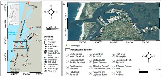
Figure 1.
Study area with the in situ stations (a) used to validate the hydrodynamic model. Location of the Aveiro Port and the business areas in the port administration jurisdiction (b).
The tide is the most important among the lagoon dynamic drivers, characterized by a semidiurnal regime with a small diurnal pattern, reaching average tidal amplitudes of 0.46 m at the neap tide and 3.52 m at spring tide. Several rivers also contribute to local hydrodynamics, with five major sources (Vouga, Antuã, Ribeira dos Moínhos, Cáster, and Boco rivers), where the Vouga river is the main contributor reaching a mean discharge of 80 m3/s [31]. These characteristics turn the lagoon vertically homogeneous, except during high inflows of fresh water in the channel’s upper part, where some vertical stratification is found [32,33].
With a northwest regime, the coastal waves are characterized by a mean significant wave height of 2 m and a mean wave period of 12 s, increasing significantly in winter, reaching 8 m during 5-day storm events [34]. Despite these high wave heights, studies showed that the presence of breakwaters along the lagoon mouth diminishes the influence of the waves at the entrance, slightly affecting the currents and sea level at the port operation areas [35,36]. In addition, storm surges can occur during adverse weather conditions, leading to an over-elevation ranging from 0.3 to 1.1 m [27,30,37].
The changes occurring in meteocean drivers contribute to the increase in the lagoon’s flood risk, which has been assessed for the historical period [27,29,38,39] to understand and predict future developments [28,30,35] of the flooded area and the implications on the surroundings. The Aveiro Lagoon has been historically shaped by human activities, harboring urban structures of small to medium-sized cities and related activities and increasing industrialization prompted by the Aveiro Port [40], which is particularly prone to floods due to the proximity of the lagoon mouth. These regions have been well documented in terms of floods, however, the potential impact of floods in future scenarios of climate change has not yet been assessed in detail for the Aveiro Port area, and particularly regarding the area of jurisdiction and the port infrastructures.
2.2. Aveiro Port
The Aveiro Port’s strategic location (40°39′ N, 8°45′ W) and its favorable maritime and land accessibilities allow this infrastructure to serve a vast economic hinterland in Portugal and central Spain. This port is the most recent national infrastructure, showing a well-ordered and integrated area, benefiting from the natural protection from the coastal hazards bestowed by the sandy barriers. In fact, the port structure lies inside Ria de Aveiro, and the connection between the port and the ocean is carried out by a single navigation channel protected by the construction of two breakwaters. These engineering works extend seaward, both north with an extension of 1200 m and south with 700 m, securing a 500 m wide entrance and narrowing to a 300 m wide channel to the port facilities.
Following [35,36], waves are expected to play a significant role in the lagoon inlet’s sea surface height, affecting currents and mean sea level near the entrance channel. Moreover, the breakwaters’ orientation is the port’s most crucial coastal defense structure, protecting the navigation channel from wave actions even during storms with extreme waves [36]. The inlet features allow achieving the channel’s required depth and stability even during rough winters, being a good shelter during these periods. However, low amplitude waves have been observed visually in the entrance channel between both breakwaters.
Such features attract large ships with a length up to 200 m and an average draft up to 9.75 m through the port entrance, located 2.4 km from the north sector (North Terminal; Container and Roll-on/Roll-off Terminal; Solid Bulk Cargo and Liquid Bulk Cargo Terminal) and 7.2 km from the south sector (South Terminal, High Sea Fishing Port and Specialized Fisheries Terminal) (Figure 1b) (portodeaveiro.pt, accessed on 27 February 2021).
3. Data and Methods
As mean sea-level rise and storms become more intense, the prediction of these drivers becomes essential to address the climate change impacts in Aveiro Port, which is susceptible to be flooded due to its location. The flood hazard is correlated to the intensity and periodicity of the drivers (relative sea level, storm surge, riverine flows, and wave-induced currents), showing higher hazard when the combination of several drivers reach their highest values. However, these assessments are only approachable through numerical models. DELFT3D is a software suite for a multi-disciplinary approach that allows carrying outflow and wave simulations in coastal, river, and estuarine areas. DELFT3D suite comprises several modules, such as the FLOW and WAVE, which simulate the flow and short-wave propagation. A model simulation’s fate is mainly determined by the inputs, reflecting the model’s accuracy to specific physical processes. These processes must be evaluated and determined, focusing on assessing the Aveiro Port’s flood rate, which strongly depends on high sea levels and riverine flows. Hence, each climate period’s return values were calculated by fitting the generalized Pareto distribution (GPD) to identify each driver’s extreme values by assuming stationary signals. These inputs will feed the hydrodynamic model in order to simulate several climate change scenarios under RCP8.5. Despite being described as a low possibility, it is also linked to a high-impact case [10,41] and describes the worst possible flood scenario, including a reference scenario representing the present climate.
3.1. Tide, Storm Surge, and Mean Sea Level
Coastal flooding is linked to storm surge events, generating an abnormal rise of the mean sea level above the predicted astronomical tide. When storm surge and high tides coincide, it can cause extreme flooding in these regions [29,30]. Climate change can worsen these events due to the predicted mean sea-level rise in the upcoming years [6,10,35].
This work uses the ESL determined by Lopes et al. [29] for the Historical period (Table 1) and considers an additional rise in MSL of 0.19 m and 0.68 m for near future and far future, respectively, that were obtained for the RCP8.5 by analyzing sea level variations for the Portuguese Coast for the periods 2026–2045 and 2081–2099. Sea level data correspond to an ensemble mean of 21 CMIP5 AOGCMs (Atmosphere-Ocean General Circulation Models) that support the global estimates of the fifth IPCC report. These data are accessible through the LAS (Live Access Server) interface of the Integrated Climate Data Center (ICDC) of the University of Hamburg (https://icdc.cen.uni-hamburg.de/1/daten/ocean/ar5-slr.html, accessed on 27 February 2021). It is noteworthy that ESL was determined by applying the joint probability approach to water level recorded at the lagoon mouth (Figure 1b) (for a detailed methodology, the reader is referred to [29]). The reference considers a tide reaching the level of mean high water springs (3.3 m) at the present mean sea level (MSL) [29]. The same approach was conducted to determine the ESL for the future periods considering that mean sea-level rise dominates the increase in floods, and storm surge heights and tides are expected to be minimal [42,43,44].

Table 1.
The return period of 10- (Tr10), 25- (Tr25), and 100- year (Tr100), and reference for extreme sea levels (meters) with the predicted sea-level rise and considering a simultaneously high tide and storm surge.
The ESL uncertainty relative to vertical land motion is residual in Aveiro Port location, showing relatively small vertical velocities in the region [13], and therefore, relatively low impacts on ESL for the end of the century, exhibiting ESL values of around 5 m [15], similar to the far future scenarios (Table 1).
Attending this, a similar approach to [30] was conducted to construct a time series to be used at the ocean boundary of the hydrodynamic model, taking into account the sea level evolution and a storm surge event coincident with high tide. For this purpose, the tidal constants of 2019 obtained from the tidal gauge (Figure 1b) located at the lagoon entrance were used to reconstruct the tide signal in order to determine the tidal range and the level of mean high water springs (for a detailed methodology the reader is referred to [29,30]). The same approach was conducted to determine the ESL for the future periods considering that mean sea-level rise dominates the increase in floods, and storm surge heights and tides are expected to be minimal [42,43,44]. The reference considers a tide reaching the level of mean high water springs (3.3 m) at the present mean sea level (MSL) (Table 1). The values for near future and far future horizons consider an MSL rise of 0.19 m and 0.68 m, respectively, that were obtained for the RCP8.5 by analyzing sea level variations for the Portuguese Coast for the periods 2026–2045 and 2081–2099. Sea level data correspond to an ensemble mean of 21 CMIP5 AOGCMs (Atmosphere-Ocean General Circulation Models) that support the global estimates of the fifth IPCC report. These data are accessible through the LAS (Live Access Server) interface of the Integrated Climate Da-ta Center (ICDC) of the University of Hamburg (https://icdc.cen.uni-hamburg.de/1/daten/ocean/ar5-slr.html, accessed on 27 February 2021).
3.2. River Discharge
Concerning the river discharges, the various discharges’ lack of continuous monitoring data led to modeled outputs from the SWAT model [45] at the five discharges. This model was previously calibrated and validated by [46]. The daily values obtained over 1931–2010 were used to determine the maximum annual discharges and fitted to statistical distributions (Generalized Extreme Value (GEV), Gamma, Log-n, Exponential, Gumbel, and Weibull). Then, the best distribution fit was determined by performing a chi-square goodness-of-fit test, Kolmogorov-Smirnov goodness-of-fit hypothesis test, and by computing the deviation between empirical and theoretical distributions. Finally, the best-fit distribution was used to estimate peak discharges for Tr10, Tr25, and Tr100 (Table 2). The reference case considers the mean value, which was determined based on the average discharge of the winter months (December, January, and February) for each tributary, taking into account the E-hype model outputs available online (https://hypeweb.smhi.se/explore-water/historical-data/europe-time-series/, accessed on 27 February 2021).
Table 2.
River discharges (m3/s) for reference, and 10-, 25-, and 100-years return periods.
The river discharge for future climate for the RCP8.5 can be estimated by reducing about 11% and 21% by the mid and end-century (Table 3) in this region, respectively (https://hypeweb.smhi.se/explore-water/climate-impacts/europe-climate-impacts/, accessed on 27 February 2021). Hence, this reduction was considered similar to previous studies [47] for the near and far future periods.
Table 3.
River discharge prediction (%) in the study region for the mid and end-century.
3.3. Waves
3.3.1. Global Wave Database
The historical and future wave conditions were obtained from the Commonwealth Scientific and Industrial Research Organization (CSIRO) online database [48,49]. The database is comprised of a Global Wave Hindcast (1979–2010) simulated by the WAVEWATCH III (WWIII) version 4.08, forced with Climate Forecast System Reanalysis (CFSR) hourly winds and daily sea-ice concentration, with gridded outputs on a global 0.4° grid [48]. Global wind-wave climate projections can also be found, with simulation results using WWIII version 3.14, forced with 3-hourly surface winds and linearly interpolated monthly sea-ice concentration fields obtained from 8 different CMIP5 GCMs (Table 4), and gridded outputs on a global 1° grid [49]. This collection is divided into three time-span projections: a historical (1979–2005), which contains a control hindcast simulation with CFSR winds, and the CMIP5 models under the Representative Concentration Pathway (RCP8.5); a mid-century (2026–2045), and end-century (2081–2099) projections with the CMIP5 models under the RCP8.5.
Table 4.
Global Climate Models (GCMs) used to simulate the global wind-wave models available on CSIRO online database.
3.3.2. Wave Statistical Analysis
The skill of these CMIP5 GCMs was evaluated in previous studies [50,51] for the Northwest IP coast. This performance metric of GCMs has been applied [52,53,54,55,56,57] to explore the frequency and severity of climate extremes and has been useful to evaluate the climate models. Other indicators, such as Root Mean Square Error (RMSE) and bias, were also used to assess the performance of various climate parameters [58,59,60,61,62,63]. These studies suggested that the model’s performance was region and season-specific and some climate models perform better for some variables than others. The RMSE and bias (Equations (1) and (2)) were determined to the 8 GCMS (Table 1), taking into account the extreme wave climate (maximum Hs), wherein this region is observed during the winter months (December, January, and February) [64] for the Tr10, Tr25, and Tr100 (Table 5).
where and are the GCMs simulations with historical climate and the reanalysis, respectively, and N the number of observation pairs. The high resemblance between the wave reanalysis and historical wave climate is represented by an RMSE around 0, and bias with positive (negative) values indicate that the historical climate shows lower (higher) values than the reanalysis.
Table 5.
Wave height (Hs), RMSE (meters), and bias for the winter months considering the 10-, 25-, and 100-years return periods.
The RMSE and Bias indicators show that the BCC-CSM1.1 GCM represents the best climate model to reproduce the IP west coast’s extreme wave climate. These results show that model performance can be seasonal specific as [50,51] found that MIROC5 GCM was the best model to reproduce the area’s annual mean wave conditions.
3.3.3. Downscaling Approach
The coarse resolution of the BCC-CSM1.1 GCM is not suitable to be used at a regional scale, which makes necessary a dynamical downscaling to propagate the wave to a more satisfactory resolution at the port entrance. The third-generation spectral wave model SWAN [65] (an acronym for Simulating Waves Nearshore) was used through the Delft3D-WAVE module in an implementation similar to [50,51], following the recommendations of the International Electrotechnical Commission (IEC) for a stage 1 (reconnaissance) model [66]. The downscaling was accomplished by making a two-step approach, the first step is to downscale the selected GCM, and the latter is to simulate the scenarios by coupling WAVE with FLOW modules.
The downscaling was conducted by implementing the model in a nested approach, comprising 3 domains (Figure 2a). The larger domain (D1) extends from 34.54° N and 14.54° W to 45.54° N and 5.54° W, followed by the second domain (D2) from 37.54° N and 12.54° W to 44.54° N and 6.88° W, and the third domain (D3) from 40.21° N and 9.21° W to 41.21° N and 8.54° W. The resolution applied to each domain was the ratio of 1/3 from the previous domain, creating a resolution of 1/3°, 1/9°, and 1/27° for D1, D2, and D3, respectively. The numerical bathymetry was built based on the General Bathymetric Chart of the Oceans (GEBCO).
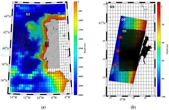
Figure 2.
Study area with the extents of the numerical domains and bathymetry used for SWAN implementations, the downscale of the BCC-CSM1.1 GCM (a) using a nested approach (D1, D2, and D3), and the wave propagation in the hydrodynamic model (b) in the study area (D4 and D5). The red dots indicate the grid nodes assessed in terms of wave parameters to determine the return periods.
Similar to [50,51], the BCC-CSM1.1 GCM wave field was imposed as a time and space varying boundary, with a temporal resolution of 6 h. A wave spectrum of 25 frequencies (0.0418–1 Hz) and 36 directional bands was applied. The model was also forced with 3-hourly winds from the BCC-CSM1.1 GCM r1i1p1 (rip refers to realization, initialization method, and physics version used). The use of a GCM instead of a Regional Climate Model (RCM) is explained by the lack of an RCM using this GCM for this particular region. This GCM is characterized by a horizontal resolution of 1.125° × 1.125° with a 3-hourly temporal resolution. The physical parameters included a stage 1 IEC model and triads, bottom friction, depth-induced breaking, and quadruplets [50,51,66]. The simulations were run for the climate periods between 1979–2005, 2026–2045, and 2081–2099, being the historical, near future, and far future periods. The model validation under wave force was done in previous studies [50,51] for the coastal region (for detailed description, the reader is referred to [50,51]).
The second step was used to simulate the scenarios under different climate periods and return periods. This local model was developed using a nested approach with 2 domains, one covering the coastal region close to the port entrance (D4—Figure 2b) extended from 40.3° N to 41° N and a fringe of 30 km distance to coast, and a horizontal resolution of 1 km. The second domain (D5—Figure 2b) used the same numerical grid and bathymetry used in the FLOW module. SWAN can perform computations on a curvilinear grid, allowing the same grid for FLOW and SWAN, which permits the perfect coupling between the modules.
The model physics was similar to those used for the GCM downscaling purpose, including triads, bottom friction, depth-induced breaking, and whitecapping computed with Komen exponential term [67]. The diffraction and reflections are also available. The wave spectrum was discretized to 25 frequencies (0.0418–1 Hz) and 36 directional bands.
3.3.4. Characterization of Hs, Tp, and Dm
Studying extreme waves on a coastal location was based on analyzing the wave parameters Hs, Tp, and Dm (mean wave direction). These parameters are often used to study the extreme waves, including runup, erosion, and wave-driven longshore transport, which can change the coastal processes during these events [61,68]. Additionally, coastal flooding highly depends on Hs and Tp combined with high tides and storm surges (see Section 2.1) [69].
For this purpose, starting from the downscaled results of the BCC-CSM1.1 GCM, three grid nodes located in front of the port entrance and parallel to the shore were selected as control points (Figure 2b) to calculate the return periods for the wave parameters. The hourly values obtained over 1979–2005 were used to determine the maximum Hs and Tp and fitted to statistical distributions, similar to the approach described in 3.2 for the river discharge and was used to estimate Hs and Tp for Tr10, Tr25, and Tr100.
The Dm is depicted in Figure 3, showing wave arrival predominant from northwest and north-northwest direction for the historical climate during winter, in agreement with previous studies [70,71] for the historic period. Following these results and taking into account [72], the mean wave direction will be the mean of the predominant wave directions. The wave parameters can be seen in Table 6.
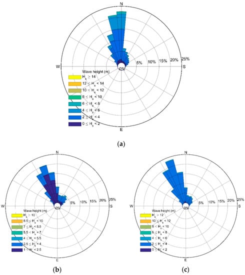
Figure 3.
Mean wave direction for the control points (Figure 2b) for (a) the historical (1979–2005), (b) near future (2026–2045), and (c) far future (2081–2099) periods.
Table 6.
Wave height (Hs), peak period (Tp), and mean wave direction (Dm) for each climate period and return period.
3.4. Hydrodynamic Model
Delft3D suite was used to simulate the study area’s hydrodynamic due to the available features that comprise tide and wind-driven flows, river flow, and wave-driven currents. The hydrodynamic conditions are modeled in the Delft3D-FLOW module [73] and are used in the WAVE module [74], which are executed in a combination between the modules allowing a two-way wave-current interaction.
The Delft3D-FLOW module was used to simulate the flood extent in Aveiro Port. Flow module simulates the two-dimensional (2D) unsteady flow resulting from oceanic, fluvial, and atmospheric drivers. An overview of the model physics can be found in [73]. A 2D model was set up with 577 × 421 cells curvilinear irregular grid with space varying resolution (D5—Figure 2b), where a higher resolution is found in the port jurisdiction area (25 m) (Figure 1b). The bathymetry was constructed based on several sources. In the coastal region, the General Bathymetric Chart of the Oceans (GEBCO)was used, and for the port’s region, multibeam bathymetry data collected in March of 2020 was used [75]. Detailed topographic data was obtained from the Aveiro Port Administration for the marginal areas under the port jurisdiction. Concerning the lagoon channels, bathymetry data from surveys performed between 1987 and 2012 [29] were used, while the topography for the lagoon was obtained from LIDAR topographic data in 2011, provided by the Portuguese General Direction of the Territory. The modeling time step was 60 s, and the bottom roughness was estimated with a standard coefficient of friction [76]. Background horizontal viscosity and diffusivity were set to 10 m2s−1. The model provided outputs with a temporal resolution of 5 min.
The model calibration and validation using the model setup described above was determined for two distinct periods and different open boundaries, aiming at different purposes: the tide propagation (i) and the storm surge (ii).
The model was calibrated and validated for tidal propagation (i) considering the surveys conducted in July of 2019 and between 2002 and 2003 for the stations shown in Figure 1a. To fulfill this task, the model calibration setup was forced at the open boundaries with the astronomic constituents obtained from Oregon State University (OSU) TOPEX/Poseidon Global Inverse Solution 8.0. The calibration simulation was modeled for July of 2019, with one month as spin-up. The calibration process was performed by determining the RMSE and Skill [38] between measured and simulated time series of the sea surface elevation at the stations (Table 7). An RMSE close to zero and a Skill higher than 0.95 represent an excellent agreement between the measured and simulated sea surface elevation [38].
Table 7.
Model performance under tidal propagation resulting from the calibration procedure.
Overall, the model’s ability to predict the spring-neap cycle in the port region (stations BA, SJ, CI, P2) is excellent. The highest disagreements were found in the inner stations showing higher RMSE and lower Skill. These results are in agreement with previous studies [28,38,77], where the best results were found near the lagoon mouth, in the port jurisdiction surroundings, showing RMSEs ranging from 0.06 to 0.08 m in BA, 0.06 to 0.11 m in JS, 0.13 to 0.15 m in CI, and around 0.08 for P2.
The model validation for storm surge forcing (ii) was done for an event identified by [38] that occurred between 19th and 20th January 2013, which was monitored in seven stations located inside the lagoon.
The model setup was forced at the open boundaries using the same approach followed in [38], by prescribing a sea level at the open ocean boundary retrieved from the NEMO-v3.6 model, which comprises a spatial resolution of 0.028° and hourly outputs and is forced by the atmospheric pressure component (http://marine.copernicus.eu, accessed on 27 February 2021). The use of this database relies on the numerical domain limitation in space, as for a good discretization of the surge propagation, a large domain is required. In addition, the model setup was forced with mean sea level pressure and wind components at 10 m retrieved from Meteogalicia (http://mandeo.meteogalicia.es, accessed on 27 February 2021), with a spatial resolution of 12 km and hourly outputs. A spin-up of one month was used similarly to the calibration procedure described in (i).
The validation process was performed comparing the peak values for model results and observations residual levels (Figure 4) and determining the RMSE between these time series (Table 8). The model underestimates the observed surge peak, and the RMSE increases towards the inner lagoon stations, namely for the RN station, where an RMSE of 0.27 m is observed due to the proximity of the largest river discharging in the lagoon and the observed riverine data shortage. The remaining stations show an RMSE under 0.12 m, similar to those found in [38], and therefore the model is considered validated.
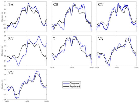
Figure 4.
Residuals for observations (blue line) and model results (black line) under the storm surge event in January 2013.
Table 8.
Model performance under storm surge propagation resulting from the validation procedure.
3.5. Scenarios Design
The scenarios were modeled using the coupling between WAVE and FLOW modules. The hydrodynamic model was run using the ESL, taking into account the relative sea level, storm surge and tide (Section 3.1), the riverine discharges (Section 3.2), and the wave parameters (Section 3.3.3) depicted in Table 6. The hydrodynamic implementation was used to simulate the historical, near, and far future periods for the Tr10, Tr25, and Tr100. A reference scenario representing the present climate extreme level was also determined, taking into account the inputs in Table 1 and Table 2. Table 9 shows an overview of the scenarios determined to assess the flood at Aveiro Port.
Table 9.
Scenario definition. Extreme sea levels (ESL, m) and riverine discharge for Vouga (rd, m3/s) for the 10-, 25-, and 100-year return periods for the reference scenario (referred to present climate), and the historical (1979–2005), near (2026–2045) and far future (2081–2099) periods.
For each scenario, time series of sea levels and river discharges were constructed to impose at the oceanic and land boundaries, respectively. Figure 5 shows these time series for the historical period under the Tr100 as an example, highlighting the moment when the peak of the ESL was obtained. Regarding the oceanic boundary, a similar approach to [25] was conducted, taking into account the sea level evolution and a storm surge event coincident with high tide. For this purpose, the tidal constants of 2019 obtained from the tidal gauge located at the lagoon entrance (Figure 1b) were used to reconstruct the tidal signal in order to determine the tidal range and the level of mean high water springs (for a detailed methodology the reader is referred to [29,30]). The storm surge height was generated synthetically using a sine function and assuming that the storm surge persists for 3 days. The tidal and storm signals were then added, matching the storm surge to the level of mean high water springs (see the orange dashed line in Figure 5). Regarding river discharges, a constant value (annual average) was used in the first 9 days of simulation, rising to the peak value in the last 2 days (see the blue dashed line in Figure 5).
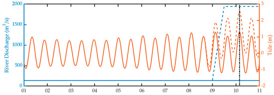
Figure 5.
The historical period under the 100-year return period scenario setup. Continuous lines represent the reference conditions, while the dashed line considers the 100-year return period conditions for riverine discharge and extreme sea level.
Each scenario was run for Tr10: the initial 8 days were used as a spin-up with a tide and discharge considering the reference values. In the following 2 days, an increase of the discharge was imposed, reaching its peak simultaneously with the tide representing the ESL for each climate period and return period. Figure 5 shows the simulation setup for the historical period under the Tr100, highlighting when the peak of the ESL was obtained.
Identifying the driver that contributes most to the Aveiro Port’s inundation was also assessed by a set of simulations considering the far future scenario and Tr100 of ESL, storm surges, waves, and riverine discharges. To fulfill this task, each simulation considered only a single driver independently (e.g., MSLR, without other oceanic drivers during the simulation) and was subsequently compared to the Reference scenario.
4. Results and Discussion
The flood assessment of Aveiro Port was carried out for the historical, near and far future periods, considering the flood drivers for Tr10, Tr25, and Tr100. Flood extent maps and flooded areas of the Aveiro Port’s terminals and zones under its jurisdiction for the historical, near, and far future scenarios and for each return period were determined. The flood assessment is conducted considering the reference level as a starting point, where no flood is present for the entire port jurisdiction area. This scenario considers the tide with the historical MSL and average riverine discharges. A comparison between the reference and the Tr10, Tr25, and Tr100 of ESL, storm surges, waves, and riverine discharge scenarios is conducted, indicating the port terminals susceptible to floods and the corresponding flooded area (Table 10).
Table 10.
Flooded areas of the terminals (Figure 1) at the Aveiro Port shown in percentage (%) relative to the total area of each terminal for the historical (H), near (NF), and far future (FF) periods and for the 10-, 25-, and 100-year return periods. Terminal 10 is not shown due to being designed as a single berthing dock.
Concerning the historical period (1979–2005) (Figure 6a), the flooded areas are located primarily on the central lagoon region for a Tr10 and increase with the return period. Although this region is in the port’s jurisdiction, it is not relevant since it is not used for port activities. However, some floods can occur in the Shipping Repair/Construction Zone (7), Services, Logistics Zone (8) (Figure 6b), and in the Small Harbor (12), showing around 68.1, 49.3, and 61.8% for Tr10, respectively, and leading partially to complete inundation under the Tr100 (76.5, 77.1 and 98.3%, respectively). Also, even with a Tr10, some marginal areas are inundated for most of the terminals, which are slightly expanded under higher return periods, including most of the terminals and zones covered by the port’s jurisdiction, namely the Liquid Bulk terminal (5), High Sea Fishing (9) and the Offshore Fishing (11) ports, with over 30% of the areas flooded. However, the Multipurpose South Terminal (6) shows a complete inundation under all climate scenarios for the Tr10, Tr25, and Tr100. The flood extent shown under the historical period shows that Aveiro Port’s resilience to floods is high under Tr10 and Tr25, showing some vulnerable areas under the Tr100 scenario.
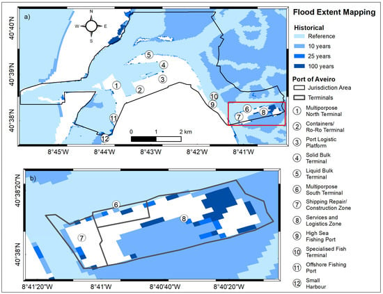
Figure 6.
Flood extent mapping of the Aveiro Port’s terminals and zones (numbers 1–12) under its jurisdiction (a) (black line) and zoom of the most flooded area (b) (red line). Reference scenario under present climate and 10-, 25-, and 100-year return period are determined for the historical (1979–2005) climate period.
In contrast to the historical period, the upcoming climate represented by the near-future period (2026–2045) (Figure 7a) shows a significant flood extent. The port’s terminal area affected by flood increased under Tr10, being more prominent in the Offshore Fishing (11) and Small Harbor (12) (a rise of 7 and 24.6% from the historical period, respectively). The Small Harbor (12) is almost totally flooded under the depicted scenarios and will keep this trend for the far future period scenarios. The flood rate is more evident under Tr25 and Tr100, where most of the zones 5, 9, and 12 are near to completely flooded in contrast with the previous climate scenario. Most of the terminals and zones show marginal flood, where the Port Logistic Platform (3) shows a sizeable marginal flood under Tr100. The most vulnerable port areas under the historical period (Figure 7b) worsened under this climate scenario, where over three-quarters of these terminals are flooded.
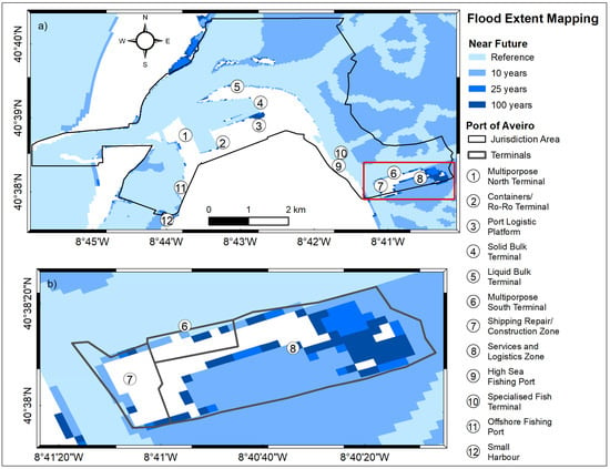
Figure 7.
Flood extent mapping of the Aveiro Port’s terminals and zones (numbers 1–12) under its jurisdiction (a) (black line) and zoom of the most flooded area (b) (red line). Reference scenario under present climate and 10-, 25-, and 100-year return period are determined for the near future (2026–2045) climate period.
Previous works demonstrated that climate change is expected to increase Ria de Aveiro’s flood hazard [30] due to increased oceanic and fluvial drivers, posing higher impacts at the end of the century [24]. In this context, and analyzing the flood extent maps under far future climate drivers (Figure 8a), the marginal areas of most significant risk for Tr10 are all terminals and zones under Aveiro Port’s jurisdiction as well as the Services and Logistics Zone (8), where the highest flood area increase was observed (12.3%) from the previous climate scenario. For the Tr25 the inundation extent increases, and Shipping Repair/Construction (7) and Services and Logistics (8) Zones are at risk of being completely flooded. The Containers/Ro-Ro Terminal (2) and Port Logistic Platform (3) will be subject to significant inundation, being both considerably affected by the far future meteocean drivers.
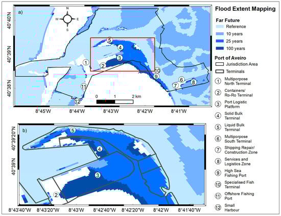
Figure 8.
Flood extent mapping of the Aveiro Port’s terminals and zones (numbers 1–12) under its jurisdiction (a) (black line) and zoom of the most flooded area (b) (red line). Reference scenario under present climate and 10-, 25-, and 100-year return period are determined for the far future (2081–2099) climate period.
Regarding the Tr100, the flood extent increases significantly at most terminals, covering higher areas than for the Tr25. The Services and Logistics Zone (8) is almost completely flooded, similarly to the High Sea Fishing Port (9) and Liquid Bulk Terminal (5), where most of the areas will be inundated. With the mean sea-level rise under this scenario, the flooded area now comprises a large section of the Port Logistic Platform (3) and the Offshore Fishing Port (11), and marginal flooding of the Solid Bulk Terminal (4). Analyzing the entire port jurisdiction area, only the Multipurpose North Terminal (1) and the Contentainers/Ro-Ro Terminal (2) suffer a small marginal inundation, indicating a low risk of flooding.
Evaluating the overall evolution of the flood extent during the different climatic scenarios studied, the severity of the flood extent is noticeable over the port’s jurisdiction area, although some areas are more vulnerable to climate change than others. These areas could be impacted differently compared to the climate change drivers taken into consideration for this study. Therefore, the contribution that these make to flood extent in Aveiro Port requires further investigation. Thus, a set of simulations were run considering the far future scenario and Tr100 of ESL, storm surges, waves, and riverine discharges in order to identify the driver that contributes most to the Aveiro Port’s inundation (Figure 9).
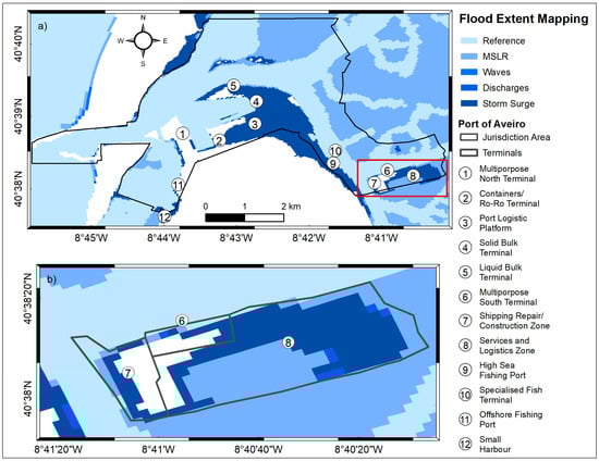
Figure 9.
Flood extent mapping of the Aveiro Port’s terminals and zones (numbers 1–12) under its jurisdiction (a) (black line) and zoom of the most flooded area (b) (red line). Reference scenario and 100-year return period drivers for the far future (2081–2099) climate period, considering the climate drivers individually.
The MSLR is an important driver primarily due to the contribution to the total water level and can worsen when other oceanic drivers occur. In a scenario where the MSLR is the only driver, the Aveiro Port’s area affected by the flood comprises its jurisdiction area’s central region, mainly affecting the marginal region of all the terminals and zones. An exception is observed at the Services and Logistics Zone (8), where the inundation occurs in most areas (Figure 9b). This inundation area increases when high riverine discharges occur, mainly in the Services and Logistics Zone (8) due to its proximity to the Vouga river, the most important contributor in terms of flow to the lagoon. On the other hand, the waves driver is residual, which is expected to lagoon geometry and natural protection from the sea waves. The most prevalent oceanic driver is the storm surge, whose flood area comprises most of the total inundation of most terminals, and the flood extent is highly correlated to the same extent shown in Figure 8.
The definition of adaptation or mitigation countermeasures against flooding is not straightforward due to the high uncertainty of projections related to climate change’s multiple spatial and time scales. Climate projections rely on probabilities of occurring specific processes, and ports tend to focus on general conditions that they observed and act accordingly by adapting or building new structures to reduce the impacts. The port’s planning horizons are also around 5 to 10 years [78] and are subject to the volatility of the changing business circumstances. These time scales are much shorter than existing infrastructures and typical climate change time scales, which are on the scale of 30 to hundreds of years, making it challenging to implement efficient long-term measures.
Moreover, there is a geographic scale mismatch between the Aveiro Lagoon and the Aveiro Port jurisdiction. While Aveiro Port can act on its jurisdiction area, some planning could occur outside of this area, involving third-party private or business stakeholders.
Drawing on the above, planning responses could be acted on the resilience of the infrastructures and operational measures, like relocating the terminals and zones according to the commercial and value of the goods.
5. Conclusions
The present study assesses the flooding extension on Aveiro Port in a climate change context under the RCP8.5 scenario, providing an overview of the key areas impacted by the floods in Aveiro Port. Towards this objective, spatial flood extent maps were generated for the Aveiro Port jurisdiction area to assess and quantify the impact of climate change drivers for 10-, 25-, and 100-year return period scenarios, identifying the port terminals susceptible to flood under each scenario. The climate drivers were also assessed to identify the most prevailing driver to the inundation of the Aveiro Port.
Aveiro Port, the most recent port in Portugal, is located in a low-lying lagoon, and the planned longevity of the infrastructure assets and port is inherently exposed to climate change drivers, such as rising MSL and ESL and riverine floods. As a result of these risks, Aveiro Port faces floods in the current climate, which can worsen drastically at the end of the century, if climate change drivers continue to accelerate as predicted, leading to large floods.
The results of this study also highlighted the flood extension impact of the drivers under climate change scenarios, which is quite pronounced for all the return period scenarios at the end of the century on most of the terminals and zones. Some of the port areas will be profoundly affected, namely within the innermost jurisdiction area where the riverine discharges and storm surges, along with MLSR, contribute the most to the inundation pattern, which may lead to possible disruptions in operations and damages on property, resulting in serious economic repercussions due to Aveiro Port value to the region. Similar impacts of extensive floods due to the worsening of the climate drivers are expected in most of the ports located on the Atlantic coast of Europe [24,25].
Aveiro Port’s vulnerability to rising sea levels will require planning adaptation measures to increase the port’s resilience to climate change. Such measures to deal with long-term prospects of high flood extents must be assessed by forecasting the flood areas and identifying vulnerable locations since most of the infrastructures lie in seas areas threatened by the relative sea-level rise.
In summary, this study provides a valuable methodology to analyze the projected flooding extent on Aveiro Port under extreme climate change scenarios and, therefore, can be replicated and applied to other ports at risk due to climate change. Therefore, the flood assessment must be considered a support toolkit to identify the port’s weakness to assist in the definition of adaptation, management, and resilience measures for future challenges.
Author Contributions
Conceptualization, A.S.R., C.L.L. and J.M.D.; methodology, A.S.R., C.L.L. and M.G.-G.; software, A.S.R., C.L.L., M.C.S. and M.G.-G.; validation, M.C.S., M.G.-G. and J.M.D.; investigation, A.S.R. and C.L.L.; writing—original draft preparation, A.S.R.; writing—review and editing, A.S.R., C.L.L., M.C.S., M.G.-G. and J.M.D.; visualization, M.C.S., M.G.-G. and J.M.D.; supervision, J.M.D. and M.G.-G.; funding acquisition, J.M.D. and M.G.-G. All authors have read and agreed to the published version of the manuscript.
Funding
The first author of this work has been supported by the Portuguese Science Foundation (FCT) through a doctoral grant (SFRH/BD/114919/2016). The second author is funded by national funds through the Portuguese Science Foundation (FCT) under the project CEECIND/00459/2018. The third author is funded by national funds (OE), through FCT, I.P., in the scope of the framework contract foreseen in the numbers 4, 5, and 6 of the article 23, of the Decree-Law 57/2016, of August 29, changed by Law 57/2017, of July 19. Thanks are due to FCT/MCTES for the financial support to CESAM (UIDB/50017/2020+UIDP/50017/2020) through national funds. The present study is also part of the project “WECAnet: A pan-European network for Marine Renewable Energy” (CA17105), which received funding from the HORIZON2020 Framework Program by COST (European Cooperation in Science and Technology), a funding agency for research and innovation networks.
Institutional Review Board Statement
Not applicable.
Informed Consent Statement
Not applicable.
Data Availability Statement
Data available on request due to funding restrictions. The data presented in this study are available on request from the corresponding author. The data are not publicly available due to funding restrictions.
Acknowledgments
The authors acknowledge the regional sea level data from IPCC AR5 distributed in netCDF format by the Integrated Climate Data Center (ICDC, icdc.cen.uni-hamburg.de) University of Hamburg, Hamburg, Germany. The authors also acknowledge the topography data provided by the Aveiro Port Administration, Aveiro, Portugal.
Conflicts of Interest
The authors declare no conflict of interest. The funders had no role in the design of the study; in the collection, analyses, or interpretation of data; in the writing of the manuscript, or in the decision to publish the results.
References
- United Nations. Review of Maritime Transport 2019 (UNCTAD/RMT/2019); United Nations Conference on Trade and Development, Ed.; United Nations: New York, NY, USA, 2019; ISBN 978-92-1-112958-8. [Google Scholar]
- United Nations. TRADE AND DEVELOPMENT Report 2020 (UNCTAD/TDR/2020); United Nations Conference on Trade and Development, Ed.; United Nations: New York, NY, USA, 2020; ISBN 978-92-1-112992-2. [Google Scholar]
- Rodrigue, J.-P.; Comtois, C.; Slack, B. The Geography of Transport Systems, 4th ed.; Routledge: London, UK, 2016; ISBN 9781315618159. [Google Scholar]
- Le Carrer, N.; Ferson, S.; Green, P.L. Optimising cargo loading and ship scheduling in tidal areas. Eur. J. Oper. Res. 2020, 280, 1082–1094. [Google Scholar] [CrossRef]
- Song, J.-H.; Furman, K.C. A maritime inventory routing problem: Practical approach. Comput. Oper. Res. 2013, 40, 657–665. [Google Scholar] [CrossRef]
- Kirezci, E.; Young, I.R.; Ranasinghe, R.; Muis, S.; Nicholls, R.J.; Lincke, D.; Hinkel, J. Projections of global-scale extreme sea levels and resulting episodic coastal flooding over the 21st Century. Sci. Rep. 2020, 10, 11629. [Google Scholar] [CrossRef] [PubMed]
- Kusunoki, S.; Ose, T.; Hosaka, M. Emergence of unprecedented climate change in projected future precipitation. Sci. Rep. 2020, 10, 4802. [Google Scholar] [CrossRef]
- Reguero, B.G.; Losada, I.J.; Méndez, F.J. A recent increase in global wave power as a consequence of oceanic warming. Nat. Commun. 2019. [Google Scholar] [CrossRef]
- Hawkins, E.; Frame, D.; Harrington, L.; Joshi, M.; King, A.; Rojas, M.; Sutton, R. Observed Emergence of the Climate Change Signal: From the Familiar to the Unknown. Geophys. Res. Lett. 2020, 47. [Google Scholar] [CrossRef]
- Kulp, S.A.; Strauss, B.H. New elevation data triple estimates of global vulnerability to sea-level rise and coastal flooding. Nat. Commun. 2019, 10, 4844. [Google Scholar] [CrossRef]
- Jackson, L.P.; Jevrejeva, S. A probabilistic approach to 21st century regional sea-level projections using RCP and High-end scenarios. Glob. Planet. Chang. 2016, 146, 179–189. [Google Scholar] [CrossRef]
- IPCC. Climate Change 2014: Synthesis Report. Contribution of Working Groups I, II and III to the Fifth Assessment Report of the Intergovernmental Panel on Climate Change; Core Writing Team, Pachauri, R.K., Meyer, L.A., Eds.; The Intergovernmental Panel on Climate Change: Geneva, Switzerland, 2014; ISBN 9789291691432. [Google Scholar]
- Santamaría-Gómez, A.; Gravelle, M.; Dangendorf, S.; Marcos, M.; Spada, G.; Wöppelmann, G. Uncertainty of the 20th century sea-level rise due to vertical land motion errors. Earth Planet. Sci. Lett. 2017, 473, 24–32. [Google Scholar] [CrossRef]
- Bonaduce, A.; Pinardi, N.; Oddo, P.; Spada, G.; Larnicol, G. Sea-level variability in the Mediterranean Sea from altimetry and tide gauges. Clim. Dyn. 2016, 47, 2851–2866. [Google Scholar] [CrossRef]
- Vousdoukas, M.I.; Voukouvalas, E.; Annunziato, A.; Giardino, A.; Feyen, L. Projections of extreme storm surge levels along Europe. Clim. Dyn. 2016, 47, 3171–3190. [Google Scholar] [CrossRef]
- Harrison, G.P.; Wallace, A.R. Sensitivity of Wave Energy to Climate Change. IEEE Trans. Energy Convers. 2005, 20, 870–877. [Google Scholar] [CrossRef]
- Swain, D.L.; Singh, D.; Touma, D.; Diffenbaugh, N.S. Attributing Extreme Events to Climate Change: A New Frontier in a Warming World. One Earth 2020, 2, 522–527. [Google Scholar] [CrossRef]
- Diffenbaugh, N.S.; Singh, D.; Mankin, J.S.; Horton, D.E.; Swain, D.L.; Touma, D.; Charland, A.; Liu, Y.; Haugen, M.; Tsiang, M.; et al. Quantifying the influence of global warming on unprecedented extreme climate events. Proc. Natl. Acad. Sci. USA 2017, 114, 4881–4886. [Google Scholar] [CrossRef] [PubMed]
- Moemken, J.; Reyers, M.; Feldmann, H.; Pinto, J.G. Future Changes of Wind Speed and Wind Energy Potentials in EURO-CORDEX Ensemble Simulations. J. Geophys. Res. Atmos. 2018, 123, 6373–6389. [Google Scholar] [CrossRef]
- Morim, J.; Trenham, C.; Hemer, M.; Wang, X.L.; Mori, N.; Casas-Prat, M.; Semedo, A.; Shimura, T.; Timmermans, B.; Camus, P.; et al. A global ensemble of ocean wave climate projections from CMIP5-driven models. Sci. Data 2020, 7, 105. [Google Scholar] [CrossRef]
- European Commission COM(2020) 80 Final. Proposal for a Regulation of the European Parliament and of the Council Establishing the Framework for Achieving Climate Neutrality and Amending Regulation (EU) 2018/1999 (European Climate Law); European Commission: Brussels, Belgium, 2020. [Google Scholar]
- European Commission Energy, Climate Change, Environment. Available online: https://ec.europa.eu/info/energy-climate-change-environment_en (accessed on 27 February 2021).
- European Commission EUROSTAT. Available online: https://ec.europa.eu/eurostat/web/main (accessed on 27 February 2021).
- Christodoulou, A.; Christidis, P.; Demirel, H. Sea-level rise in ports: A wider focus on impacts. Marit. Econ. Logist. 2019, 21, 482–496. [Google Scholar] [CrossRef]
- Christodoulou, A.; Demirel, H. Impacts of Climate Change on Transport: A Focus on Airports, Seaports and Inland Waterways; EUR 28896 EN, JRC108865; Publications Office of the European Union: Luxembourg, 2018; ISBN 978-92-79-97039-9. [Google Scholar] [CrossRef]
- da Cruz, M.R.P.; de Matos Ferreira, J.J. Evaluating Iberian seaport competitiveness using an alternative DEA approach. Eur. Transp. Res. Rev. 2016, 8, 1. [Google Scholar] [CrossRef]
- Fortunato, A.B.; Rodrigues, M.; Dias, J.M.; Lopes, C.; Oliveira, A. Generating inundation maps for a coastal lagoon: A case study in the Ria de Aveiro (Portugal). Ocean. Eng. 2013, 64, 60–71. [Google Scholar] [CrossRef]
- Lopes, C.L.; Azevedo, A.; Dias, J.M. Flooding assessment under sea level rise scenarios: Ria de Aveiro case study. J. Coast. Res. 2013, 65, 766–771. [Google Scholar] [CrossRef]
- Lopes, C.L.; Dias, J.M. Assessment of flood hazard during extreme sea levels in a tidally dominated lagoon. Nat. Hazards 2015, 77, 1345–1364. [Google Scholar] [CrossRef]
- Lopes, C.L.; Alves, F.L.; Dias, J.M. Flood risk assessment in a coastal lagoon under present and future scenarios: Ria de Aveiro case study. Nat. Hazards 2017, 89, 1307–1325. [Google Scholar] [CrossRef]
- Moreira, M.H.; Queiroga, H.; Machado, M.M.; Cunha, M.R. Environmental gradients in a southern Europe estuarine system: Ria de Aveiro, Portugal implications for soft bottom macrofauna colonization. Neth. J. Aquat. Ecol. 1993, 27, 465–482. [Google Scholar] [CrossRef]
- Dias, J.M.; Lopes, J.F.; Dekeyser, I. Tidal propagation in Ria de Aveiro Lagoon, Portugal. Phys. Chem. Earth Part B Hydrol. Ocean. Atmos. 2000, 25, 369–374. [Google Scholar] [CrossRef]
- Vaz, N.; Miguel Dias, J.; Chambel Leitão, P. Three-dimensional modelling of a tidal channel: The Espinheiro Channel (Portugal). Cont. Shelf Res. 2009, 29, 29–41. [Google Scholar] [CrossRef]
- Pereira, C.; Coelho, C. Mapping erosion risk under different scenarios of climate change for Aveiro coast, Portugal. Nat. Hazards 2013, 69, 1033–1050. [Google Scholar] [CrossRef]
- Lopes, C.L.; Silva, P.A.; Dias, J.M.; Rocha, A.; Picado, A.; Plecha, S.; Fortunato, A.B. Local sea level change scenarios for the end of the 21st century and potential physical impacts in the lower Ria de Aveiro (Portugal). Cont. Shelf Res. 2011, 31, 1515–1526. [Google Scholar] [CrossRef]
- Plecha, S.; Silva, P.A.; Vaz, N.; Bertin, X.; Oliveira, A.; Fortunato, A.B.; Dias, J.M. Sensitivity analysis of a morphodynamic modelling system applied to a coastal lagoon inlet. Ocean. Dyn. 2010, 60, 275–284. [Google Scholar] [CrossRef]
- Picado, A.; Lopes, C.L.; Mendes, R.; Vaz, N.; Dias, J.M. Storm surge impact in the hydrodynamics of a tidal lagoon: The case of Ria de Aveiro. J. Coast. Res. 2013, 65, 796–801. [Google Scholar] [CrossRef]
- Pinheiro, J.P.; Lopes, C.L.; Ribeiro, A.S.; Sousa, M.C.; Dias, J.M. Tide-surge interaction in Ria de Aveiro lagoon and its influence in local inundation patterns. Cont. Shelf Res. 2020, 200, 104132. [Google Scholar] [CrossRef]
- Lopes, C.L.; Plecha, S.; Silva, P.A.; Dias, J.M. Influence of morphological changes in a lagoon flooding extension: Case study of Ria de Aveiro (Portugal). J. Coast. Res. 2013, 165, 1158–1163. [Google Scholar] [CrossRef]
- Fidélis, T.; Teles, F.; Roebeling, P.; Riazi, F. Governance for Sustainability of Estuarine Areas—Assessing Alternative Models Using the Case of Ria de Aveiro, Portugal. Water 2019, 11, 846. [Google Scholar] [CrossRef]
- Pedersen, J.S.T.; van Vuuren, D.P.; Aparício, B.A.; Swart, R.; Gupta, J.; Santos, F.D. Variability in historical emissions trends suggests a need for a wide range of global scenarios and regional analyses. Commun. Earth Environ. 2020, 1, 41. [Google Scholar] [CrossRef]
- Woodworth, P.L. A survey of recent changes in the main components of the ocean tide. Cont. Shelf Res. 2010, 30, 1680–1691. [Google Scholar] [CrossRef]
- Garner, A.J.; Mann, M.E.; Emanuel, K.A.; Kopp, R.E.; Lin, N.; Alley, R.B.; Horton, B.P.; DeConto, R.M.; Donnelly, J.P.; Pollard, D. Impact of climate change on New York City’s coastal flood hazard: Increasing flood heights from the preindustrial to 2300 CE. Proc. Natl. Acad. Sci. USA 2017, 114, 11861–11866. [Google Scholar] [CrossRef] [PubMed]
- Rahmstorf, S. Rising hazard of storm-surge flooding. Proc. Natl. Acad. Sci. USA 2017, 114, 11806–11808. [Google Scholar] [CrossRef] [PubMed]
- Arnold, J.G.; Allen, P.M.; Bernhardt, G. A comprehensive surface-groundwater flow model. J. Hydrol. 1993, 142, 47–69. [Google Scholar] [CrossRef]
- Dias, J.M.; Alves, F.L.; Coelho, C.; Rocha, A.; Fortunato, A.B.; Lopes, C.L.; Sousa, L.; Pereira, C.; Rodrigues, N.T.R.; Silva, P.A.; et al. ADAPTARia: Modelação das Alterações Climáticas no Litoral da Ria de Aveiro—Estratégias de Adaptação para Cheias Costeiras e Fluviais; National Laboratory for Civil Engineering: Aveiro, Portugal, 2013. [Google Scholar]
- Sousa, M.C.; Ribeiro, A.; Des, M.; Gomez-Gesteira, M.; deCastro, M.; Dias, J.M. NW Iberian Peninsula coastal upwelling future weakening: Competition between wind intensification and surface heating. Sci. Total Environ. 2020, 703, 134808. [Google Scholar] [CrossRef] [PubMed]
- Durrant, T.; Hemer, M.; Smith, G.; Trenham, C.; Greenslade, D. CAWCR Wave Hindcast—Aggregated Collection; CSIRO. Service Collection: Canberra, Australia, 2019; Volume 5. [CrossRef]
- Hemer, M.; Trenham, C.; Durant, T.; Greenslade, D. CAWCR Global Wind-Wave 21st Century Climate Projections; CSIRO. Service Collection: Canberra, Australia, 2015; Volume 2.
- Ribeiro, A.S.; DeCastro, M.; Rusu, L.; Bernardino, M.; Dias, J.M.; Gomez-Gesteira, M. Evaluating the Future Efficiency of Wave Energy Converters along the NW Coast of the Iberian Peninsula. Energies 2020, 13, 3563. [Google Scholar] [CrossRef]
- Ribeiro, A.; Costoya, X.; de Castro, M.; Carvalho, D.; Dias, J.M.; Rocha, A.; Gomez-Gesteira, M. Assessment of Hybrid Wind-Wave Energy Resource for the NW Coast of Iberian Peninsula in a Climate Change Context. Appl. Sci. 2020, 10, 7395. [Google Scholar] [CrossRef]
- Fu, G.; Liu, Z.; Charles, S.P.; Xu, Z.; Yao, Z. A score-based method for assessing the performance of GCMs: A case study of southeastern Australia. J. Geophys. Res. Atmos. 2013, 118, 4154–4167. [Google Scholar] [CrossRef]
- Perkins, S.E.; Pitman, A.J.; Holbrook, N.J.; McAneney, J. Evaluation of the AR4 climate models’ simulated daily maximum temperature, minimum temperature, and precipitation over Australia using probability density functions. J. Clim. 2007, 20, 4356–4376. [Google Scholar] [CrossRef]
- Perkins, S.E.; Pitman, A.J.; Sisson, S.A. Smaller projected increases in 20-year temperature returns over Australia in skill-selected climate models. Geophys. Res. Lett. 2009, 36, L06710. [Google Scholar] [CrossRef]
- Perkins, S.E.; Pitman, A.J.; Sisson, S.A. Systematic differences in future 20 year temperature extremes in AR4 model projections over Australia as a function of model skill. Int. J. Climatol. 2013, 33, 1153–1167. [Google Scholar] [CrossRef]
- Sun, Q.; Miao, C.; Duan, Q. Comparative analysis of CMIP3 and CMIP5 global climate models for simulating the daily mean, maximum, and minimum temperatures and daily precipitation over China. J. Geophys. Res. Atmos. 2015, 120, 4806–4824. [Google Scholar] [CrossRef]
- Maxino, C.C.; McAvaney, B.J.; Pitman, A.J.; Perkins, S.E. Ranking the AR4 climate models over the Murray-Darling Basin using simulated maximum temperature, minimum temperature and precipitation. Int. J. Climatol. 2008, 28, 1097–1112. [Google Scholar] [CrossRef]
- Errasti, I.; Ezcurra, A.; Sáenz, J.; Ibarra-Berastegi, G. Validation of IPCC AR4 models over the Iberian Peninsula. Theor. Appl. Climatol. 2011, 103, 61–79. [Google Scholar] [CrossRef]
- Krishnan, A.; Bhaskaran, P.K. Skill assessment of global climate model wind speed from CMIP5 and CMIP6 and evaluation of projections for the Bay of Bengal. Clim. Dyn. 2020, 55, 2667–2687. [Google Scholar] [CrossRef]
- Hemer, M.A.; Trenham, C.E. Evaluation of a CMIP5 derived dynamical global wind wave climate model ensemble. Ocean. Model. 2016, 103, 190–203. [Google Scholar] [CrossRef]
- Erikson, L.H.; Hegermiller, C.A.; Barnard, P.L.; Ruggiero, P.; van Ormondt, M. Projected wave conditions in the Eastern North Pacific under the influence of two CMIP5 climate scenarios. Ocean. Model. 2015, 96, 171–185. [Google Scholar] [CrossRef]
- Camus, P.; Losada, I.J.; Izaguirre, C.; Espejo, A.; Menéndez, M.; Pérez, J. Statistical wave climate projections for coastal impact assessments. Earth Futur. 2017, 5, 918–933. [Google Scholar] [CrossRef]
- Shimura, T.; Mori, N.; Hemer, M.A. Variability and future decreases in winter wave heights in the Western North Pacific. Geophys. Res. Lett. 2016, 43, 2716–2722. [Google Scholar] [CrossRef]
- Izaguirre, C.; Mendez, F.J.; Menendez, M.; Luceño, A.; Losada, I.J. Extreme wave climate variability in southern Europe using satellite data. J. Geophys. Res. 2010, 115, C04009. [Google Scholar] [CrossRef]
- SWAN. SWAN User Manual Version 41.31; Delft University of Technology, Environmental Fluid Mechanics Section: Delft, The Netherlands, 2019; Volume 143. [Google Scholar]
- IEC TS 62600-101. Marine Energy—Wave, Tidal and Other Water Current Converters—Part 100: Electricity Producing Wave Energy Converters—Power Performance Assessment; International Electrotechnical Commission: Geneva, Switzerland, 2015; ISBN 9782832227244. [Google Scholar]
- Komen, G.J.; Hasselmann, K.; Hasselmann, K. On the Existence of a Fully Developed Wind-Sea Spectrum. J. Phys. Oceanogr. 1984, 14, 1271–1285. [Google Scholar] [CrossRef]
- Splinter, K.D.; Davidson, M.A.; Golshani, A.; Tomlinson, R. Climate controls on longshore sediment transport. Cont. Shelf Res. 2012, 48, 146–156. [Google Scholar] [CrossRef]
- Bromirski, P.D.; Cayan, D.R.; Helly, J.; Wittmann, P. Wave power variability and trends across the North Pacific. J. Geophys. Res. Ocean. 2013, 118, 6329–6348. [Google Scholar] [CrossRef]
- Silva, D.; Bento, A.R.; Martinho, P.; Guedes Soares, C. High resolution local wave energy modelling in the Iberian Peninsula. Energy 2015, 91, 1099–1112. [Google Scholar] [CrossRef]
- Oliveira, T.C.A.; Cagnin, E.; Silva, P.A. Wind-waves in the coast of mainland Portugal induced by post-tropical storms. Ocean. Eng. 2020, 217, 108020. [Google Scholar] [CrossRef]
- World Meteorological Organization. Guide to Wave Analysis and Forecasting, 3rd ed.; World Meteorological Organization (WMO): Geneve, Switzerland, 2018; ISBN 978-92-63-10702-2. [Google Scholar]
- Deltares. Delft3D-FLOW. Simulation of Multi-Dimensional Hydrodynamic Flows and Transport Phenomena, Including Sediments; Version: 3.15 User Manual; Deltares: Delft, The Netherlands, 2020. [Google Scholar]
- Deltares. Delft3D-WAVE. Simulation of Short-Crested Waves with SWAN; Version: 3.05 User Manual; Deltares: Delft, The Netherlands, 2020. [Google Scholar]
- Cavalinhos, R.; Correia, R.; Rosa, P.; Lillebo, A.I.; Pinheiro, L.M. Processed Multibeam Bathymetry Data Collected Around the Ria de Aveiro, Portugal, Onboard the NEREIDE Research Vessel; Zenodo: Meyrin, Switzerland, 2020. [Google Scholar] [CrossRef]
- van Rijn, L.C. Unified View of Sediment Transport by Currents and Waves. I: Initiation of Motion, Bed Roughness, and Bed-Load Transport. J. Hydraul. Eng. 2007, 133, 649–667. [Google Scholar] [CrossRef]
- Vargas, C.I.C.; Vaz, N.; Dias, J.M. An evaluation of climate change effects in estuarine salinity patterns: Application to Ria de Aveiro shallow water system. Estuar. Coast. Shelf Sci. 2017, 189, 33–45. [Google Scholar] [CrossRef]
- Transportation Research Board and National Research Council. Potential Impacts of Climate Change on U.S. Transportation: Special Report 290; Transportation Research Board: Washington, DC, USA, 2008; ISBN 978-0-309-11306-9. [Google Scholar]


Publisher’s Note: MDPI stays neutral with regard to jurisdictional claims in published maps and institutional affiliations. |
© 2021 by the authors. Licensee MDPI, Basel, Switzerland. This article is an open access article distributed under the terms and conditions of the Creative Commons Attribution (CC BY) license (https://creativecommons.org/licenses/by/4.0/).