Numerical Study of the Pulsation Process of Spark Bubbles under Three Boundary Conditions

Abstract

In this study, a compressible three-phase homogeneous model was established using ABAQUS/Explicit. These models can numerically simulate the pulsation process of cavitation bubbles in the free field, near the flat plate target, and near the curved boundary target. At the same time, these models can numerically simulate the strong nonlinear interaction between the cavitation bubble and its nearby wall boundaries. The mutual flow of liquid and gas and fluid solid coupling were solved by the Euler domain in simulation. The results of the numerical simulation were verified by comparing them with the experimental results. In this study, we used electric spark bubbles to represent cavitation bubbles. A high-speed camera was used to record the pulsation process of cavitation bubbles. This study first verified the pulsation process of cavitation bubbles in the free field, because it was the simplest case. Then we verified the interaction process between cavitation bubbles and different wall boundaries. In order to further confirm the credibility of the numerical simulation results, for each wall surface, this study used two burst distances (10 mm and 25 mm) for simulation verification. The numerical model established in this study could effectively simulate the pulsation characteristics of cavitation bubbles, such as the formation of jets and annular bubbles. After verification, the simulated cavitation bubble was almost the same as the cavitation bubble captured by the high-speed camera in the experiment in terms of time, volume, and shape. In this study, a detailed velocity field of the cavitation bubble collapse stage was obtained, which laid down the foundation for the study of the strong nonlinear interaction between the cavitation bubble and the target plates of different shapes. Compared with the experimental results, we found that the numerical model established by the simulation could accurately simulate the bubble pulsation and jet formation processes. In the experiment, the interval time for the bubble pictures taken by the high-speed camera was 41.66 μs per frame. Using a numerical model, the bubble pulsation process can be simulated at an interval of 1 µs per frame. Therefore, the numerical model established by the simulation could show the movement characteristics of the cavitation bubble pulsation process in more detail.

1. Introduction

Cavitation bubbles are widespread in nature. Moreover, the pressure load generated by the pulsation process of cavitation bubbles can be very destructive. It can severely damage nearby structures. Studying the pulsation process of cavitation bubbles is helpful for the anti-riot prediction and design of ships and marine structures. Therefore, scholars have shown great interest in the study of cavitation bubbles; they call it the dynamics of cavitation bubbles. At present, cavitation bubble dynamics have been widely used in military, medical and engineering disciplines [1].

The pulsation conditions of cavitation bubbles are generally divided into two cases: those with wall boundaries near the cavitation bubbles and those without wall boundaries. When the cavitation bubble pulsates near a borderless wall, it is also called a pulsation in the free field of the cavitation bubble. At this time, the dynamics of cavitation bubbles are relatively simple, so we only need to consider gravity, buoyancy, and the relatively uniform water pressure around the bubbles. Since the cavitation bubbles are far from the water surface and other wall surfaces, they form spherical bubbles during the expansion stage. In the collapse stage, a high-speed water jet is formed, and when the jet passes through the end of the bubble, an annular bubble is formed. At the same time, the bubbles will get closer and closer to the water surface under the action of buoyancy [2], as shown in Figure 1. When there is a wall boundary near the cavitation bubble, the pulsation process is relatively complicated. At this time, the cavitation bubble will interact with the boundary wall, which will have a certain impact on the bubble pulsation process [3]. In addition, the nonlinear interaction between the cavitation bubble and the boundary wall is also affected by the explosion distance, liquid density and boundary shape [4,5,6,7,8,9,10,11]. That is to say, the nonlinear interaction between cavitation bubbles and other structures is a complex three-phase problem involving compressibility effects [12] such as cavitation bubble deformation, shock wave propagation, and cavitation phase change. As well as the heat transfer, boiling and condensation can be caused by changes in ambient temperature, etc. [13,14,15,16,17,18,19].

Therefore, understanding the pulsation process of cavitation bubbles and their interaction with nearby structures during the pulsation process is very important for increasing the vitality of ships and marine structures. In recent years, scholars have conducted extensive experimental and numerical studies on the dynamics of cavitation bubbles.

In terms of experimental research, Liddiard et al. [20] used explosives to obtain underwater explosion bubbles. However, the cavitation bubbles produced by the explosion were affected by many unpredictable factors. The repeatability was not sufficient; for example, shrapnel has an impact on cavitation bubbles after an explosion. Electric spark bubbles have the advantages of good repeatability and stability; therefore, in recent years, scholars have used electric spark technology to produce cavitation bubbles [21]. Compared with explosives, this technology could produce relatively stable and reproducible cavitation bubbles. Gibson and Blake [22] used electric spark technology to study the movement of cavitation bubbles near the flexible and rigid boundaries. Lew et al. [23] used electric spark technology to study the jet motion process of cavitation bubbles near a perforated plate and a non-perforated plate. Therefore, the experimental part of this research used electric spark technology to generate cavitation bubbles.

In terms of numerical research, the boundary element method (BEM) [24,25,26,27] is usually used to establish the cavitation bubble model. The advantages of BEM are the high accuracy of the calculation results and the low number of calculations. Wang et al. [28] used the boundary element method to numerically analyze the underwater explosion near the free surface. Before and after the bubble collapse, their numerical results are qualitatively consistent with the experimental data. In this study, it was discovered that the water column phenomenon was generated on the free surface, due to the collapse of the bubble. Zhang et al. [24] wrote a program to simulate spikes on free surfaces. This method can also simulate the interaction between two horizontal bubbles near the free surface. Pearson et al. [29] used nonlinear nodes to simulate the motion of one or more bubbles near an infinite free surface. In the jet formation stage, the bubble shape becomes an annular bubble. Wang et al. [30] used the vortex ring method to simulate annular bubbles. Zhang et al. [31] used the three-dimensional vortex ring method to simulate the liquid circulation when the jet was generated. In the process of using computer technology to simulate the movement of bubbles, in order to ensure the divided model mesh was stable and smooth during the evolution of the model, Wang et al. [32] designed the elastic mesh technology. However, BEM is only suitable for simulating the nonlinear interaction between cavitation bubbles and free surfaces, which is its limitation. Therefore, BEM is not suitable for numerical simulation research under experimental conditions.

The finite element method (FEM) [33] is another method for the numerical simulation of cavitation bubbles and nearby walls. Zhang et al. [34] combined the boundary element method and the finite element method to analyze the bubble pulsation process, and their simulation results were in agreement with the experimental results. They found that when the pulsation frequency of the bubbles matched the frequency of the ship itself, the ship would generate a whip motion due to resonance. Chisum and Shin [35], Abe et al. [36], and Barras et al. [37] studied underwater explosion bubbles using the finite element method. They used two-dimensional calculations to simulate the behavior of bubbles near flat plate boundaries.

In order to further explore the mechanism of cavitation bubbles, it is necessary to study the pulsation process of a single cavitation bubble under different environmental conditions and its strong nonlinear interaction with nearby wall boundaries. In this study, we firstly used a voltage of 400 V to generate cavitation bubbles in the free field and near the flat plate target and hemisphere target. A high-speed camera was used to capture the first cycle of the cavitation bubble pulsation process and the jet formation process. This study used ABAQUS/Explicit to explore the dynamics of cavitation bubbles in the free field and near the flat plate target and hemisphere target. There are few data available on the dynamics of cavitation bubbles near the flat plate target and hemisphere target. At the same time, the existing data rarely describe the details of the experiment such as the depth of the explosion source, the depth of the water, and other factors affecting buoyancy. This has a certain effect on the simulation results. Our own experiments could handle these details well to explore simulation problems better. Finally, this research compared the simulation results with the experimental results. The experimental results were used to verify the simulation results and prove the validity of the simulation results.

The highlight of this research lies in simulating the bubble pulsation process under the combined action of multiple factors such as gravity, buoyancy, and Bjerknes force, as well as the formation process of jet flow and annular bubbles in the bubble collapse stage. At the same time, this research provides another method to study cavitation bubbles in the free field and near the flat plate target and hemisphere target. This method can also be used to study the pulsation process of cavitation bubbles near other types of boundaries.

The three main goals of this research were as follows:

① Firstly, use ABAQUS/Explicit to simulate electric spark bubble dynamics in the free field.

② Secondly, use simulations to simulate electric spark bubble dynamics near the flat plate target and hemisphere target.

③ Finally, use simulations to simulate electric spark bubble dynamics with different explosion distances from the boundary.

2. Experimental Research

In this study, we performed numerical simulations on three different boundary conditions: free field, flat target boundary and hemispherical boundary. The free field was chosen for simulation because cavitation bubbles in the free field are the simplest in terms of force; they are only affected by gravity, buoyancy, and water pressure. Compared with cavitation bubbles in the free field, cavitation bubbles near the flat target and the hemispherical target are affected by the Bjerknes force and surface tension. The force of cavitation bubbles near the hemispherical target is more complicated than that of the cavitation bubbles near the flat target. This increases the difficulty of simulation. The flat target and hemispherical target represent the basic shape of the boundary. The success of their simulation can more strongly confirm the effectiveness of the numerical model in the simulation of cavitation bubbles.

The research was conducted in a water tank in a laboratory. We used high-voltage electric discharge to perform experiments in the experimental water tank, as shown in Figure 2. The experimental system also included a waterproof pipe, flat plate target, hemispherical target, and an experimental water tank placement frame. The experimental water tank placement frame was made of aluminum alloy, and its dimensions were 1 m long, 1 m wide, and 2 m high. A transparent glass water tank with a length of 0.75 m, a width of 0.75 m, and a depth of 0.75 m was placed on the aluminum alloy frame. The boundary of the curved surface used a hemisphere with a diameter of 50 mm, and the material of the hemisphere was 304 stainless steel. The flat plate target had a diameter of 200 mm and a thickness of 10 mm. The material of the flat plate target was 304 stainless steel. The target and the waterproof cylindrical tube were connected by bolts and waterproof gaskets, and then fixed on the top of the water tank bracket. When the free field cavitation bubble experiment was performed, the target and waterproof tube were removed. Under the operation of the 3D holder, the initial position of the bubble could be changed. The high-speed camera shot images of bubbles pulsating under the LED lighting. The model of the high-speed camera was a Phantom VEO-640S, which was produced by AMETEK in the USA. In full-pixel mode, the high-speed camera has a shooting rate of 0.29 Mfps, a resolution of 512 × 512 pixels, and can shoot 14,000 frames per second. The working speed of the high-speed camera in this research was 6000 fps, and the resolution was 1024 × 768 pixels. The exposure time was 90 μs per frame. All experiments in this research used a 25 mm f/2.8 lens (Canon) and a full aperture. The camera was placed directly in front of the water tank, and the LED light used as the background light was placed directly behind the water tank. The oscilloscope used in this research was DS1074B, with a maximum bandwidth of 200 MHz and a maximum real-time sampling rate of 2 GSa/s. DS1074B was manufactured by Puyuan Company, Beijing, China. Through the oscilloscope, which outputs a trigger signal, the high-speed camera can shoot bubbles when a high voltage is discharged.

In this experiment, we performed a dimensionless treatment on the curvature (ζ) and the explosion distance (γ) of the target ($\gamma =d⁄R_{max}$ and $\mathsf{\zeta }=R_{max}⁄\mathrm{r}$). $R_{max}$ is the maximum radius of the bubble in the free field, and r is the radius of the hemisphere as the boundary. After measurement, the maximum radius of the bubble generated by the electric spark bubble generated by the 400 V voltage in the free field was 60 mm [18]. Therefore, $R_{max}=30 \mathrm{mm}$. Since the explosion distances were $d_1$= 10 mm and $d_2$= 25 mm, the dimensionless constant was ${\gamma }_1$= 0.33 and ${\gamma }_2$= 0.83. We considered the radius of curvature r of the flat plate to be infinite, and the radius of the hemispherical target was r = 25 mm. Thus, the dimensionless constants were ${\zeta }_1$= 0 and ${\zeta }_2$= 1.2. In the free-field state, the maximum bubble radius produced during a 400 V voltage discharge had almost the same effect as 0.001 g trinitrotoluene (TNT), as shown in Figure 3.

3. Numerical Research

3.1. Numerical Research Method

3.1.1. Finite Element Method

ABAQUS is an engineering simulation program based on the powerful functions of finite elements. It can be used to solve anything from a relatively simple linear analysis to the most challenging nonlinear simulation. Simulation is one of the main analysis modules of ABAQUS 6.14. Simulation is a dedicated analysis module that uses explicit dynamic finite element formulas. It is suitable for transient, momentary, and dynamic events, such as impact and explosion problems. It can also effectively solve highly nonlinear problems involving changes in contact with conditions, such as creating models. Euler’s formula is a classic formula of a finite element calculation. The Euler solver is extremely suitable for large deformation problems or fluid problems, such as fluid and gas behaviors. This is because the nodes set in the Euler solver are fixed, and the created material can flow through the grid. The Euler method in simulation is based on the fluid volume method. As the material flows through the grid, the material is tracked by calculating the Euler volume fraction of each element. Euler elements can contain many materials at the same time, and the Euler solver will automatically consider the proportions of different materials in contact with each other.

3.1.2. $U_s$-$U_p$ Equation of State

The $U_s$-$U_p$ equation of state model (EOS) in simulation can simulate an incompressible viscous or inviscid laminar flow, controlled by the Navier-Stokes equations of motion. We used Hugoniot as the reference curve. The choice of water, shear modulus, and viscosity should be as narrow as possible to avoid an excessive response. EOS assumes that the pressure is related to the density and internal energy per unit mass. The most common form of the Mie-Grüneisen equation [20] is

$$p-p_H={\Gamma }_{\rho }\left(E_m-E_H\right)$$

(1)

where $E_m$ is the internal energy per unit mass; $p_H$ and $E_H$ are Hugoniot pressure and specific energy, respectively; Γ is the Grüneisen ratio; and $\Gamma ={\Gamma }_0\frac{{\rho }_0}{\rho }$ (${\Gamma }_0$ is the material constant and ${\rho }_0$ is the reference density).

The relationship between energy $E_H$ and pressure $p_H$ in Hugoniot is as follows:

$$E_H=\frac{p_H\eta }{2{\rho }_0}$$

(2)

The pressure $p_H$ in Hugoniot is only a function of density. η is the volumetric compressive strain.

$$\eta =1-\frac{{\rho }_0}{\rho }$$

(3)

Substituting these variables into Equation (1), we get:

$$p=p_H\left(1-\frac{{\Gamma }_0\eta }{2}\right)+{\Gamma }_0{\rho }_0{E}_m$$

(4)

The common fit of Hugoniot data is:

$$p_H=\frac{{\rho }_0{c}_0^2\eta }{{\left(1-s\eta \right)}^2}$$

(5)

Substituting this into Equation (4) produces the linear $U_s$-$U_p$ Hugoniot equation [38,39]:

$$p=\frac{{\rho }_0{c}_0^2\eta }{{\left(1-s\eta \right)}^2}\left(1-\frac{{\Gamma }_0\eta }{2}\right)+{\Gamma }_0{\rho }_0{E}_m$$

(6)

where $c_0$ and s define the linear relationship between the linear impact velocity $U_s$ and the particle velocity $U_p$, as shown below:

$$U_s=c_0+\mathrm{s}{U}_p$$

(7)

${\rho }_0{c}_0^2$η is the elastic bulk modulus with smaller strain. The method to implement these equations in software is as follows: Input File Usage: Use both of the following options: * DENSITY (to specify the reference density ρ₀); * EOS, TYPE=USUP (to specify the variables $c_0$, s, and ${\Gamma }_0$); Abaqus/CAE Usage: Property module: material editor: General→Density (to specify the reference density ρ₀); Mechanical→Eos: Type: Us-Up (to specify the variables $c_0$, s, and ${\Gamma }_0$).

3.1.3. Ideal Gas Equation of State

ABAQUS software uses Equation (8) to simulate air [40]:

$$p+p_A=\rho R{\Gamma }_{\rho }(\theta -{\theta }^Z)$$

(8)

where $p_A$ is the ambient pressure, R is the gas constant, θ is the current temperature, and ${\theta }^Z$ is absolute zero on the temperature scale.

Specific energy depends on temperature.

$$E_m=E_{m_0}+{{\displaystyle \int }}_{{\theta }_0-{\theta }^Z}^{\theta -{\theta }^Z}{C}_v\left(T\right)dT$$

(9)

where $E_m$ is the initial specific energy at initial temperature ${\theta }_O$, and $C_V$ is the specific heat at a constant volume. Modeling an ideal gas EOS is typically performed adiabatically; the temperature increase is calculated directly at the material integration points based on the adiabatic thermal energy increase caused by work equal to Pdv, where v is the specific volume, dv is the differential of specific volume, and P is the pressure before doing work. Therefore, unless a fully coupled temperature–displacement analysis is performed, simulations always assume that an adiabatic condition exists.

The initial gas state is determined from the initial density (ρ) and either the initial pressure stress ($P_0$) or initial temperature $\left({\theta }_0\right)$.

The initial specific energy for an ideal gas EOS only affects the output of total specific energy, and is calculated using:

$$E_{m_0}={{\displaystyle \int }}_0^{{\theta }_0-{\theta }^Z}{C}_v\left(T\right)dT$$

(10)

In the special case of an adiabatic analysis with constant specific heat, the specific energy is linearly related to the temperature.

$$E_m=C_v\left(\theta -{\theta }^Z\right)$$

(11)

Pressure stress is calculated using:

$$p+p_A=(\gamma -1) \rho E_m$$

(12)

where $\gamma$ is the specific heat ratio.

3.1.4. Surface Tension

When the combined force of Bjerkne’s force and buoyancy was very small, surface tension had a great influence on the collapse and rebound behavior of cavitation bubbles near the solid wall. Therefore, it was necessary to discuss the surface tension when building the simulation. The solution of the Rayleigh bubble could be used as the initial value of the velocity potential on the cavitation bubble.

$${\phi }_0=-\left(R_0+\frac{R_0^2}{\sqrt{r^2+{\left(z+z_0\right)}^2}}\right)\sqrt{\frac{2}{3}\left(\frac{1}{R_0^3}-1\right)+2\beta \left(\frac{1}{R_0^3}-\frac{1}{R_0}\right)+\frac{2\alpha }{3\left(1-K\right)}\left[1-R_0^{3\left(n-1\right)}\right]}$$

(13)

where (r, z) are boundary coordinates and $R_0$ is the initial radius of the bubble. The initial value takes into account the effects of a fixed boundary, surface tension and non-condensate gases.

Assuming that at time t, the corresponding velocity potential of the cavitation bubble is $\phi$, then the incompressible and non-rotating liquid velocity u is:

$$u=\nabla \phi$$

(14)

The velocity potential $\phi$ is the harmonic function, which satisfies the following formula:

$${{\displaystyle \iint }}_S\left[G\left(x,y\right)\frac{\partial \phi \left(y\right)}{\partial n}-\left(\phi \left(y\right)-\phi \left(x\right)\right)\frac{\partial G\left(x,y\right)}{\partial n}\right]dS\left(y\right)=4\pi \phi \left(x\right), x\in D{{\displaystyle \cup }}^{ }S$$

(15)

where D is the outer part of the bubble in the upper half of the space, S is the boundary, and n is the normal vector within the unit of S. The Green function G(x,y) is:

$$G\left(x,y\right)=\frac{1}{\left|x-\overline{y}\right|}+\frac{1}{\left|\overline{x}-y\right|}$$

(16)

The bubble shape and the velocity potential around the bubble at t+Δt satisfy:

$$\frac{dx}{dy}=u$$

(17)

This paper uses Euler’s method to be solved. Since the maximum allowable time step is much smaller than the network distance, the accuracy can be guaranteed. At any moment, Δt is:

$$\mathsf{\Delta }\mathrm{t}=\frac{{\mathsf{\Delta }\mathrm{t}}_0}{1+\frac{1}{2}{u}_{max}^2+\alpha {\left(\frac{V_0}{V}\right)}^2+\beta C_{vmax}}$$

(18)

where $u_{max}$ and $C_{vmax}$ are the maximum velocity and maximum curvature of the bubble at that moment, respectively. ${\mathsf{\Delta }\mathrm{t}}_0$ is the initial time step.

The y+ value is an important criterion that affects the quality of the grid, the calculation result, and whether the judgment result is correct or appropriate. An inappropriate y+ value may result in unsatisfactory results. If you want to get better results, it is better to have a fine mesh. For a low Reynolds number model, the ideal meshing requires the first mesh to be at the position of y+ = 1, so this article sets the initial y+ value to 1.

3.2. Model Description

This simulates the experiment mentioned in the second part. The simulated experimental conditions were generally consistent with the actual experimental conditions. The purpose of the numerical simulation was to study the dynamics and load characteristics of the underwater explosion bubbles. The high-pressure initial bubble in the simulation study was caused by the 0.001 g TNT explosion, and its maximum bubble radius was equivalent to the maximum radius of the electric spark bubble caused by the 400 V high-voltage electric discharge. After the TNT was detonated, it became a high-temperature and high-pressure gas, which was surrounded by water and formed bubbles. This research created a simplified model. In the numerical simulation, the initial bubbles were spherical, high-temperature, and high-pressure. Since the bubble pulse lasts for a very short time, it is assumed in the model that the impact of the shock wave generated by the underwater explosion on the bubble migration is negligible. It is assumed that water is non-viscous, non-rotating, and non-compressible. Because the model involves the mutual flow of liquid and gas, as well as fluid-solid coupling and other factors, it is necessary to use a finite element method based on the Euler domain to perform a numerical analysis. The Euler domain in simulation can analyze excessive fluid deformation and allows many materials to be contained in the same element. The material in the cube’s area includes air, water, and TNT, which is used in explosions to produce a high-pressure bubble. The numerical model statuses are shown in

Table 1. Numerical model statuses.

	Free Field	Flat Plate Target	Hemispherical Target
Simulated explosion source (TNT)	0.001 g	0.001 g	0.001 g
Explosion source water depth	265 mm	265 mm	265 mm
Explosion distance	—	10 mm	10 mm
		25 mm	25 mm

. Figure 4 shows a schematic diagram of the numerical model.

In the numerical simulation, the settings of the water depth, the position of the surface boundary, and the initial position of the bubble were the same as in the real experiment. We set the water depth in the water tank to 530 mm, the distance between the bottom of the curved boundary and the bottom of the water tank to 275 mm, and the distance between the initial position of the high-temperature and high-pressure bubbles and the bottom of the water tank to 265 mm. In order to make the simulation more realistic, an air area was established in the model. The air zone created helped to control the rising water surface caused by the expansion of bubbles, in order to prevent the set material flowing out of the Euler area. In the simulation, the boundary conditions needed to be created on Euler’s six surfaces, so we selected the speed boundary condition, and $V_1$, $V_2$, and $V_3$ were all set to 0. In order to obtain accurate results and save computing resources, the area around the initial bubble was divided into fine meshes. The step type was dynamic and explicit. The time period of the step in the simulation was 0.01 s. In the output request, we set the frequency as spaced time intervals, and the interval was 200. Therefore, the interval of each frame in the numerical simulation was about 0.05 ms. For the mesh division of Euler components, we chose local seeds, the bias options were double and flip bias, the minimum size was 1 mm, and the maximum size was 12 mm. Figure 5 shows the middle cut of the model and the enlarged view of the grid surrounding the high-temperature and high-pressure bubbles. The overall model unit grid was composed of 2,197,000 EC3D8R units. For the mesh division of the Lagrange components, we chose global seeds with an approximate size of 5 mm. Figure 6 shows three views of the peeler grid. The overall model unit grid was composed of 5824 C3D8R units. Next, we verified the mesh. For a Euler body mesh, if the mesh parameters are as follows, a warning or error will occur during the analysis check: aspect ratio greater than 12, geometric deviation factor greater than 0.2, edge shorter than 0.001, edge longer than 0.013. For the Langrangian mesh, if the mesh parameters are as follows, a warning or error will occur during the analysis check: quad-face corner angle less than 10 or greater than 160, aspect ratio greater than 5, geometric deviation factor greater than 0.1. After verifying, the analysis error rate and analysis warning rate of Euler grid and Lagrangian grid were both 0%. This shows that the mesh quality was good and the calculation result was accurate.

The pressure in the air domain was standard atmospheric pressure. The hydrostatic pressure in the water began at the same pressure as the air at the contact surface between the air and water regions. Hydrostatic pressure increased with the increase in water depth. As the explosion source set in the simulation was TNT and the bubbles generated by the explosion expanded as a sphere, the equation obtained by Cole can be used to calculate the bubble radius:

$$r_{ch}=(\frac{3}{4}{\frac{W}{\pi {\rho }_0})}^{1/3}$$

(19)

where W is the charge weight and ${\rho }_0$ is the charge density.

In accordance with Cole’s calculation, the relationship between pressure and specific density is shown in Figure 7. The higher the density, the greater the corresponding pressure, which corresponds to the influence of repulsive forces on the internal energy. If the specific density is large enough, the explosive gas product can be regarded as an ideal gas with a specific heat ratio of 1.25. The research assumes that the bubble starts at twice the radius of the charge, which is 2 mm. Therefore, the initial bubble volume increased 8-fold and the bubble density decreased 8-fold.

$${\rho }_g={\rho }_0/8=1630/8=203.75 \mathrm{k}\mathrm{g}/{\mathrm{m}}^3$$

(20)

The specific density of the gas is proportional to this density value.

$$v_g=1/{\rho }_g=0.00491 {\mathrm{m}}^3/\mathrm{k}\mathrm{g}=4.91 \mathrm{c}{\mathrm{m}}^3/\mathrm{g}$$

(21)

The initial bubble pressure was proportional to this density value; according to Figure 7, P_g = 5.704E7Pa.

Because the bubble simulation time is short, bubble expansion was considered to be an adiabatic process. Therefore, the ideal gas EOS in simulation could be used for air. JWL EOS was used for TNT, and $U_s$-$U_p$ EOS was used to simulate water when bubbles occurred. In the experiment, the waterproof pipe and the curved boundary material were made of steel. Because the water tank was the boundary of the Euler domain in the simulation, no physical parameters were required. The detailed information of each physical parameter in the numerical model is as follows: The density of water (${\rho }_w$) is 1000 kg/m³. The sound speed of water ($C_w$) is 1450 m/s. The specific heat of water (c) is 4190 J/(kg·°C). The density of air (${\rho }_a$) is 1.225 kg/m³. The ratio of specific heat of air (${\gamma }_a$) is 1.4. The initial pressure of air ($P_a$) is 101,300 Pa. The weight of TNT (W) is 1×10⁻⁵ kg. The density of TNT (${\rho }_t$) is 1630 kg/m³. The initial radius of TNT ($r_t$) is 1. 1 ×10⁻³ m. The density of peeler (${\rho }_b$) is 7800 kg/m³. The young’s modulus of peeler (E) is 2. 1 ×10¹¹. The poisson’s ratio of peeler (μ) is 0.3. This is similar to the research of Shen [41].

4. Results and Comparison

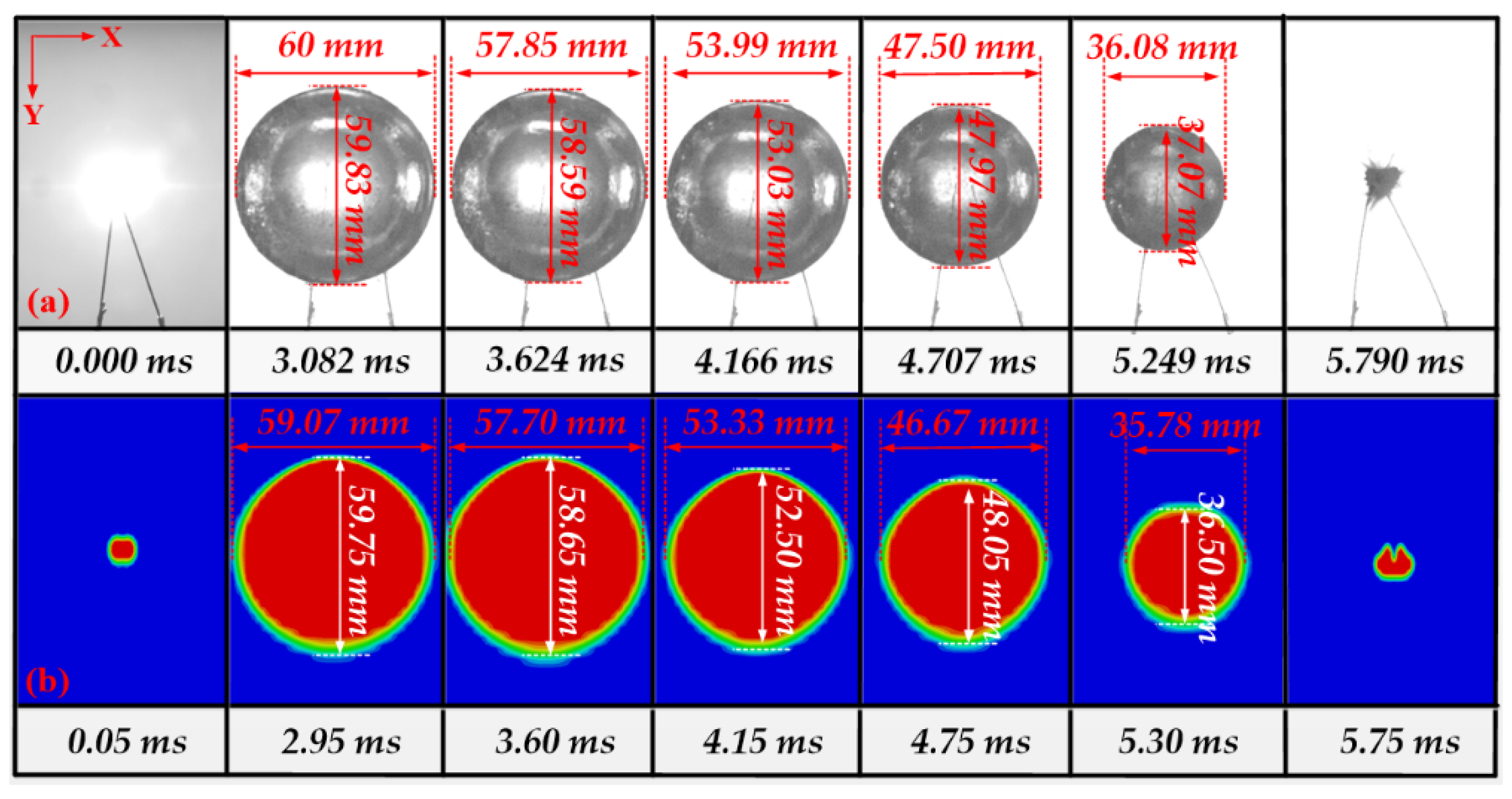
In this study, free-field cavitation bubbles, cavitation bubbles near the flat plate target, and cavitation bubbles near the hemispherical target were simulated. The specific experimental statuses are shown in

Table 2. Experimental statuses.

	Free Field	Flat Plate Target	Hemispherical Target
Discharge voltage	400 V	400 V	400 V
Explosion source water depth	265 mm	265 mm	265 mm
Explosion distance	—	10 mm	10 mm
		25 mm	25 mm

. The following will discuss the simulation effects of simulation in these three states.

4.1. Free Field

The pulsation process of free-field cavitation bubbles is simpler than that of cavitation bubbles near the boundary. Thus, we firstly used simulation to simulate the pulsation process of free-field cavitation bubbles. This research simulated the free-field bubble pulsation process with simulation and did not simulate the process from the explosion source to the shock wave propagation. However, the simulation reflected the combined effects of gravity and buoyancy on bubble pulsation, especially during bubble collapse and jet formation. Figure 8 shows how similar the simulated bubble and the experimental bubble were in terms of bubble morphology, according to the bubble image taken by the high-speed camera. At t(a) = 0 ms, a dazzlingly bright light was emitted at the intersection of the electrodes, and electric spark bubbles began to form. At t(a) = 3.082 ms, the bubble reached its maximum volume, and the bubble radius at that time was 60 mm. After that, the bubble began to enter the contraction phase of the first cycle. When 3.624 ms < t(a) < 5.249 ms, the bubbles shrank to a spherical shape. The collapse phase of the first cycle of the bubble occurred at t(a) = 5.79 ms. This can be seen in the simulation results. When t(b) = 0.05 ms, a high-temperature and high-pressure bubble was formed, and then its internal pressure dropped rapidly. When t(b) = 2.95 ms, the simulated bubble reached the maximum volume, and the bubble radius at that time was 59.07 mm. After that, the simulated bubble entered the contraction phase of the first cycle. The collapse phase of the first cycle of the simulated bubble occurred at t(b) = 5.75 ms. These characteristics are similar to the results obtained by Cole in 1948. At the same time, these characteristics are similar to the experimental results. The range of the tolerance T between the image time obtained from the numerical simulation and the image time obtained from the experiment was 0.016 ms ≤ T ≤ 0.132 ms. T was much smaller than the experimental time and simulation time (5.75 ms). Thus, it can be deduced that the author used the numerical results at similar moments in the experiment for comparison.

Assuming the same bubble shape, the average error ($\left|\overline{T}\right|$) between the experimental measurement time and the simulation time is calculated using Equation (16):

$$\left|\overline{T}\right|=\left|\frac{\left(t_{a1}-t_{b1}\right)+\left(t_{a2}-t_{b2}\right)+\dots +\left(t_{an}-t_{bn}\right)}{n}\right|$$

(22)

According to Equation (16), when the bubble shapes are similar, the average error $\left|\overline{T}\right|$ between the experimental measurement time and the simulation time is 0.05 ms. The experiment measured that the pulsation time of the first cycle of the bubble was 5.79 ms. $\left|\overline{T}\right|$ accounts for only 0.8% of 5.79 ms and is acceptable. Let $\left|\overline{L_x}\right|$ be the size error of the same bubble shape in terms of x level, and let $\left|\overline{L_y}\right|$ be the size error of the same bubble shape in terms of y level. When the bubble shape is the same, we use Equations (23) and (24) to calculate the average error $\left|\overline{L_x}\right|$ and $\left|\overline{L_y}\right|$ between the experimentally measured bubble size and the simulated bubble size:

$$\left|\overline{L_x}\right|=\left|\frac{\left(L_{ax1}-L_{bx1}\right)+\left(L_{ax2}-L_{bx2}\right)+\dots +\left(L_{axn}-L_{bxn}\right)}{n}\right|$$

(23)

$$\left|\overline{L_y}\right|=\left|\frac{\left(L_{ay1}-L_{by1}\right)+\left(L_{ay2}-L_{by2}\right)+\dots +\left(L_{ayn}-L_{byn}\right)}{n}\right|$$

(24)

According to Equations (23) and (24), when the bubble shapes were similar, the average errors $\left|\overline{L_x}\right|$ and $\left|\overline{L_y}\right|$ between the experimentally measured bubble size and the simulated bubble size were 0.574 mm and 0.264 mm, respectively. The maximum values of bubbles in the X direction and Y direction measured by the experiment were 60 mm and 59.83 mm, respectively. In the research, the error was less than 10% in order to meet the requirements. $\left|\overline{L_x}\right|$ and $\left|\overline{L_y}\right|$ only accounted for 0.9% and 0.4% (less than 10%) of 60 mm and 59.83 mm and the results were acceptable.

In simulation, the grid is fixed and does not move; only the materials flowing between the grids move. ABAQUS describes the movement of materials in the Euler body by calculating the Eulerian Volume Fraction (EVF) in every grid. If the EVF of a material in the grid is 1, it means the grid is filled with this material. If the EVF of a material in the grid is less than 1, it means that there are other materials in the grid, or it is empty. We can see the percentage of material in each grid through the legend.

Figure 9 shows the curve of the bubble radius of the horizontal direction in the first pulse cycle of the bubble over time. The red triangles are the experimental results. The experimental bubble size was measured by a ruler, as shown in Figure 10. The space rectangular coordinate system was established with the center of the bottom of the water tank as the origin. In the above JWL equation, we set the center of the initial high-pressure bubble to (0, 0, 0.265). The blue line is the simulation result. As for the curve, the experimental result is the same as the development trend of the simulation results. The numerical results were very similar.

In 2010, Prior and Brown [41] derived an empirical equation describing the amplitude and period of the cavitation bubble pulsation, as shown below:

$$R=3.4{\left(\frac{W}{Z+10.1}\right)}^{1/3}$$

(25)

where R is the maximal bubble radius.

$$T=K\frac{W^{1/3}}{{\left(Z+10.1\right)}^{5/6}}\left(1-\frac{R}{5Z}\right)$$

(26)

where T is the time of the bubble’s first pulse. For the high-pressure bubbles generated by TNT, we chose the parameter K = 2.11. Using Equations (25) and (26), we calculated that the maximum radius of the bubble was 33.60 mm, and the pulsation time of the first cycle of the bubble was 4.834 ms. These results are similar to those predicted using simulation. However, there are some differences. In this research, we assumed that the initial radius of the bubble was the same as the radius of the high-pressure bubble, and the initial bubble expansion velocity was 0 m/s. We think that these simplified settings might have affected the accuracy of the simulation. Therefore, if the initial condition of the bubble is set as a practical situation, the results simulated by the finite element method will be closer to reality. The numerical model solves this problem by setting the gravity parameters of the entire area. GEOSTATIC* can be entered into ABAQUS 6.14 to obtain the static balance of the experimental water area quickly. Figure 11 shows how the distance between the upper and lower edges of the bubble in simulation changed over time. Although there are slight differences between the numerical simulation results and the experimental results, the curves they constitute are similar. During the first pulsation period of the bubble, the upward migration of the numerical simulation bubble and the experimental bubble was very small.

ABAQUS 6.14 can simulate the bubble shape in the collapse stage in detail. During the bubble collapse stage, different parts of the bubble shrink at different rates. This unequal shrinkage speed causes the top surface of the bubble to deform and produce a downward jet. Due to the pressure, the water at the top of the bubble rushes into the jet that is being formed, having an impact on the bottom bubble wall. When the bubble begins to shrink and until the jet breaks through the bottom bubble wall, the bubble gradually changes from a spherical shape to a ring shape. Figure 12 shows the image formed by the jet during the bubble collapse stage. At this stage, the bubble area undergoes drastic flow changes. Figure 13 shows the velocity field formed by the jet during the bubble collapse stage. The velocity field shows the size and direction of the jet. Here, we call the bubble form a jet, but the jet does not break through the bottom bubble as a single connected bubble. We call the annular bubble a double connected bubble. At t = 6.1 ms, the single connected bubble became a double connected bubble.

4.2. Flat Plate Target

In this section, we discuss the reliability of the simulation of cavitation bubbles from two explosion distances. The two explosion distances are 10 mm and 25 mm, respectively. That is, γ = 0.33 and γ = 0.83.

4.2.1. γ = 0.33 in Flat Plate Target

The pulsation process of cavitation bubbles near the flat plate target is more complicated than that of the free field, but simpler than that of the hemisphere target. Thus, next we used ABAQUS/Explicit to simulate the pulsation process of cavitation bubbles near the flat plate target. The process was the same as for the free field. The simulation reflected the combined effects of gravity, buoyancy, and the Bjerknes force on bubble pulsation, especially during bubble collapse and jet formation. Figure 14 shows how similar the simulated bubble and the experimental bubble were in terms of bubble morphology, according to the bubble image taken by the high-speed camera. At t(a) = 0.003 ms, a dazzlingly bright light was emitted at the intersection of the electrodes, and electric spark bubbles began to form. At t(a) = 4.208 ms, the bubble reached its maximum volume, and the bubble radius at that time was 60 mm. After that, the bubble began to enter the contraction phase of the first cycle. When 4.874 ms < t(a) < 6.916 ms, the bubbles shrank into an inverted mound shape. The collapse phase of the first cycle of the bubble occurred at t(a) = 7.582 ms. This can be seen in the simulation results. When t(b) = 0.005 ms, a high-temperature and high-pressure bubble was formed, and then the internal pressure dropped rapidly. When t(b) = 4.15 ms, the simulated bubble reached the maximum volume; the bubble radius at that time was 59.52 mm. After that, the ABAQUS/Explicit simulated bubble entered the contraction phase of the first cycle. The collapse phase of the first cycle of the ABAQUS-Euler simulated bubble occurred at t(b) = 6.9 ms. These characteristics were similar to the experimental results. The range of the tolerance T between the image time obtained from the numerical simulation and the image time obtained from the experiment was 0.002 ms ≤ t ≤ 0.282 ms. T was much smaller than the experimental time (7.582 ms) and the simulation time (7.3 ms).

According to Equation (16), when the bubble shapes were similar, the average error $\left|\overline{T}\right|$ between the experimental measurement time and the simulation time was 0.095 ms. The pulsation time of the first cycle of the bubble was 7.582 ms. $\left|\overline{T}\right|$ accounts for only 1.2% of 7.582 ms and is acceptable. According to Equations (23) and (24), when the bubble shapes were similar, the average errors $\left|\overline{L_x}\right|$ and $\left|\overline{L_y}\right|$ between the experimentally measured bubble size and the ABAQUS/Explicit simulated bubble size were 0.294 mm and 0.406 mm, respectively. The maximum values of bubbles in the X direction and Y direction measured by the experiment were 60 mm and 33.62 mm, respectively. $\left|\overline{L_x}\right|$ and $\left|\overline{L_y}\right|$ only account for 0.4% and 1.2% (less than 10%) of 60 mm and 33.62 mm and the results are acceptable.

Figure 15 shows how the distance between the upper and lower edges of the bubble in simulation changed over time. Although there are slight differences between the numerical simulation results and the experimental results, the curves they constitute are similar. During the first pulsation period of the bubble, the upward migration of the numerical simulation bubble and the experimental bubble were very small.

The Explicit domain in ABAQUS 6.14 used in this study could simulate the bubble shape in the collapse stage in detail. During the bubble collapse stage, different parts of the bubble shrink at different rates. Since the hydrostatic pressure of the lower part of the bubble is higher than that of the upper part, its lower part shrinks faster than the upper part. This unequal shrinkage speed causes the bottom surface of the bubble to deform and produce an upward jet. Due to the water pressure, the water at the bottom of the bubble rushes into the jet that is being formed, causing an impact on the top bubble wall. When the bubble begins to shrink and until the jet breaks through the top bubble wall, the bubble gradually changes from a hemispherical shape to a ring shape. Figure 16 shows the image formed by the jet during the bubble collapse stage. At this stage, the bubble area undergoes drastic flow changes. Figure 17 shows the velocity field formed by the jet during the bubble collapse stage. The velocity field shows the size and direction of the jet. Here, we call the bubble form a jet, but the jet does not break through the top bubble as a single connected bubble. We call the annular bubble a double connected bubble. At t = 7.3 ms, the single connected bubble became a double connected bubble.

4.2.2. γ = 0.83 in the Flat Plate Target

Figure 18 shows how similar the simulated bubble and the experimental bubble were in terms of bubble morphology, according to the bubble image taken by the high-speed camera. At t(a) = 0.499 ms, a dazzlingly bright light was emitted at the intersection of the electrodes, and electric spark bubbles began to form. At t(a) = 4.041 ms, the bubble reached its maximum volume; the bubble radius at that time was 60 mm. After that, the bubble began to enter the contraction phase of the first cycle. When 4.666 ms < t(a) < 6.124 ms, the bubbles shrank into an inverted cone shape. When t(a) = 6.665 ms, the electric spark bubbles formed an obvious upward jet. The collapse phase of the first cycle of the bubble occurred at t(a) = 7.04 ms.

The simulation results of ABAQUS/Explicit showed that when t(b) = 0.55 ms, a high-temperature and high-pressure bubble formed, and its internal pressure dropped rapidly. When t(b) = 3.6 ms, the simulated bubble reached its maximum volume; the bubble radius at that time was 59.51 mm. After that, the ABAQUS/Explicit simulated bubble entered the contraction phase of the first cycle. When t(b) = 6.5 ms, a clear jet could be seen. The collapse phase of the first cycle of the simulated bubble occurred at t(b) = 6.9 ms. One can see the obvious annular bubble formed after the jet broke through the top of the bubble. These characteristics were similar to the experimental results. The range of the tolerance T between the image time obtained from the numerical simulation and the image time obtained from the experiment was 0.051 ms ≤ T ≤ 0.441 ms. T was much smaller than the experimental time (7.040 ms) and simulation time (6.9 ms).

According to Equation (16), when the bubble shapes were similar, the average error $\left|\overline{T}\right|$ between the experimental measurement time and the simulation time was 0.233 ms. The pulsation time of the first cycle of the bubble was 7.040 ms. $\left|\overline{T}\right|$ accounted for only 3.3% of 7.040 ms and was acceptable. According to Equations (17) and (18), when the bubble shapes were similar, the average errors $\left|\overline{L_x}\right|$ and $\left|\overline{L_y}\right|$ between the experimentally measured bubble size and the ABAQUS/Explicit simulated bubble size were 0.696 mm and 0.344 mm, respectively. The maximum values of bubbles in the X direction and Y direction measured by the experiment were 60 mm and 53.66 mm, respectively. $\left|\overline{L_x}\right|$ and $\left|\overline{L_y}\right|$ only accounted for 1.1% and 0.6% (less than 10%) of 60 mm and 53.66 mm and the results were acceptable.

Figure 19 shows how the distance between the upper and lower edges of the bubble in simulation changed over time. Although there are slight differences between the numerical simulation results and the experimental results, the curves they constitute are similar. During the first pulsation period of the bubble, the upward migration of the numerical simulation bubble and the experimental bubble were very small.

The Explicit domain in ABAQUS 6.14 used in this study could simulate the bubble shape in the collapse stage in detail. During the bubble collapse stage, different parts of the bubble shrink at different rates. Since the hydrostatic pressure of the lower part of the bubble is higher than that of the upper part, its lower part shrinks faster than the upper part. This unequal shrinkage speed causes the bottom surface of the bubble to deform and produce an upward jet. Due to the water pressure, the water at the bottom of the bubble rushes into the jet that is being formed, causing an impact on the top bubble wall. When the bubble begins to shrink and until the jet breaks through the top bubble wall, the bubble gradually changes from a spherical shape to a ring shape. Figure 20 shows the image formed by the jet during the bubble collapse stage. At this stage, the bubble area undergoes drastic flow changes. Figure 21 shows the velocity field formed by the jet during the bubble collapse stage. The velocity field shows the size and direction of the jet. Here, we call the bubble form a jet, but the jet does not break through the top bubble as a single connected bubble. We call the annular bubble a double connected bubble. At t = 6.55 ms, the single connected bubble became a double connected bubble.

4.3. Hemisphere Target

In this section, we discuss the reliability of simulation of cavitation bubbles from two explosion distances. The two explosion distances are 10 mm and 25 mm, respectively. That is, γ = 0.33 and γ = 0.83.

4.3.1. γ = 0.33 in the Hemisphere Target

The pulsation process of underwater explosion bubbles near the curved surface boundary is very complicated, and many influencing factors need to be considered. This research simulated the bubble pulsation process near the hemispherical boundary with simulation and did not simulate the process from the explosion source to the shock wave propagation. However, the simulation reflected the combined effects of gravity, buoyancy, and the Bjerknes force on bubble pulsation, especially during bubble collapse and jet formation. Figure 22 shows how similar the simulated bubble and the experimental bubble were in terms of bubble morphology, according to the bubble image taken by the high-speed camera. At t(a) = 0.041 ms, a dazzlingly bright light was emitted at the intersection of the electrodes, and electric spark bubbles began to form. At t(a) = 3.291 ms, the bubble reached its maximum volume; the bubble radius at that time was 60 mm. After that, the bubble began to enter the contraction phase of the first cycle. When t(a) = 29.64 ms, the bubbles shrank into an inverted mushroom shape. The collapse phase of the first cycle of the bubble occurred at t(a) = 6.290 ms. This can be seen in the simulation results of ABAQUS/Explicit. When t(b) = 0.050 ms, a high-temperature and high-pressure bubble was formed, and its internal pressure dropped rapidly. When t(b) = 3.400 ms, the simulated bubble reached its maximum volume; the bubble radius at that time was 57.16 mm. After that, the ABAQUS/Explicit simulated bubble entered the contraction phase of the first cycle. The collapse phase of the first cycle of the simulation bubble occurred at t(b) = 6.300 ms. These characteristics were similar to the experimental results. The range of the tolerance T between the image time obtained from the numerical simulation and the image time obtained from the experiment was 0.009 ms ≤ t ≤ 0.857 ms. T was much smaller than the experimental time and simulation time (6.3 ms).

According to Equation (16), when the bubble shapes were similar, the average error $\left|\overline{T}\right|$ between the experimental measurement time and the simulation time was 0.302 ms. The pulsation time of the first cycle of the bubble was 6.290 ms. $\left|\overline{T}\right|$ accounts for only 4.8% of 6.290 ms and was acceptable.

According to Equations (23) and (24), when the bubble shapes were similar, the average errors $\left|\overline{L_x}\right|$ and $\left|\overline{L_y}\right|$ between the experimentally measured bubble size and the ABAQUS/Explicit simulated bubble size were 0.368 mm and 1.626 mm, respectively. The maximum values of bubbles in the X direction and Y direction measured by the experiment were 60 mm and 35.56 mm, respectively. $\left|\overline{L_x}\right|$ and $\left|\overline{L_y}\right|$ only account for 0.6% and 4.5% (less than 10%) of 60 mm and 35.56 mm and the results were acceptable.

Figure 23 shows the curve of the bubble diameter in the horizontal direction in the first pulse cycle of the bubble over time. The blue line is the experimental measurement result. Since the bubble was not completely spherically symmetric during the explosion, we could only approximate the radius of the bubble. The space rectangular coordinate system was established with the center of the bottom of the water tank as the origin. In the above JWL equation, we set the initial position of the high-temperature and high-pressure initial bubble to (0, 0, 0.265). Ignoring the floating of the bubble during the explosion, this point was taken as the center of the bubble. The upper surface of the bubble has a boundary, and the distance between the center of the bubble and the boundary was less than the maximum radius of the cavitation bubble. After the upper surface of the bubble contacts the boundary, it will not continue to expand. Therefore, we can only measure the radius change of the bubble from the bottom surface of the bubble. Querying the value of the bottom surface center of each frame of the bubble, the coordinate value of this point can be obtained as (0, 0, x). X is the distance between the bottom surface of the bubble and the bottom of the water tank in each frame. We can calculate the radius of the bubble via r = 0.265 − x. The red line is the simulation result. From the curved point of view, the experimental result is the same as the development trend of the simulation result. The numerical results are very similar.

Using Equations (25) and (26), we calculated that the maximum radius of the bubble was 33.60 mm, and the pulsation time of the first cycle of the bubble was 4.834 ms. These results are similar to those predicted using ABAQUS/Explicit. In this research, we assumed that the initial radius of the bubble was the same as the radius of the explosion source, and the initial bubble expansion velocity was 0 m/s. We think that these simplified settings might have affected the accuracy of ABAQUS/Explicit. Therefore, if the initial condition of the bubble is set as a practical situation, the results simulated by the finite element method will be closer to reality. The numerical model solves this problem by setting the gravity parameters of the entire area. GEOSTATIC* can be entered into ABAQUS 6.14 to obtain the static balance of the water area quickly. Figure 24 shows how the distance between the upper and lower edges of the bubble in simulation changed over time. Although there are slight differences between the numerical simulation results and the experimental results, the curves they constitute are similar. During the first pulsation period of the bubble, the upward migration of the numerical simulated bubble and the experimental bubble was very small.

The Euler domain in ABAQUS 6.14 used in this study could simulate the bubble shape in the collapse stage in detail. During the bubble collapse stage, different parts of the bubble shrink at different rates. Since the hydrostatic pressure of the lower part of the bubble is higher than that of the upper part, its lower part shrinks faster than the upper part. This unequal shrinkage speed causes the bottom surface of the bubble to deform and produce an upward jet. Due to water pressure, the water at the bottom of the bubble rushes into the jet that is being formed, causing an impact on the top bubble wall. When the bubble begins to shrink and until the jet breaks through the top bubble wall, the bubble gradually changes from a spherical shape to a ring shape. Figure 25 shows the image formed by the jet during the bubble collapse stage. At this stage, the bubble area undergoes drastic flow changes. Figure 26 shows the velocity field formed by the jet during the bubble collapse stage. The velocity field shows the size and direction of the jet. Here, we call the bubble form a jet, but the jet does not break through the top bubble as a single connected bubble. We call the annular bubble a double connected bubble. At t = 6.1 ms, the single connected bubble became a double connected bubble.

4.3.2. γ = 0.83 in the Hemisphere Target

Figure 27 shows how similar the simulated bubble and the experimental bubble were in terms of bubble morphology, according to the bubble image taken by the high-speed camera. At t(a) = 0.000 ms, a dazzlingly bright light was emitted at the intersection of the electrodes, and electric spark bubbles began to form. At t(a) = 3.041 ms, the bubble reached its maximum volume; the bubble radius at that time was 60 mm. After that, the bubble began to enter the contraction phase of the first cycle. When 3.624 ms < t(a) < 5.499 ms, the bubbles shrank into an inverted oval shape. The collapse phase of the first cycle of the bubble occurred at t(a) = 6.082 ms.

From the simulation results of ABAQUS/Explicit, we can see that when t(b) = 0.05 ms, a high-temperature and high-pressure bubble was formed, and its internal pressure dropped rapidly. When t(b) = 2.95 ms, the simulated bubble reached its maximum volume; the bubble radius at that time was 59.04 mm. After that, the ABAQUS/Explicit simulated bubble entered the contraction phase of the first cycle. The collapse phase of the first cycle of the simulated bubble occurred at t(b) = 6.05 ms. A clear jet could also be seen at that time. These characteristics are similar to the experimental results. The range of the tolerance T between the image time obtained from the numerical simulation and the image time obtained from the experiment was 0.024 ms ≤ T ≤ 0.099 ms. T was much smaller than the experimental time (6.082 ms) and simulation time (6.05 ms).

According to Equation (16), when the bubble shapes were similar, the average error $\left|\overline{T}\right|$ between the experimental measurement time and the simulation time was 0.06 ms. The pulsation time of the first cycle of the bubble was 6.082 ms. $\left|\overline{T}\right|$ accounts for only 0.9% of 6.082 ms and is acceptable. According to Equations (23) and (24), when the bubble shapes were similar, the average errors $\left|\overline{L_x}\right|$ and $\left|\overline{L_y}\right|$ between the experimentally measured bubble size and the ABAQUS/Explicit simulated bubble size were 1.224 mm and 1.334 mm, respectively. The maximum values of bubbles in the X and Y directions measured by the experiment were 60 mm and 54.03 mm, respectively. $\left|\overline{L_x}\right|$ and $\left|\overline{L_y}\right|$ only account for 2% and 2.4% (less than 10%) of 60 mm and 54.03 mm, and the results are acceptable.

Figure 28 shows how the distance between the upper and lower edges of the bubble in simulation changed over time. Although there are slight differences between the numerical simulation results and the experimental results, the curves they constitute are similar. During the first pulsation period of the bubble, the upward migration of the numerical simulated bubble and the experimental bubble were very small.

The Explicit domain in ABAQUS 6.14 used in this study could simulate the bubble shape in the collapse stage in detail. During the bubble collapse stage, different parts of the bubble shrink at different rates. Since the boundary has a certain attraction to the top of the bubble, the upper part of the bubble forms an upward jet. In addition, since there is a certain distance between the boundary and the bubble, the attraction of the boundary to the bottom of the bubble becomes worse, so the lower part of the bubble forms a downward jet. When the bubble begins to shrink until the jet breaks through the bubble walls at the top and bottom, the bubble gradually changes from an oval shape to a double ring shape. Figure 29 shows the image formed by the jet during the bubble collapse stage. At this stage, the bubble area undergoes drastic flow changes. Figure 30 shows the velocity field formed by the jet during the bubble collapse stage. The velocity field shows the size and direction of the jet. Here, we call the bubble form a jet, but the jet does not break through the top bubble as a single connected bubble. We call the annular bubble a double connected bubble. At t = 6.05 ms, the single connected bubble became a double connected bubble.

Numerical calculations are widely used to predict possible cavitation bubble dynamics. The disadvantage of the simulation in solving the cavitation bubble dynamic problem is that it requires a lot of calculation resources. The advantage of the simulation is that it can solve nonlinear problems. When studying cavitation bubble dynamics, the bubble dynamics of the first pulsation period of the bubble are extremely important because they are related to the formation of jets. The jet will usually cause severe damage to nearby structures; therefore, it is necessary to study the flow of liquid around the bubble during the bubble collapse stage. ABAQUS/Explicit can be used to analyze it effectively. Advances in computer technology have reduced the time required to perform such simulations, making simulation calculations possible. The simulation model in this research was performed on a workstation with an Intel(R) Core (TM) i7-8700 K CPU, a 3.70 GHz processor, 16 GB RAM, 64-bit Microsoft Windows 10, and a 1.5 TB hard disk. The ABAQUS version used was 6.14-4, and the total computing time was 13 h 50 min.

The model accuracy of the simulation method meets the requirements of studying cavitation bubble dynamics. However, the research on cavitation bubble dynamics is only qualitative thus far.

5. Conclusions

This research used the Euler analysis technique in the ABAQUS/Explicit 6.14 program to reproduce the main bubble motion states in the experiment. Comparing the numerical simulation results with the experimental results, we found that the numerical model can effectively reproduce the basic characteristics of the bubble in the first pulsation stage. The first oscillation period of the bubble and the maximum radius of the bubble are generally similar to the experimental data. In addition, this paper also studies the velocity field of the liquid around the bubble, and the jet formation process during the bubble collapse stage.

Although factors such as incompressible non-viscous liquids and the initial idealization of underwater explosion bubbles were set in the numerical research, the simplified model simulated most of the important pulsation processes of underwater explosion bubbles. It includes the pulsation of the first cycle of the bubble and the jet generated during the bubble collapse stage for the pulsation process of spark bubbles in the free field and two kinds of wall boundary conditions. The numerical model reproduced the characteristics of bubble motion, including jets, bubble rings, etc. However, the simulation difficulty differed between the three boundary conditions. The simulation of cavitation bubbles near the hemispherical target was the most difficult, followed by the flat target. The free field was the simplest. This was determined by the complexity of the force of the cavitation bubble. The numerical model also analyzed the evolution of the velocity field in the process of nonlinear interaction in detail. In the bubble collapse stage, the high-speed jet was simulated, and the velocity field at this time was analyzed. The influence of the dimensionless burst distance parameter on the pulsation of the bubble under different conditions was studied.

This research discusses the application of simulation (e.g., ABAQUS 6.14), that is, quantitative modeling was performed in the vicinity of the free field, the flat plate boundary, and the curved surface boundary to simulate the electric spark bubble dynamic. This numerical simulation method is also suitable for different types of explosives, explosive charges, and explosive locations.

References

1. Wang, S.-P.; Zhang, A.-M.; Liu, Y.-L.; Zhang, S.; Cui, P. Bubble dynamics and its applications. J. Hydrodyn. 2018, 30, 975–991. [Google Scholar] [CrossRef]
2. Gibson, D.C.; Blake, J.R. Growth and collapse of cavitation bubble near flexible boundaries. In Proceedings of the 7th Australasian Hydraulics and Fluid Mechanics Conference, Brisbane, Australia, 18–22 August 1980. [Google Scholar]
3. Han, R.; Tao, L.; Zhang, A.M.; Li, S. Experimental and numerical investigation of the dynamics of a coalesced oscillating bubble near a free surface. Ocean Eng. 2019, 186, 106096. [Google Scholar] [CrossRef]
4. Goh, B.H.T.; Gong, S.W.; Ohl, S.-W.; Khoo, B.C. Spark-generated bubble near an elastic sphere. Int. J. Multiph. Flow 2017, 90, 156–166. [Google Scholar] [CrossRef]
5. Ma, X.; Huang, B.; Zhao, X.; Wang, Y.; Chang, Q.; Qiu, S.; Fu, X.; Wang, G. Comparisons of spark-charge bubble dynamics near the elastic and rigid boundaries. Ultrason. Sonochem. 2018, 43, 80–90. [Google Scholar] [CrossRef]
6. Zhang, M.; Chang, Q.; Ma, X.; Wang, G.; Huang, B. Physical investigation of the counterjet dynamics during the bubble rebound. Ultrason. Sonochem. 2019, 58, 104706. [Google Scholar] [CrossRef]
7. Ma, C.L.; Shi, D.Y.; Li, C.; Wang, M.N.; He, D.Z. Experimental Research on the Electric Spark Bubble Load Characteristics under the Oblique 45 Degree Curved Surface Boundary. J. Mar. Sci. Eng. 2021, 9, 32. [Google Scholar] [CrossRef]
8. Cui, P.; Wang, Q.X.; Wang, S.P.; Zhang, A.M. Experimental study on interaction and coalescence of synchronized multiple bubbles. Phys. Fluids 2016, 28, 012103. [Google Scholar] [CrossRef] [Green Version]
9. Tian, Z.-L.; Liu, Y.-L.; Zhang, A.M.; Tao, L.; Chen, L. Jet development and impact load of underwater explosion bubble on solid wall. Appl. Ocean Res. 2020, 95, 102013. [Google Scholar] [CrossRef]
10. Zhang, A.M.; Wang, S.-P.; Huang, C.; Wang, B. Influences of initial and boundary conditions on underwater explosion bubble dynamics. Eur. J. Mech. B/Fluids 2013, 42, 69–91. [Google Scholar] [CrossRef]
11. Ma, C.L.; Shi, D.Y.; Chen, Y.Y.; Cui, X.W.; Wang, M.N. Experimental Research on the Influence of Different Curved Rigid Boundaries on Electric Spark Bubbles. Materials 2020, 13, 3941. [Google Scholar] [CrossRef]
12. Phan, T.H.; Nguyen, V.T.; Park, W.G. Numerical study on strong nonlinear interactions between spark-generated underwater explosion bubbles and a free surface. Int. J. Heat Mass Transf. 2020, 163, 120506. [Google Scholar] [CrossRef]
13. Costanzo, F.; Surface, N.; Boulevard, M. Underwater Explosion Phenomena and Shock Physics. In Structural Dynamics; Springer: New York, NY, USA, 2011; Volume 3, pp. 917–938. [Google Scholar]
14. Tian, Z.-L.; Liu, Y.-L.; Zhang, A.M.; Tao, L. Energy dissipation of pulsating bubbles in compressible fluids using the Eulerian finite-element method. Ocean Eng. 2020, 196, 106714. [Google Scholar] [CrossRef]
15. Daramizadeh, A.; Ansari, M.R. Numerical simulation of underwater explosion near air–water free surface using a five-equation reduced model. Ocean Eng. 2015, 110, 25–35. [Google Scholar] [CrossRef]
16. Beig, S.A.; Aboulhasanzadeh, B.; Johnsen, E. Temperatures produced by inertially collapsing bubbles near rigid surfaces. J. Fluid Mech. 2018, 852, 105–125. [Google Scholar] [CrossRef]
17. Wu, W.B.; Zhang, A.M.; Liu, Y.L.; Wang, S.P. Local discontinuous Galerkin method for far-field underwater explosion shock wave and cavitation. Appl. Ocean Res. 2019, 87, 102–110. [Google Scholar] [CrossRef]
18. Qin, Z.; Alehossein, H. Heat transfer during cavitation bubble collapse. Appl. Therm. Eng. 2016, 105, 1067–1075. [Google Scholar] [CrossRef]
19. Petrov, N.V.; Schmidt, A.A. Multiphase phenomena in underwater explosion. Exp. Therm. Fluid Sci. 2015, 60, 367–373. [Google Scholar] [CrossRef]
20. Simulia ABAQUS 6.11. ABAQUS Analysis User’s Manual; HKS Inc.: Providence, RI, USA, 2011. [Google Scholar]
21. Ma, C.; Shi, D.; Cui, X.; Chen, Y. A New Measurement Based on HPB to Measure the Wall Pressure of Electric-Spark-Generated Bubble near the Hemispheric Boundary. Shock. Vib. 2020, 2020, 1–20. [Google Scholar] [CrossRef] [Green Version]
22. Lew, K.S.F.; Klaseboer, E.; Khoo, B.C. A collapsing bubble-induced mircopump: An experimental study. Sens. Actuators A 2007, 133, 161–172. [Google Scholar] [CrossRef]
23. Brujan, E.A.; Keen, G.S.; Vogel, A.; Blake, J.R. The final stage of the collapse of a cavitation bubble close to a rigid boundary. Phys. Fluids 2002, 14, 1. [Google Scholar] [CrossRef] [Green Version]
24. Pearson, A.; Cox, E.; Blake, J.R.; Otto, S.R. Bubble interactions near a free surface. Eng. Anal. Bound Elem. 2004, 28, 295–313. [Google Scholar] [CrossRef]
25. Liu, N.N.; Ming, F.R.; Liu, L.T.; Ren, S.F. The dynamic behaviors of a bubble in a confined domain. Ocean Eng. 2017, 144, 175–190. [Google Scholar] [CrossRef]
26. Li, Z.-R.; Sun, L.; Zong, Z.; Dong, J. A boundary element method for the simulation of non-spherical bubbles and their interactions near a free surface. Acta Mech. Sin. 2012, 28, 51–65. [Google Scholar] [CrossRef]
27. Liu, N.N.; Cui, P.; Ren, S.F.; Zhang, A.M. Study on the interactions between two identical oscillation bubbles and a free surface in a tank. Phys. Fluids 2017, 29, 052104. [Google Scholar] [CrossRef]
28. Wang, S.; Duan, W.; Wang, Q. The bursting of a toroidal bubble at a free surface. Ocean Eng. 2015, 109, 611–622. [Google Scholar] [CrossRef]
29. Zhang, Y.L.; Yeo, K.S.; Khoo, B.C.; Wang, C. 3D jet impact and toroidal bubbles. J. Compt. Phys. 2001, 166, 336–360. [Google Scholar] [CrossRef]
30. Zhang, Y.L.; Yeo, K.S.; Khoo, B.C.; Chong, W.K. Three-dimensional computation of bubbles near a free surface. J. Compt. Phys. 1998, 146, 105–123. [Google Scholar] [CrossRef]
31. Wang, Q.X.; Yeo, K.S.; Khoo, B.C.; Lam, K.Y. Vortex ring modeling of toroidal bubbles. Theor. Comput. Fluid Dyn. 2005, 19, 303–317. [Google Scholar] [CrossRef]
32. Zhang, A.M.; Yao, X.L.; Li, J. The interaction of an underwater explosion bubble and an elastic–plastic structure. Appl. Ocean Res. 2008, 30, 159–171. [Google Scholar] [CrossRef]
33. Li, J.; Rong, J.-L. Bubble and free surface dynamics in shallow underwater explosion. Ocean Eng. 2011, 38, 1861–1868. [Google Scholar] [CrossRef]
34. Chisum, J.E.; Shin, Y.S. Explosion gas bubbles near simple boundaries. Shock Vib. 1997, 4, 11–25. [Google Scholar] [CrossRef]
35. Abe, A.; Katayama, M.; Murata, K.; Kato, Y.; Tanaka, K. Numerical study of underwater explosions and following bubble pulses. In Proceedings of the 15th APS Topical Conference on Shock Compression of Condensed Matter, Kohala Coast, HI, USA, 24–29 June 2007. [Google Scholar]
36. Barras, G.; Souli, M.; Aquelet, N.; Couty, N. Numerical simulation of underwater explosions using an ALE method. The pulsating bubble phenomena. Ocean Eng. 2012, 41, 53–66. [Google Scholar] [CrossRef]
37. Plesset, M.S.; Prosperetti, A. Bubble dynamics and cavitation. Ann. Rev. Fluid Mech. 1997, 9, 145–185. [Google Scholar] [CrossRef]
38. Simulia, D. Abaqus Version 2016 Documentation; Dassault Systems Simulia Corp: Providence, RI, USA, 2012. [Google Scholar]
39. Li, X.; Zhang, C.; Wang, X. Research on the Influence of Water State Equation on Underwater Explosion. Eng. Mech. 2014, 31, 46–52. [Google Scholar]
40. Prior, M.K.; Brown, D.J. Estimation of depth and yield of underwater explosions from first and second 826 bubble-oscillation periods. Ocean. Eng. 2010, 35, 103–112. [Google Scholar] [CrossRef]
41. Shen, F.; Wang, H.; Yuan, J. A Simple Algorithm for Determining the Parameters of JWL State Equation. Vib. Shock. 2014, 9, 107–110. [Google Scholar]
Figure 1. The pulsation process of cavitation bubbles affected by buoyancy.
Jmse 09 00619 g001
Figure 2. An experimental device for the occurrence and measurement of electric spark bubbles: (a) Schematic; (b) Real products.
Jmse 09 00619 g002
Figure 3. Comparison of spark bubble expansion to maximum volume and explosive bubble expansion to maximum volume: (a) The state before high voltage discharge; (b) The state of the explosive before the explosion; (c) The state where the electric spark bubble expands to its maximum volume; (d) The state where the explosive bubble expands to its maximum volume.
Jmse 09 00619 g003
Figure 4. The arrangement of the model: (a) Free field; (b) hemisphere target; (c) flat plate target.
Jmse 09 00619 g004
Figure 5. Finite element model of ABAQUS-Euler: (a) model main view; (b) model side view; (c) material distribution inside the Euler area of the hemisphere target; (d) enlarged view of the mesh around the hemisphere target; (e) material distribution inside the Euler area of the flat plate target; (f) enlarged view of the mesh around the flat plate target.
Jmse 09 00619 g005
Figure 6. The views of the peeler grid: (ac) The peeler grid of hemisphere target; (d,e) the peeler grid of the flat plate target.
Jmse 09 00619 g006
Figure 7. Cole calculation for TNT on the logarithmic plot.
Jmse 09 00619 g007
Figure 8. Pulsation chart of the first cycle of the bubble under free-field conditions: (a) Electric spark bubbles generated by 400 V high-voltage electric discharge; (b) high-pressure cavitation bubbles simulated by ABAQUS/Explicit.
Jmse 09 00619 g008
Figure 9. The relationship between the horizontal direction radius of the first pulse period of the free-field bubble and time. The red triangles are the experimental measurement results. The blue line is the ABAQUS/Explicit simulation result.
Jmse 09 00619 g009
Figure 10. Schematic diagram of the method of measuring bubble diameter [11].
Jmse 09 00619 g010
Figure 11. The position of the upper bubble surface and the lower bubble surface.
Jmse 09 00619 g011
Figure 12. Simulated bubble motion during the collapse phase at: (a) t = 5.55 ms; (b) t = 5.65 ms; (c) t = 5.70 ms; (d) t = 5.80 ms; (e) t = 5.90 ms; and (f) t = 6.10 ms.
Jmse 09 00619 g012
Figure 13. Velocity field in the bubble area during the collapse phase at: (a) t = 5.55 ms; (b) t = 5.60 ms; (c) t = 5.65 ms; and (d) t = 5.70 ms.
Jmse 09 00619 g013
Figure 14. A pulsation chart of the first cycle of the bubble when γ = 0.33 and ζ = 0: (a) Electric spark bubbles generated by 400 V high-voltage electric discharge; (b) high-pressure cavitation bubbles simulated by ABAQUS/Explicit.
Jmse 09 00619 g014
Figure 15. The position of the upper bubble surface and the lower bubble surface.
Jmse 09 00619 g015
Figure 16. Simulated bubble motion during the collapse phase at: (a) t = 7.3 ms; (b) t = 7.35 ms; (c) t = 7.4 ms; (d) t = 7.45 ms; (e) t = 7.55 ms; and (f) t = 7.9 ms.
Jmse 09 00619 g016
Figure 17. Velocity field in the bubble area during the collapse phase at: (a) t = 7.0 ms; (b) t = 7.4 ms; (c) t = 7.45 ms; and (d) t = 7.55 ms.
Jmse 09 00619 g017
Figure 18. A pulsation chart of the first cycle of the bubble when γ = 0.83 and ζ = 0: (a) Electric spark bubbles generated by 400 V high-voltage electric discharge; (b) high-pressure cavitation bubbles simulated by ABAQUS/Explicit.
Jmse 09 00619 g018
Figure 19. The position of the upper bubble surface and the lower bubble surface.
Jmse 09 00619 g019
Figure 20. Simulated bubble motion during the collapse phase at: (a) t = 6.55 ms; (b) t = 6.60 ms; (c) t = 6.70 ms; (d) t = 6.75 ms; (e) t = 6.80 ms; and (f) t = 6.90 ms.
Jmse 09 00619 g020
Figure 21. Velocity field in the bubble area during the collapse phase at: (a) t = 6.45 ms; (b) t = 6.55 ms; (c) t = 6.70 ms; and (d) t = 6.95 ms.
Jmse 09 00619 g021
Figure 22. A pulsation chart of the first cycle of the bubble when γ = 0.33 and ζ = 1.2: (a) Electric spark bubbles generated by 400 V high-voltage electric discharge; (b) high-pressure cavitation bubbles simulated by ABAQUS/Explicit.
Jmse 09 00619 g022
Figure 23. The relationship between the horizontal direction diameter of the bubble’s first pulse cycle and time when γ = 0.33 and ζ = 1.2. The blue line is the experimental measurement result. The red line is the ABAQUS/Explicit simulation result.
Jmse 09 00619 g023
Figure 24. The position of the upper bubble surface and the lower bubble surface.
Jmse 09 00619 g024
Figure 25. Simulated bubble motion during the collapse phase at: (a) t = 6.1 ms; (b) t = 6.2 ms; (c) t = 6.3 ms; (d) t = 6.4 ms; (e) t = 6.5 ms; and (f) t = 6.6 ms.
Jmse 09 00619 g025
Figure 26. Velocity field in the bubble area during the collapse phase at: (a) t = 6.0 ms; (b) t = 6.1 ms; (c) t = 6.2 ms; and (d) t = 6.3 ms.
Jmse 09 00619 g026
Figure 27. A pulsation chart of the first cycle of the bubble when γ=0.83 and ζ=1.2: (a) Electric spark bubbles generated by 400 V high-voltage electric discharge; (b) high-pressure cavitation bubbles simulated by ABAQUS/Explicit.
Jmse 09 00619 g027
Figure 28. The position of the upper bubble surface and the lower bubble surface.
Jmse 09 00619 g028
Figure 29. Simulated bubble motion during the collapse phase at: (a) t =6.05 ms; (b) t = 6.10 ms; (c) t = 6.15 ms; (d) t = 6.20 ms; (e) t = 6.35 ms; and (f) t = 6.60 ms.
Jmse 09 00619 g029
Figure 30. Velocity field in the bubble area during the collapse phase at: (a) t = 5.80 ms; (b) t = 5.85 m; (c) t = 5.90 ms; and (d) t = 6.00 ms.
Jmse 09 00619 g030