Abstract
A novel method for supervisory control of multilink manipulators mounted on underwater vehicles is considered. This method is designed to significantly increase the level of automation of manipulative operations, by the building of motion trajectories for a manipulator working tool along the surfaces of work objects on the basis of target indications given by the operator. This is achieved as follows: The operator targets the camera (with changeable spatial orientation of optical axis) mounted on the vehicle at the work object, and uses it to set one or more working point on the selected object. The geometric shape of the object in the work area is determined using clouds of points obtained from the technical vision system. Depending on the manipulative task set, the spatial motion trajectories and the orientation of the manipulator working tool are automatically set using the spatial coordinates of these points lying on the work object surfaces. The designed method was implemented in the C++ programming language. A graphical interface has also been created that provides rapid testing of the accuracy of overlaying the planned trajectories on the mathematically described surface of a work object. Supervisory control of an underwater manipulator was successfully simulated in the V-REP environment.
1. Introduction
Underwater unmanned vehicles (UUV) equipped with multilink manipulators (MM) are widely used in various research and technological operations in the world’s oceans. They facilitate the cleaning of underwater structures [1], diagnostics of underwater pipelines and cables [2,3], operations with subsea valve systems [3,4,5], collection of scientific material [6,7,8], archaeological surveys [9], cleaning of ship hulls from fouling [10], etc.
Modern trends in the design and operation of UUV are aimed at increasing their functional capabilities on the basis of novel technologies and methods for recognizing surrounding objects and for automatically building trajectories and modes of motion for both the UUV, and MM mounted on them [11,12,13,14]. Currently, the vast majority of underwater technological and research manipulative operations are performed only in a manual mode by specially trained UUV operators. Experienced operators successfully set trajectories for MM working tools [15,16,17]; nevertheless, it is very difficult for them to quickly and accurately solve a multitude of complex problems while having no direct contact with a work object and using only video images. This reduces the efficiency of their operation and increases the probability of errors.
This problem was also faced during deep-sea research expeditions in the Sea of Japan, Bering Sea, and Sea of Okhotsk, with the deployment of a Sub-Atlantic Comanche 18 remotely operated vehicle (ROV) equipped with a Schilling Orion 7P manipulator [18,19,20]. The routine collection of sediment (Figure 1), geological rock, and bacterial mat samples very often led to operator fatigue within a short period of time, to a significant increase in operation time, to errors in operations, and even to damage to working tools and samplers.
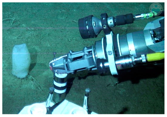
Figure 1.
A manipulative operation performed using a Schilling Orion 7P manipulator.
During manipulative operations, an UUV is exposed to undesirable dynamic impacts from the surrounding aquatic environment and the moving MM. These impacts shift the UUV position from the work object and complicate the control of the MM. To solve these problems, there are systems [21,22,23] that allow holding an UUV performing a manipulative operation in the desired spatial position with great accuracy. Moreover, if an MM has a greater number of degrees of mobility than is required for operations, the system [24] generates control signals for its actuators in such a way that this MM has the least impact on the UUV. These systems are indispensable for providing accurate operations in the UUV hovering mode. However, to facilitate manual control of MM, additional supervisory control systems are required.
To increase the efficiency of manipulative operations and reduce the load on operators, computer systems have been created [25] that allow operations to be performed on-line in a supervisory mode. In this control mode, the operator sets only simple target indications for the MM. Based on these indications, control signals for all the MM actuators are generated in a real-time mode. Some components of such systems have been tested on the ROV Jason [26]. To simplify the manual control of MMs, a strategy with the use of the P300 Brain–Computer Interface is proposed [27]. However, all the systems considered do not allow identification of the shape of the work objects or automatically building complex spatial motion trajectories of MM working tools over the surface of these objects.
With the development of technical vision systems (TVS) and environmental object recognition technologies, a new trend has arisen to increase the level of automation of many manipulative operations. The approach proposed in [28] is the use of a stereo camera mounted on the MM gripper, which allows determining the position and orientation of a known object with a pre-installed “Fiducial marker”. This work suggested automatic generation of MM control signals based on the obtained data that ensure firm gripping of objects with the correct orientation of the gripper. However, applying special markers to underwater objects is often impossible, which significantly limits the practical feasibility of this approach.
To facilitate spatial perception of work objects by the MM operator, the article [29] provides a method that allows composing a map of image depth with the use of two stereo cameras mounted on the UUV. This provides the operator with a three-dimensional (3D) view of the environment, which can be used to control the MM in an augmented reality mode. The approach considered in [30] is based on 3D scanning with two multibeam sonars, while the algorithm in [31] provides rapid reconstruction of the scanned surface, with filtering out noise in the data transferred from these echo-sounders. The above listed methods can be successfully applied to accurately determine the spatial positions and shapes of many underwater objects.
However, the existing systems and methods, while facilitating the operator’s perception of the surrounding underwater environment and simplifying the process of manual control of the MM, do not provide sufficiently automated building of the desired motion trajectories of the MM along the surface of underwater object and with the subsequent automatic performing of these trajectories with its working tools. Thus, the process of complex manipulative operations still requires MM operators to constantly control and perform necessary operative actions. This leads to operator fatigue within a short period of time, to a significant increase in the time needed for even standard operations, and often to serious errors and emergencies.
Due to the significant increase in the level of automation of numerous (especially standard) manipulative operations and work using UUV, the present study addresses the issue of developing a new method and algorithms to perform even complex underwater manipulative operations with a MM in a supervisory mode. The designed method should provide rapid building of motion trajectories for MM working tools on the basis of target indications given by the operator. These trajectories, built in an automatic mode, should be accurately passed by the MM working tool with the required orientation relative to the work objects. In this case, the operator, by targeting the optical axis of the video camera mounted on the rotary platform of the UUV, will set the start and end points of the trajectories of the working tool motion and the boundaries of the work object area on which these trajectories should then be projected, taking into account the shape and spatial position of this object. To facilitate the operator’s manipulations in the process of supervisory target indication, a graphical interface will be created, which, among other things, will allow rapid testing of the accuracy of overlaying the built trajectories on the mathematically described area of the work object’s surface.
2. Specifics of the Method for Supervisory Control of MM
Using this method (see Figure 2), the geometric shapes and positions of the objects in the work area are first determined using clouds of points obtained from the TVS. Then the operator targets the camera (with changeable spatial orientation of the optical axis) mounted on the UUV at the work object and uses it to set one or more working point on the selected object. These points are set by pressing a button on the control panel or the graphical interface. Depending on the manipulative task set, the spatial motion trajectories and orientation of the MM working tool are automatically set on the basis of the spatial coordinates of these points lying on the surfaces of the work object.
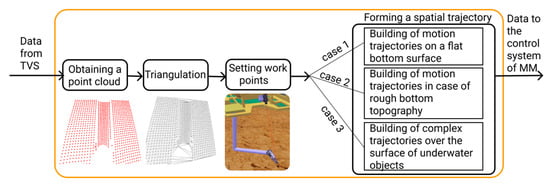
Figure 2.
The steps of the method.
Figure 3 shows a diagram of real-time supervisory control of MM 1 mounted on UUV 2 in the process of the sampling of a surface sediment layer using multibeam sonar 3. This sonar forms a point cloud to build a mathematical model of the seabed surface 4, which is used for the subsequent forming of the trajectory of the sediment sampler motion. The operator, moving the optical axis 5 of the camera, sets s target points (), which are the points of intersection of this axis with the bottom surface at the most interesting places for sediment sampling. The motion trajectory 6 of the sediment sampler is built automatically by connecting the points . Its vector during movement along the trajectory (see Figure 3) should always be perpendicular to the bottom surface, and the vector of the normal line to should be directed to the next target point .
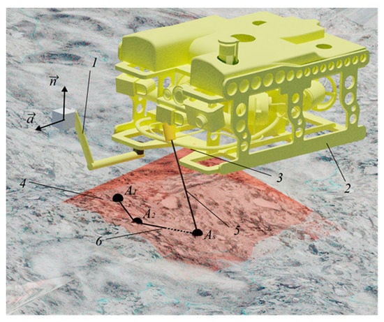
Figure 3.
An operation performed in the supervisory mode.
Similarly, the proposed method of supervisory control can be used to perform more complex manipulative operations, according to operator’s target indications.
3. Building of Motion Trajectories for a MM Working Tool Performing Operations on a Flat Bottom Surface
As numerous deep-sea studies [18,32] have shown, sampling of sediment layers and geological rocks is frequently carried out on a relatively flat seabed surface. Such a surface can be represented by an averaged plane [32]. To do this, it is sufficient to use point clouds of points obtained with a Doppler velocity log (DVL). A DVL has at least three hydroacoustic antennas and allows measurement of the distance from their location on the UUV hull to the bottom, along all the axes of these antennas with a high accuracy.
Therefore, in the coordinate system (CS) , rigidly fixed on the UUV hull, this plane can be described by the equation in the normal form [33]:
where , , and are the axes of the CS, with origin point O located at the UUV center of buoyancy; the axis coincides with the horizontal, longitudinal axis of the UUV; the axis coincides with its vertical axis; the y axis forms the right-hand triple with them; , , and are the directional cosines of the unit vector of the normal line to the plane (Equation (1)), which coincides with the vector ; and is the distance from the origin of the CS to this plane. The elements and are calculated using the cloud of points belonging to the bottom surface, formed by DVL, according to the method described in [32].
To form the motion trajectory of the MM working tool in the CS , it is necessary to calculate the coordinates of the target points (see Figure 3). If the camera is targeted at point , the position of this camera in the CS is determined by the preset point located on the optical axis, and its orientation is determined by the unit vector . In this case, the optical axis of the camera, coinciding with the vector that extends from the point towards the bottom plane (Equation (1)), is described by the following equation:
where is the parameter that varies within the limits . The value of the parameter at the point of intersection of the axis (Equation (2)) with the plane (Equation (1)) can be obtained by substituting Equation (2) in Equation (1) [34]:
The coordinates of the point at the intersection of the camera optical axis with the bottom plane are determined by substituting the found value of the parameter in Equation (2):
After the operator points the camera’s optical axis at the next target point , the value of the parameter is calculated using Equation (3) for the new point and vector . The coordinates of the rest of the target points are determined in the same way. As a result, the motion trajectory of the MM working tool is represented in the form of its sequential movements through all target points. The vector of the tool is always parallel to the vector , connecting the passed, and the next, target points.
4. Building of Motion Trajectories for a MM Working Tool in Case of Rough Bottom Topography
If the bottom surface has a rough topography, then it is necessary to use 3D multibeam sonars [35,36], which provide a high accuracy for formation of point clouds on the bottom surface in the area of the UUV operation. These clouds and other known methods are used [31,37] to build a triangulation model (see Figure 4), which is a multitude of triangular shapes stitched together. The trajectory of the MM working tool, passing through the target points set by the operator on the rough seabed surface, is formed on the basis of this model. Each kth triangle in the triangulation model is set in the CS as coordinates of three vertices , where and is the number of triangles.
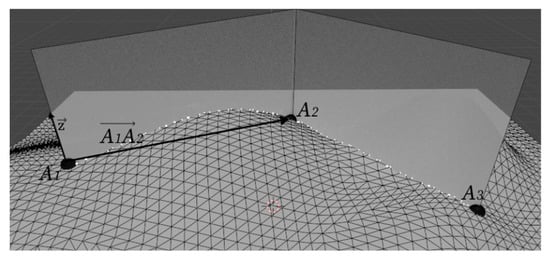
Figure 4.
A triangulation model of a seabed surface.
To find the coordinates of each target point at the intersection of the camera optical axis and the obtained triangulation surface in this CS, first, the triangle currently intersected by the axis (Equation (2)) should be found among all triangles. For this, the Möller–Trumbore algorithm [38] is used. Based on the coordinates of the point , the vector , and the vertices of all triangles, this algorithm identifies the kth triangle through which the axis (Equation (2)) passes. In this case, the coordinates of the point in the specified CS relative to the vertices of the kth triangle in vector form can be determined as follows:
where are the barycentric coordinates of the point relative to the vertices of the kth triangle ().
By expressing and substituting the equation of the axis (Equation (2)) in Equation (4), we obtain a system of equations with respect to the parameters :
which can be expressed in the matrix form:
Values of the parameters are obtained by solving Equation (5) [38]:
where () is the dot product of vectors, and () is the vector product of vectors.
The triangle k with the vertices , which intersects the axis (Equation (2)), is found with the following conditions [38]:
and the coordinates of the point of intersection of the camera optical axis with the kth triangle are determined by substituting the found parameter from Equation (6) in Equation (2):
For the subsequent building of the motion trajectory for the MM working tool passing through all the obtained points , this trajectory is represented as a sequence of transects of the triangulation surface, which are the vertical profiles of its parts between neighboring target points. These profiles can be represented as a set of points of intersection of the triangulation triangles sides and the plane formed by the vector , connecting neighboring target points, and the unit vector parallel to the axis in the CS (see Figure 4).
To build the motion trajectory for the MM working tool passing through the points of the triangles’ intersection with the plane formed by the vectors and , it is necessary to calculate which of all g triangles intersect the specified plane, and calculate the coordinates of the points of these intersections. When the fact that a side of the kth triangle intersects the specified plane has been established, the signs of the distances from the hth vertex (h = 0, 1, 2) to the plane formed by the vectors and are compared for each pair of its vertices by the algorithm [28]. The parameters are calculated by the formula , where is the vector connecting the target point with the hth vertex of the kth triangle.
If values of have the same signs ( and or and ) for any pair of the respective vertices of the kth triangle, then the plane does not intersect the kth triangle. If have different signs ( and or and ), then the point , through which the MM working tools should move, is lying on the side of the kth triangle formed by this pair of vertices (in general, the sides of each triangle can have no more than two points of intersection with the plane). The coordinates of the point for the side formed by the vertices and are determined by the formula [34]: , where is the vector connecting the vertices and of the kth triangle [34], and is the distance from the plane formed by the vectors and to the origin O of the CS .
The coordinates of the second point on one of the two remaining sides of the kth triangle, formed by the vertices and or and , are calculated in a similar way. If the equality is true, then the hth vertex of the kth triangle is lying on the specified plane. In this case, .
As a result, there is a set of points , through which the MM should move its working tool. Thus, at the points and , as well as during movement between these points, the vector is always perpendicular to the plane of the kth triangle, to which these points belong. Therefore, in the CS , the vector is always perpendicular to the plane defined by the three vertices of the kth triangle.
To build the desired trajectory of the working tool, the resulting set of points with their respective vectors are transformed into a sequence of points with vectors located between the adjacent target points and , where j is the sequential number of the point in the sequence of the working tool’s motion. In this case, the vector of this tool is always parallel to the vector connecting the passed, and the next, points of the set. As a result, the obtained sequence of points and their respective vectors and form the motion trajectory of the working tool (see Figure 5).
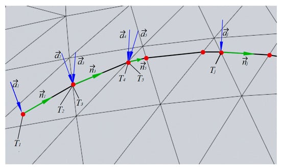
Figure 5.
A triangulation model of a seabed surface and the formed motion trajectory of the MM working tool.
5. Building of Complex Trajectories for MM Working Tools to Move Over the Surface of Underwater Objects
To perform complex manipulative operations, including those with subsea valve systems, cleaning silt and fouling, measurements of pipeline wall thickness, etc., the working tool of MM should move along complex spatial trajectories. The shape of such work objects is usually well known. Therefore, the desired motion trajectories of the MM can be built in advance, taking into account the requirements of certain technological operations. In this case, the operator can visually estimate the area of the underwater object on which the specified trajectory is to be overlaid. Using a video camera, the operator indicates the start and end points, with the desired trajectory between them automatically projected from the computer memory on the specified surface of the work object, taking into account the spatial position of this object [39].
When the UUV hovers over an object located in the scanning field of the TVS, the desired trajectory of the working tool can be immediately set in the CS of the UUV in the form of a sequence of points or in an analytical form. If this trajectory is set in the plane as a function , then it should be projected on the surface of the object in the direction of the unit vector that coincides with the negative direction of the axis of the CS . The operator targets the camera optical axis, setting the start and end points belonging to the object and determining the beginning and end of the working tool’s movement along the trajectory. The coordinates of these points are calculated using Equation (10).
To project the trajectory on a sector of the object’s triangulation surface confined between the points and , this trajectory, set in analytical form, is first converted into a sequence of auxiliary points For this, the coordinates of the points are calculated as follows:
where is the confirmed value of the y coordinate from x obtained by the analytical expression , ; g is the step along the x axis, which determines the number of auxiliary points (determined by the parameters of this trajectory and the degree of detail of the scanned object). An increase in the number of points enhances the accuracy of the trajectory formation but requires an increase in the number of calculations. To take into account the spatial position and orientation of certain areas of the work objects when projecting points , first, all the vectors connecting the origin O of the CS with the points should be rotated at an angle around the axis. Then the second rotation should be performed around the axis of the CS at an angle confined between the vector and the plane . Afterwards, a linear transfer of the obtained vectors is performed along the x and y axes by the values and , respectively. As a result, the coordinates of the sought points will be determined using the following equation:
where and are the matrices of elementary rotations around the and axes of the CS , respectively, and is the matrix of complex rotation [40].
The intersections of the projection rays extending from the points in the direction of the vector with the triangulation surface model form a sequence of points (see Figure 6). The sequence of these points describes the desired motion trajectory of the working tool, located between the points indicated by the operator.
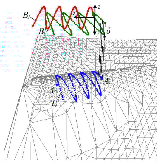
Figure 6.
The desired trajectory overlaid on the surface of the underwater object.
The coordinates of the points are determined using the Möller–Trumbore algorithm [38] with Equation (11) taken into account in the following form:
The vectors and , corresponding to each point , are calculated using the algorithm described in Section 3. To find the point , it is necessary to determine the intersections of each triangle in the triangulation grid by the ray extending from the point . In case of a large number of projecting rays or triangles, the search for the intersections of each triangle by each ray (starting from the first one) requires a lot of computational resources. To reduce the number of necessary computational operations (including false ones, where the selected triangle has no intersection points with a certain ray), when searching for the point , first, a test is carried out to check if the ray extending from the point intersects the triangle where the point is located. If there is no intersection, then the search for the intersected triangle begins in the normal mode, starting from the first one.
6. Software Implementation and Results of the Study of the Method for Supervisory Control of an MM Mounted on a UUV
The developed method for supervisory control of an MM was implemented in the C++ programming language. The input data for the created program is a set of points on the underwater object surface, obtained using TVS and fixed in 3D space. The coordinates of the points and vectors , specified by the operator, that define the position of the camera optical axis in the CS are input in the same program.
The created program allows building triangulation models for surfaces of underwater objects using the algorithm [31]. After the operator specifies the points and vectors , the coordinates of the target points and the sequence of points (see Figure 5 and Figure 6) and their respective vectors and are calculated for a certain MM working tool using this program implementation.
For a more precise description of the underwater objects’ shape, and also for the subsequent control of the formation of MM motion trajectories, a graphical interface was created using the OpenGL Core libraries (see Figure 7), which displays the triangulation surface of the object being observed, the trajectory projected on this surface, and the video image coming from the camera in real-time mode. Using the resulting image, the operator can check the correct construction of the automatically generated trajectory before starting a manipulative operation.
Figure 7.
Interface for controlling the formation of motion trajectories of the MM working tool.
Since the method is based on spatial geometric transformations (finding intersections of the camera’s optical axis with the triangulation surface and with the subsequent projection of the desired trajectories on this surface), its accuracy depends only on the accuracy of point clouds obtained from the TVS and on the features of the triangulation algorithms used for these points. Therefore, the method can easily be implemented both in systems for semi-natural modeling and testing [41] and for an actual UUV, regardless of the kinematic and dynamic features of these vehicles and their MM.
The proposed method was tested by numerical simulation in the V-REP environment. A scenario of one of the manipulative operations for cleaning a continuous pipeline from fouling is shown in Figure 8a. A model of multibeam sonar with a resolution of 32 × 32 dots and a unidirectional scanning pattern was used as the TVS. The sequence of points and their respective vectors and of the MM working tool, formed by the program, was transferred to the Matlab/Simulink via the UDP protocol. In Matlab/Simulink, the resulting sequence was smoothed using a third-order parametric B-spline [42]. Program control signals for the electric drives of the respective degrees of MM mobility were generated using this sequence. During the simulation, we used a well-tested mathematical model of a UUV [43] with a mounted MM based on the PUMA kinematic model, which has the first five degrees of freedom (3 translatory and 2 orientation). The main parameters of the UUV and its MM are given in Table 1. All parameters of the kinematic and dynamic model of the UUV are provided in [44,45]. The mathematical model of the underwater MM used and its parameters are described in detail in [46]. This model includes a recurrent algorithm for solving the inverse dynamics problem, which takes into account not only the joint coupling between degrees of mobility of the MM, but also the effects of a viscous environment on its moving links, as well as the experimentally determined parameters of these effects [47]. To stabilize the UUV in the hovering mode, a combined system [21,48] was used, which makes it possible to compensate for the impacts of marine currents and the dynamic impacts from moving the MM, calculated in real time, with the UUV thrusters.
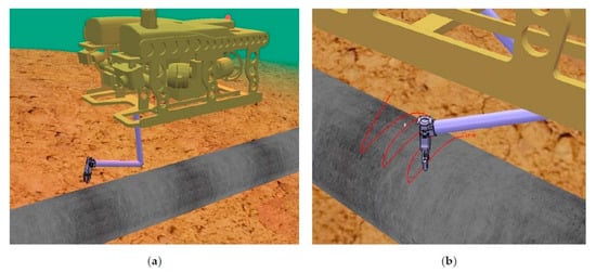
Figure 8.
(a) A model of the UUV, MM, and work object in V-REP; (b) a formed motion trajectory of the MM working tool in V-REP.

Table 1.
Parameters of the UUV and MM.
To visualize the MM motions over the surface of work objects, the data (generalized coordinates of MM, and linear and angular displacements of the UUV relative to the initial point of its stabilized positioning) obtained during the simulation of the complex dynamic model of the UUV with MM were sent from Matlab/Simulink back to V-REP by the UDP protocol. The results of the visualization of the actual technological manipulative operation performed are shown in Figure 8a,b.
An assessment of the relative positions of the pipeline surface and the MM working tool was made using Figure 8b. On the basis of the analysis carried out, it became possible to automatically generate and then, using the proposed method, pass through the complex motion trajectories, thus, precisely performing quite complex manipulative operations with the working tool. The operator gave only the target indications and checked the correctness of the working tool’s automatically built motion trajectories along the surface of the work object by means of the designed graphical interface. This greatly simplified and facilitated the operator’s work. Implementation of the program tools for the proposed method should not pose any serious difficulties, since these tools do not have significant computational complexity and can be installed on standard on-board computers.
7. Conclusions
In the present study, we addressed the problem of developing a new method for supervisory control of complex manipulative operations, which can significantly increase the speed and simplify complex work and operations by automating the entire technological process, while reducing the mental load on the MM operator. A significant increase in the efficiency of manipulative operations was achieved by precisely building complex curved trajectories of the MM working tool’s motion on the basis of operator target indications. The trajectories built are accurately performed by the MM with the required orientation of the working tools in an automatic mode. The operator, by targeting the optical axis of the video camera mounted on the UUV rotary platform, sets the start and end points of the motion trajectories for these tools and the boundaries of specified areas of the work objects. Then the trajectories, formed by taking into account the shape and spatial position of the work areas, are projected onto them.
The developed method of supervisory control was implemented in the C++ programming language. The specifics of application of the method have been tested through numerical simulation in the V-REP environment. A graphical interface has been created that provides rapid testing of the accuracy of overlaying the planned trajectories on the mathematically described surface of the work object. The results of the simulation of actual technological operations with the use of an MM mounted on a UUV confirmed the high efficiency of the proposed method and the simplicity of its practical application.
Further work will focus on creating methods and algorithms for intellectual support of operators’ activities during implementation of supervisory control modes for UUV with MM, while taking into account the limited bandwidth of hydroacoustic communication channels. Herewith, the issues of providing a dialog mode for MM control will be ad-dressed, factors and conditions that could potentially cause emergency situations identified, and timely measures to prevent them taken by generating warnings and recommendations for UUV operators.
Author Contributions
Conceptualization and methodology, A.K.; software, A.Y.; formal analysis, A.K., V.F. and A.Y.; investigation, A.Y.; writing—original draft preparation, A.K. and A.Y.; writing—review and editing, A.K., V.F. and A.Y.; visualization, A.Y.; project administration, validation, supervision and funding acquisition, A.K. All authors have read and agreed to the published version of the manuscript.
Funding
This research was funded by the Ministry of Science and Higher Education of the Russian Federation, grant number 13.1902.21.0012 “Fundamental Problems of Study and Conservation of Deep-Sea Ecosystems in Potentially Ore-Bearing Areas of the Northwestern Pacific” (agreement no. 075-15-2020-796)”.
Institutional Review Board Statement
Not applicable.
Informed Consent Statement
Not applicable.
Data Availability Statement
Request to corresponding author of this article.
Conflicts of Interest
The authors declare no conflict of interest.
References
- Davey, V.S.; Forli, O.; Raine, G.; Whillock, R. Non-Destructive Examination of Underwater Welded Steel Structures; Woodhead Publishing: Cambridge, UK, 1999; Volume 1372, p. 75. [Google Scholar]
- Gracias, N.; Negahdaripour, S. Underwater Mosaic Creation using Video sequences from Different Altitudes. In Proceedings of the OCEANS 2005 MTS/IEEE, Washington, DC, USA, 18–23 September 2006; pp. 1295–1300. [Google Scholar] [CrossRef]
- Christ, R.; Wernli, R. The ROV Manual: A User Guide for Remotely Operated Vehicles, 2nd ed.; Elsevier Science: Oxford, UK, 2013; p. 667. [Google Scholar]
- Carrera, A.; Ahmadzadeh, S.R.; Ajoudani, A.; Kormushev, P.; Carreras, M.; Caldwell, D.G. Towards Autonomous Robotic Valve Turning. Cybern. Inf. Technol. 2012, 12, 17–26. [Google Scholar] [CrossRef]
- Di Lillo, P.; Simetti, E.; Wanderlingh, F.; Casalino, G.; Antonelli, G. Underwater Intervention with Remote Supervision via Satellite Communication: Developed Control Architecture and Experimental Results Within the Dexrov Project. IEEE Trans. Control. Syst. Technol. 2021, 29, 108–123. [Google Scholar] [CrossRef]
- Noé, S.; Beck, T.; Foubert, A.; Grehan, A. Surface Samples in Belgica Mound Province Hovland Mound Province, West Rockall Bank and Northern Porcupine Bank. In Shipboard Party: Report and Preliminary Results of RV Meteor Cruise M61/3; Ratmeyer, V., Hebbeln, D., Eds.; Universität Bremen: Bremen, Germany, 2006; pp. 28–32. [Google Scholar]
- Galloway, K.C.; Becker, K.P.; Phillips, B.; Kirby, J.; Licht, S.; Tchernov, D.; Wood, R.J.; Gruber, D.F. Soft Robotic Grippers for Biological Sampling on Deep Reefs. Soft Robot. 2016, 3, 23–33. [Google Scholar] [CrossRef]
- Di Vito, D.; De Palma, D.; Simetti, E.; Indiveri, G.; Antonelli, G. Experimental validation of the modeling and control of a multibody underwater vehicle manipulator system for sea mining exploration. J. Field Robot. 2021, 38, 171–191. [Google Scholar] [CrossRef]
- Coleman, D.F.; Ballard, R.D.; Gregory, T. Marine archaeological exploration of the black sea. In Oceans 2003 Celebrating the Past... Teaming toward the Future; IEEE: New York, NY, USA, 2003; Volume 3, pp. 1287–1291. [Google Scholar] [CrossRef]
- Hachicha, S.; Zaoui, C.; Dallagi, H.; Nejim, S.; Maalej, A. Innovative design of an underwater cleaning robot with a two arm manipulator for hull cleaning. Ocean Eng. 2019, 181, 303–313. [Google Scholar] [CrossRef]
- Peñalver, A.; Pérez, J.; Fernández, J.; Sales, J.; Sanz, P.; García, D.F.; Fornas, D.; Marín, R. Visually-guided manipulation techniques for robotic autonomous underwater panel interventions. Annu. Rev. Control. 2015, 40, 201–211. [Google Scholar] [CrossRef][Green Version]
- Filaretov, V.; Konoplin, A. System of Automatically Correction of Program Trajectory of Motion of Multilink Manipulator Installed on Underwater Vehicle. Procedia Eng. 2015, 100, 1441–1449. [Google Scholar] [CrossRef][Green Version]
- Antonelli, G.; Caccavale, F.; Chiaverini, S. Adaptive Tracking Control of Underwater Vehicle-Manipulator Systems Based on the Virtual Decomposition Approach. IEEE Trans. Robot. Autom. 2004, 20, 594–602. [Google Scholar] [CrossRef]
- Mohan, S.; Kim, J. Coordinated motion control in task space of an autonomous underwater vehicle–manipulator system. Ocean Eng. 2015, 104, 155–167. [Google Scholar] [CrossRef]
- Zhang, J.; Li, W.; Yu, J.; Feng, X.; Zhang, Q.; Chen, G. Study of manipulator operations maneuvered by a ROV in virtual environments. Ocean Eng. 2017, 142, 292–302. [Google Scholar] [CrossRef]
- Bin Ambar, R.; Sagara, S. Development of a master controller for a 3-link dual-arm underwater robot. Artif. Life Robot. 2015, 20, 327–335. [Google Scholar] [CrossRef]
- Sakagami, N.; Shibata, M.; Hashizume, H.; Hagiwara, Y.; Ishimaru, K.; Ueda, T.; Saitou, T.; Fujita, K.; Kawamura, S.; Inoue, T.; et al. Development of a human-sized ROV with dual-arm. In OCEANS’10 IEEE SYDNEY; IEEE: New York, NY, USA, 2010; pp. 1–6. [Google Scholar] [CrossRef]
- Galkin, S.V.; Vinogradov, G.M.; Tabachnik, K.M.; Rybakova, E.I.; Konoplin, A.Y.; Ivin, V.V. Megafauna of the Bering Sea Slope Based on Observations and Imaging from ROV “Comanche”; Marine Imaging Workshop: Kiel, Germany, 2017. [Google Scholar]
- Konoplin, A.Y.; Konoplin, N.Y.; Filaretov, V. Development of Intellectual Support System for ROV Operators. In IOP Conference Series: Earth and Environmental Science; IOP Publishing: Bristol, UK, 2019; Volume 272, p. 032101. [Google Scholar]
- Filaretov, V.F.; Konoplin, N.Y.; Konoplin, A.Y. Approach to Creation of Information Control System of Underwater Vehicles. In Proceedings of the IEEE 2017 International Conference on Industrial Engineering, Applications and Manufacturing (ICIEAM), St. Petersburg, Russia, 16–19 May 2017; pp. 1–5. [Google Scholar]
- Filaretov, V.; Konoplin, A.Y. System of automatic stabilization of underwater vehicle in hang mode with working multilink manipulator. In Proceedings of the 2015 International Conference on Computer, Control, Informatics and its Applications (IC3INA); Institute of Electrical and Electronics Engineers (IEEE), Bandung, Indonesia, 5–7 October 2015; pp. 132–137. [Google Scholar]
- Vu, M.T.; Le, T.-H.; Thanh, H.L.N.N.; Huynh, T.-T.; Van, M.; Hoang, Q.-D.; Do, T.D. Robust Position Control of an Over-actuated Underwater Vehicle under Model Uncertainties and Ocean Current Effects Using Dynamic Sliding Mode Surface and Optimal Allocation Control. Sensors 2021, 21, 747. [Google Scholar] [CrossRef] [PubMed]
- Vu, M.T.; Le Thanh, H.N.N.; Huynh, T.T.; Thang, Q.; Duc, T.; Hoang, Q.D.; Le, T.H. Station-keeping control of a hovering over-actuated autonomous underwater vehicle under ocean current effects and model uncertainties in horizontal plane. IEEE Access 2021, 9, 6855–6867. [Google Scholar] [CrossRef]
- Kang, J.I.; Choi, H.S.; Vu, M.T.; Duc, N.N.; Ji, D.H.; Kim, J.Y. Experimental study of dynamic stability of underwater vehicle-manipulator system using zero moment point. J. Mar. Sci. Technol. 2017, 25, 767–774. [Google Scholar] [CrossRef]
- Yoerger, D.R.; Slotine, J.-J.E. Supervisory control architecture for underwater teleoperation. In Proceedings of the 1987 IEEE International Conference on Robotics and Automation; Institute of Electrical and Electronics Engineers (IEEE), Berkeley, CA, USA, April 2005; Volume 4, pp. 2068–2073. [Google Scholar]
- Yoerger, D.; Newman, J.; Slotine, J.-J. Supervisory control system for the JASON ROV. IEEE J. Ocean. Eng. 1986, 11, 392–400. [Google Scholar] [CrossRef]
- Zhang, J.; Li, W.; Yu, J.; Mao, X.; Li, M.; Chen, G. Operating an underwater manipulator via P300 brainwaves. In Proceedings of the 2016 23rd International Conference on Mechatronics and Machine Vision in Practice (M2VIP); Institute of Electrical and Electronics Engineers (IEEE), Nanjing, China, 28–30 November 2016; pp. 1–5. [Google Scholar]
- Sivčev, S.; Rossi, M.; Coleman, J.; Dooly, G.; Omerdic, E.; Toal, D. Fully automatic visual servoing control for work-class marine intervention ROVs. Control. Eng. Pr. 2018, 74, 153–167. [Google Scholar] [CrossRef]
- Bruno, F.; Lagudi, A.; Barbieri, L.; Rizzo, D.; Muzzupappa, M.; De Napoli, L. Augmented reality visualization of scene depth for aiding ROV pilots in underwater manipulation. Ocean Eng. 2018, 168, 140–154. [Google Scholar] [CrossRef]
- Joe, H.; Kim, J.; Yu, S.-C. Sensor Fusion-based 3D Reconstruction by Two Sonar Devices for Seabed Mapping. IFAC-PapersOnLine 2019, 52, 169–174. [Google Scholar] [CrossRef]
- Marton, Z.C.; Rusu, R.B.; Beetz, M. On fast surface reconstruction methods for large and noisy point clouds. In Proceedings of the 2009 IEEE International Conference on Robotics and Automation; Institute of Electrical and Electronics Engineers (IEEE), Kobe, Japan, 12–17 May 2009; pp. 3218–3223. [Google Scholar]
- Filaretov, V.F.; Konoplin, A.Y.; Konoplin, N.Y. System for automatic soil sampling by AUV equipped with multilink manipulator. Int. J. Energy Technol. Policy 2019, 15, 208. [Google Scholar] [CrossRef]
- Korn, G.A.; Korn, T.M. Mathematical handbook for scientists and engineers: Definitions, theorems, and formulas for reference and review. In Courier Corporation; Dover Publication, Inc.: Mineola, NY, USA, 24 June 2000; p. 1097. [Google Scholar]
- Schneider, P.J.; Eberly, D.H. Geometric Tools for Computer Graphics; Elsevier BV: Amsterdam, The Netherlands, 2003; p. 946. [Google Scholar]
- Tritech Eclipse. Multibeam Sonar for 3D Model View of Sonar Imagery. Available online: http://www.tritech.co.uk/ (accessed on 1 June 2021).
- BlueView 3D Multibeam Scanning Sonar. Available online: http://www.teledynemarine.com/ (accessed on 1 June 2021).
- Point Cloud Library: Fast Triangulation of Unordered Point Clouds. Available online: http://ns50.pointclouds.org/ (accessed on 1 June 2021).
- Möller, T.; Trumbore, B. Fast, Minimum Storage Ray-Triangle Intersection. J. Graph. Tools 1997, 2, 21–28. [Google Scholar] [CrossRef]
- Konoplin, A.Y.; Konoplin, N.Y.; Shuvalov, B.V. Technology for Implementation of Manipulation Operations with Different Underwater Objects by AUV. In Proceedings of the 2019 International Conference on Industrial Engineering, Applications and Manufacturing (ICIEAM); Institute of Electrical and Electronics Engineers (IEEE), Sochi, Russia, 25–28 March 2019; pp. 1–5. [Google Scholar]
- Craig, J.J. Introduction to Robotics: Mechanics and Control; Pearson Prentice Hall: Upper Saddle River, NJ, USA, 2005; Volume 3. [Google Scholar]
- Fromm, T.; Mueller, C.A.; Pfingsthorn, M.; Birk, A.; Di Lillo, P. Efficient continuous system integration and validation for deep-sea robotics applications. In OCEANS 2017-Aberdeen; IEEE: New York, NY, USA, 2017; pp. 1–6. [Google Scholar] [CrossRef]
- Filaretov, V.; Gubankov, A.; Gornostaev, I. The formation of motion laws for mechatronics objects along the paths with the desired speed. In Proceedings of the 2016 International Conference on Computer, Control, Informatics and its Applications (IC3INA); Institute of Electrical and Electronics Engineers (IEEE), Jakarta, Indonesia, 3–5 October 2016; pp. 93–96. [Google Scholar]
- Fossen, T.I. Handbook of Marine Craft Hydrodynamics and Motion Control; John Wiley & Sons: Hoboken, NJ, USA, 2011; p. 736. [Google Scholar]
- Herman, P. Numerical Test of Several Controllers for Underactuated Underwater Vehicles. Appl. Sci. 2020, 10, 8292. [Google Scholar] [CrossRef]
- Vervoort, J. Modeling and Control of an Unmanned Underwater Vehicle. Ph.D. Thesis, Christchurch, New Zealand, 2009; pp. 5–15. [Google Scholar]
- Filaretov, V.F.; Konoplin, A.; Zuev, A.; Krasavin, N. System of High-precision Movements Control of Underwater Manipulator. In Proceedings of the 29th International DAAAM Symposium 2018, Zadar, Croatia, 24–27 October 2020; Volume 7, pp. 752–757. [Google Scholar] [CrossRef]
- Filaretov, V.; Konoplin, A. Experimental Definition of the Viscous Friction Coefficients for Moving Links of Multilink Underwater Manipulator. In Proceedings of the 29th International DAAAM Symposium 2018; DAAAM International, Zadar, Croatia, 24–27 October 2016; Volume 1, pp. 762–767. [Google Scholar]
- Filaretov, V.; Konoplin, A.Y. Development of control systems for implementation of manipulative operations in hovering mode of underwater vehicle. In OCEANS 2016-Shanghai; IEEE: New York, NY, USA, 2016; pp. 1–5. [Google Scholar] [CrossRef]
Publisher’s Note: MDPI stays neutral with regard to jurisdictional claims in published maps and institutional affiliations. |
© 2021 by the authors. Licensee MDPI, Basel, Switzerland. This article is an open access article distributed under the terms and conditions of the Creative Commons Attribution (CC BY) license (https://creativecommons.org/licenses/by/4.0/).