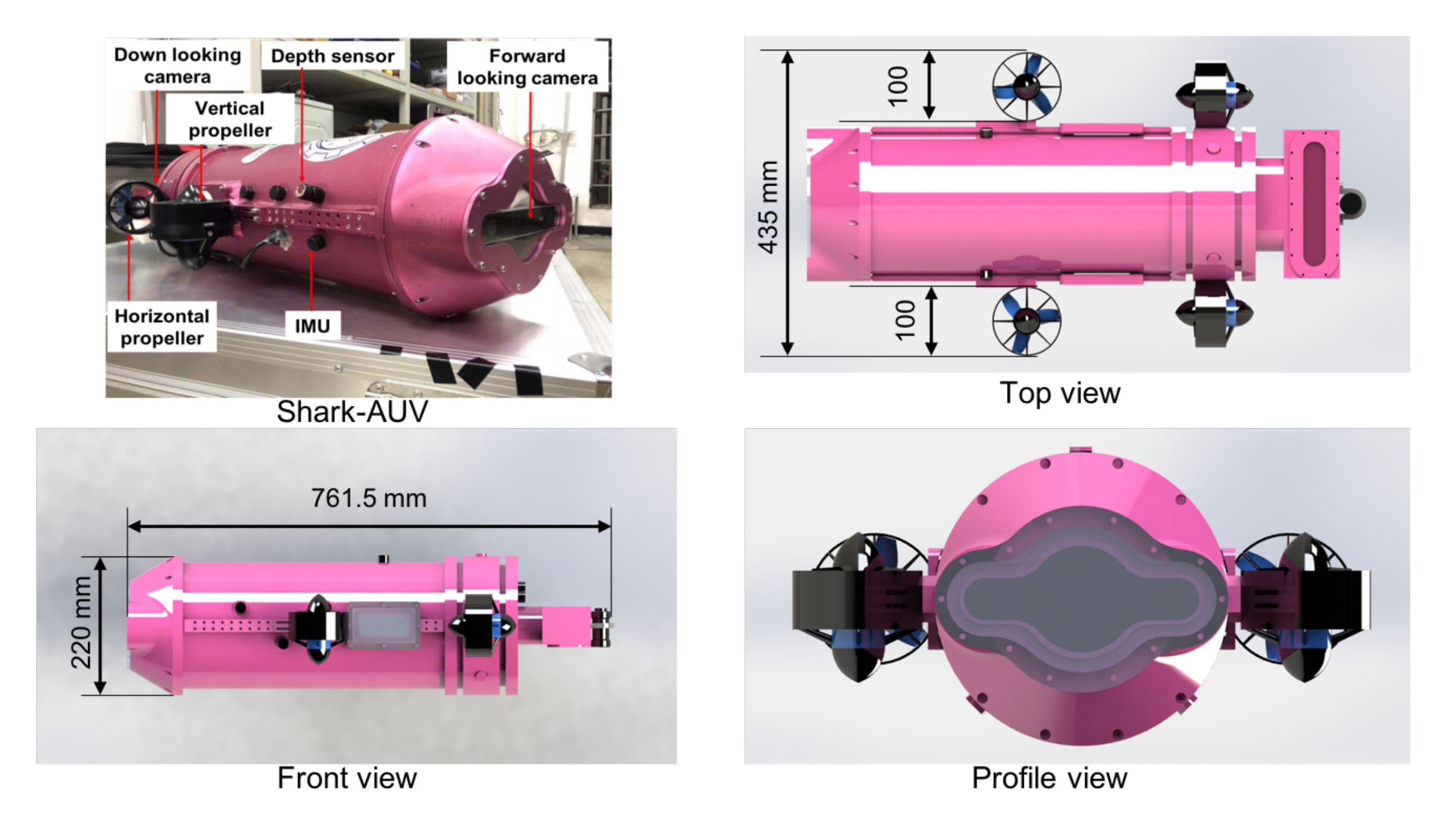
Figure 1.
Mechanical structure and configuration of the Shark-AUV.
Figure 1.
Mechanical structure and configuration of the Shark-AUV.
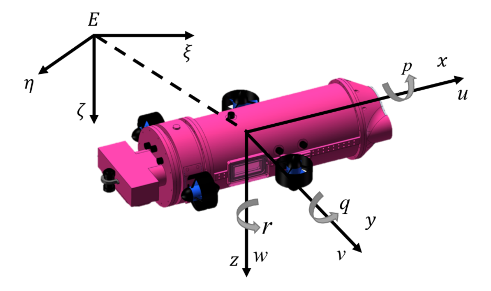
Figure 2.
Coordinate frame of the Shark-AUV.
Figure 2.
Coordinate frame of the Shark-AUV.
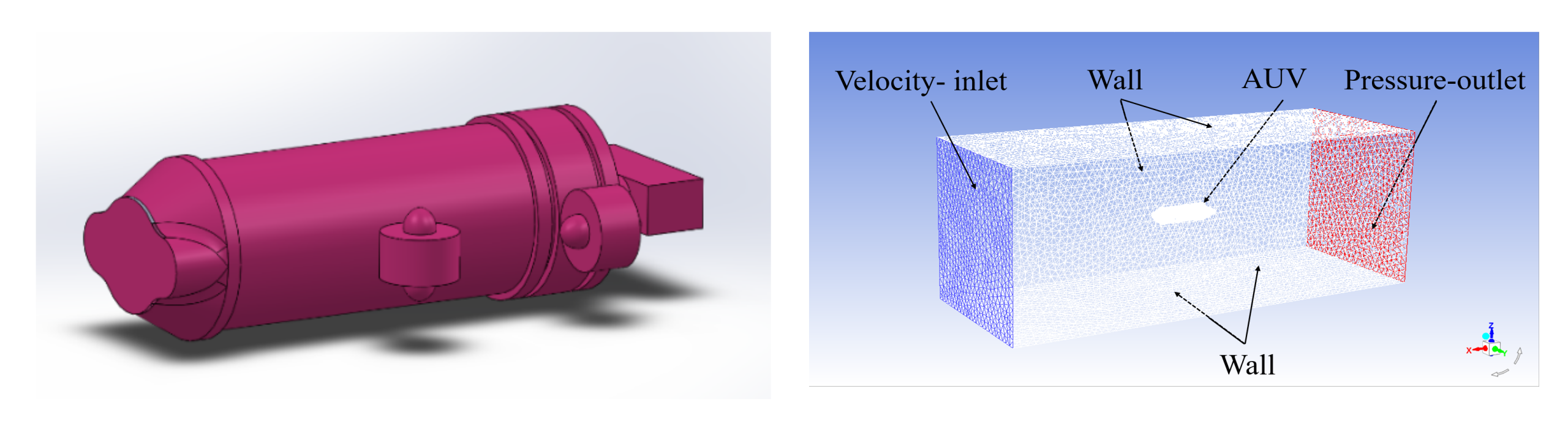
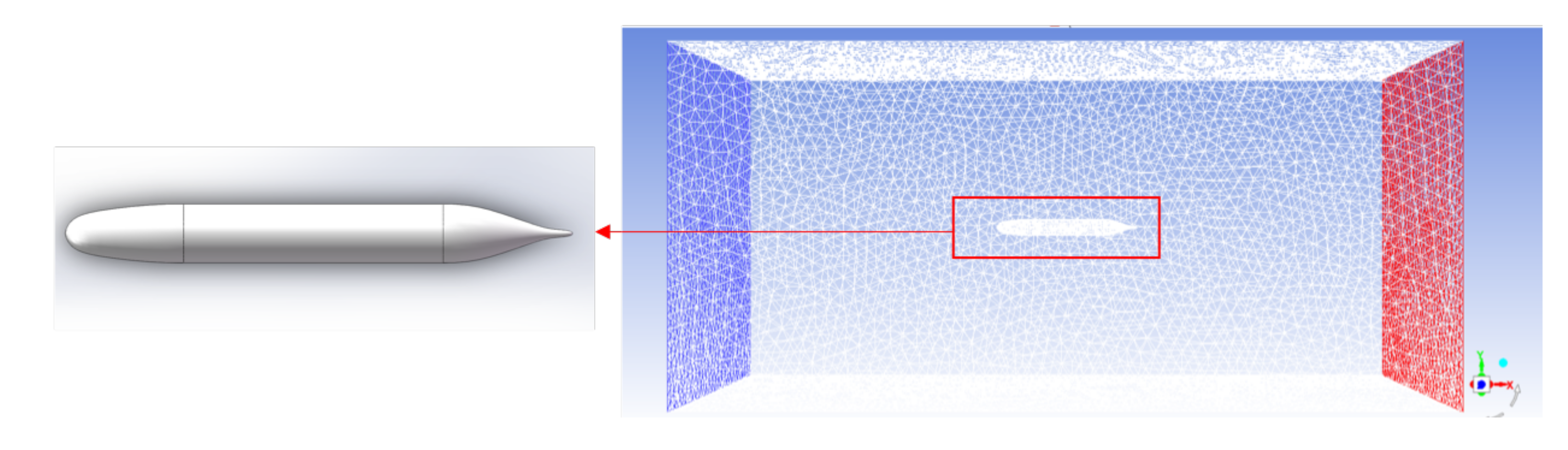
Figure 3.
Left diagram shows the full-scale 3D model of the Shark-AUV; the right one shows the computational domain of the CFD simulation.
Figure 3.
Left diagram shows the full-scale 3D model of the Shark-AUV; the right one shows the computational domain of the CFD simulation.
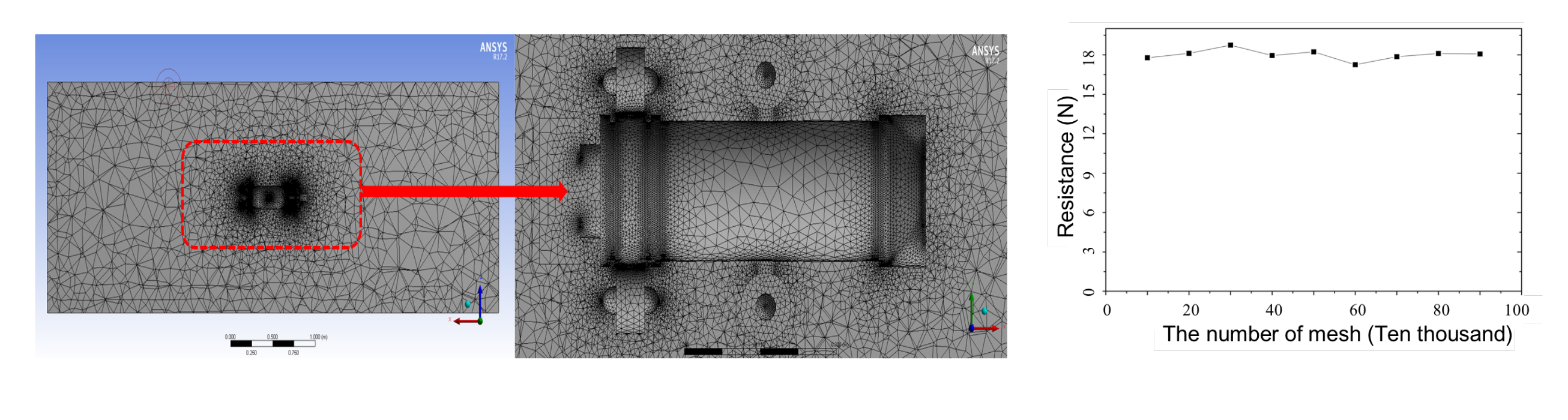
Figure 4.
Left diagram shows meshing of the 3D model of the Shark-AUV; the right one shows the resistance of the AUV versus the number of meshes.
Figure 4.
Left diagram shows meshing of the 3D model of the Shark-AUV; the right one shows the resistance of the AUV versus the number of meshes.
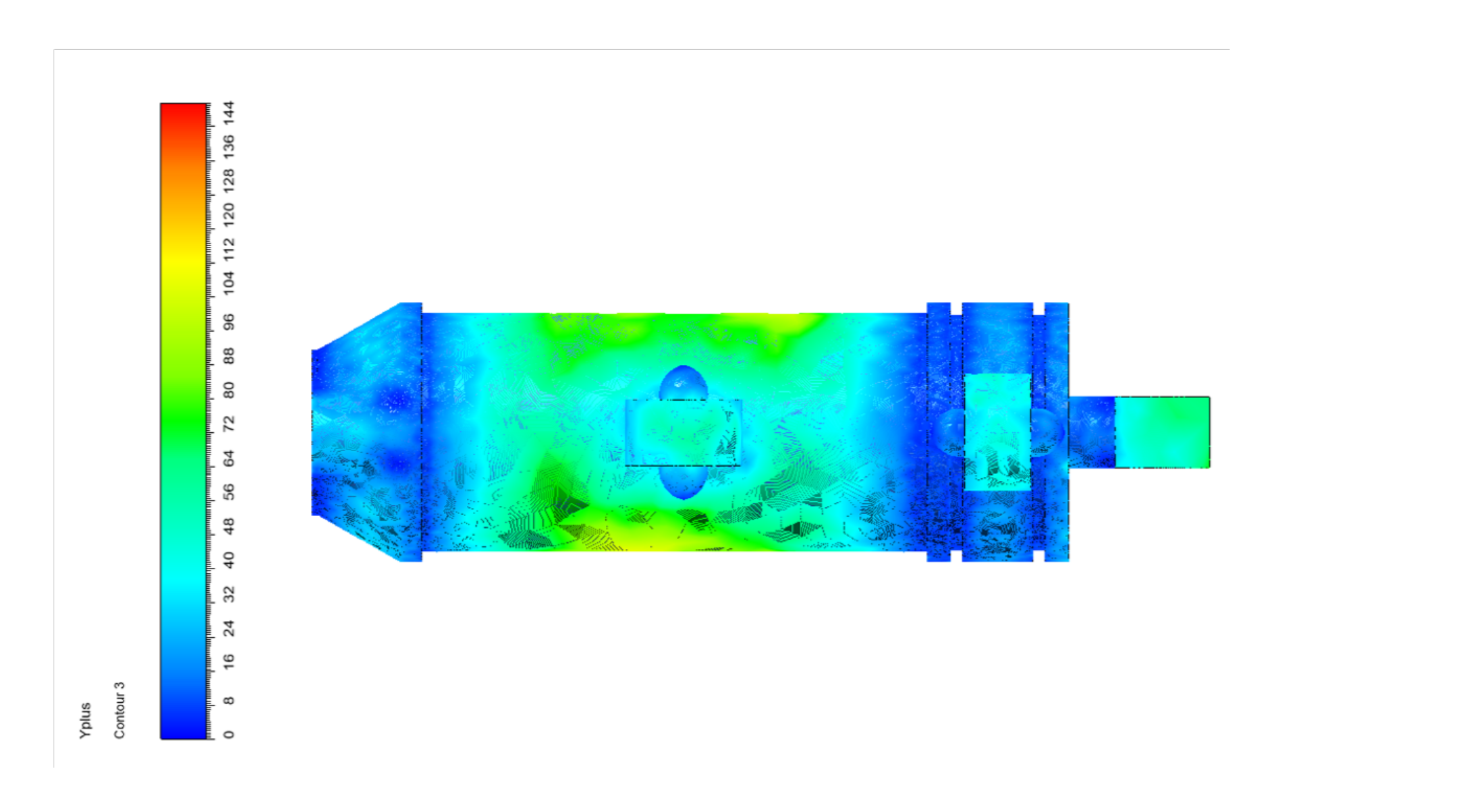
Figure 5.
value when the Shark-AUV cruises along the -direction at 0.5 m/s.
Figure 5.
value when the Shark-AUV cruises along the -direction at 0.5 m/s.
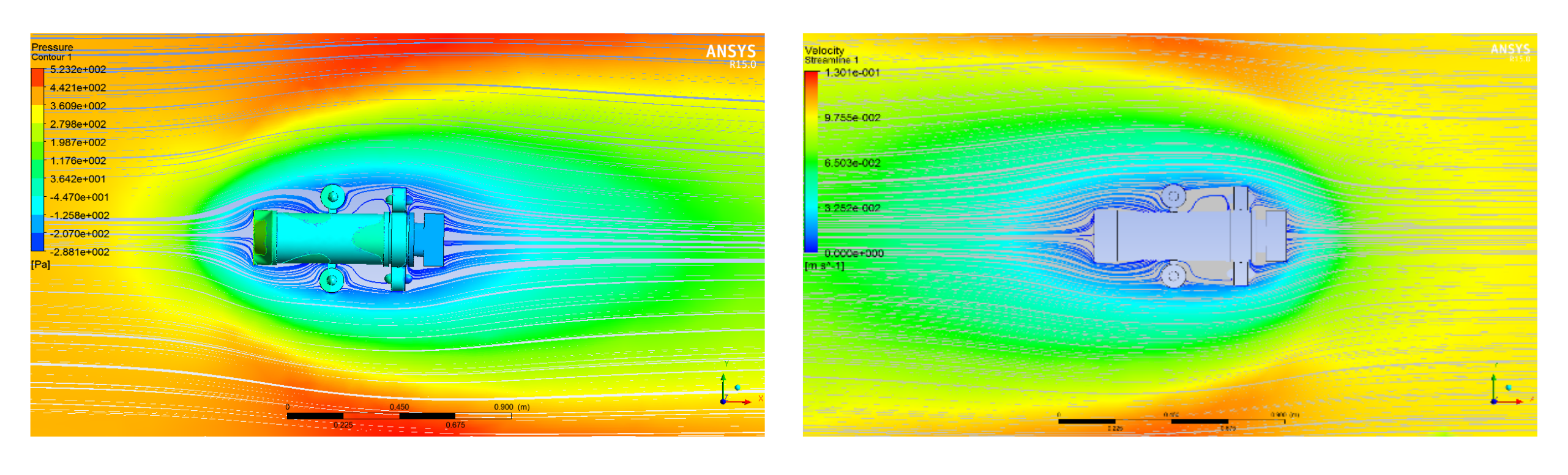
Figure 6.
Left diagram shows the flow around Shark-AUV cruising along -direction; the right one shows flow around Shark-AUV cruising along -direction.
Figure 6.
Left diagram shows the flow around Shark-AUV cruising along -direction; the right one shows flow around Shark-AUV cruising along -direction.
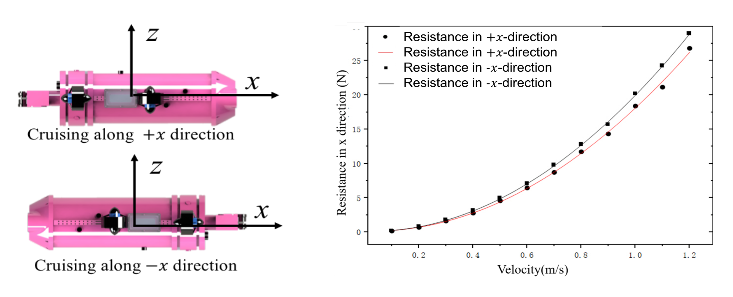
Figure 7.
Left diagram shows the Shark-AUV cruising along -directions in a body reference frame; the right one shows the curves of hydrodynamic resistances versus velocity of the AUV cruising along -directions.
Figure 7.
Left diagram shows the Shark-AUV cruising along -directions in a body reference frame; the right one shows the curves of hydrodynamic resistances versus velocity of the AUV cruising along -directions.
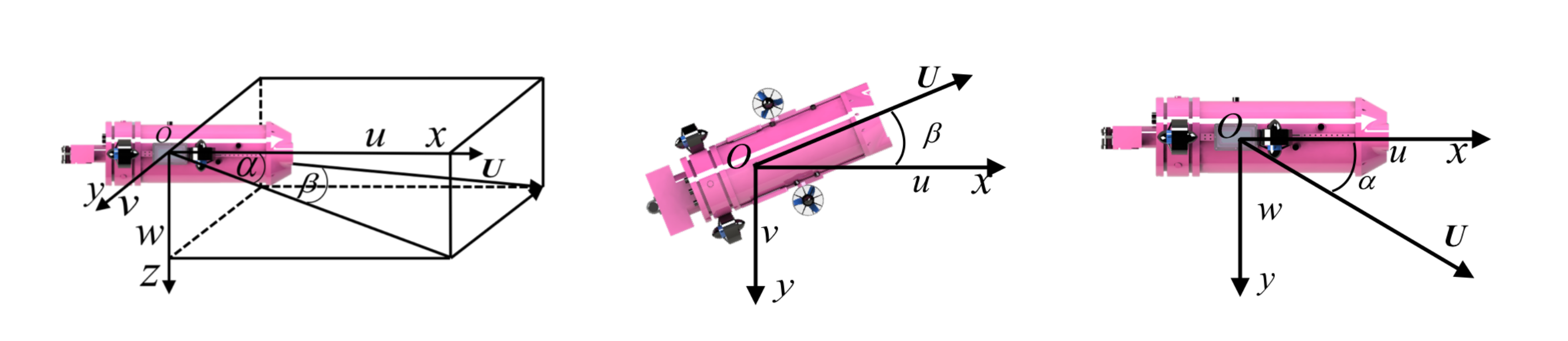
Figure 8.
Left diagram shows hydrodynamic angles of the Shark-AUV; the middle diagram shows the oblique motion of the AUV in the horizontal plane; the right diagram shows the oblique motion of the AUV in the vertical plane.
Figure 8.
Left diagram shows hydrodynamic angles of the Shark-AUV; the middle diagram shows the oblique motion of the AUV in the horizontal plane; the right diagram shows the oblique motion of the AUV in the vertical plane.
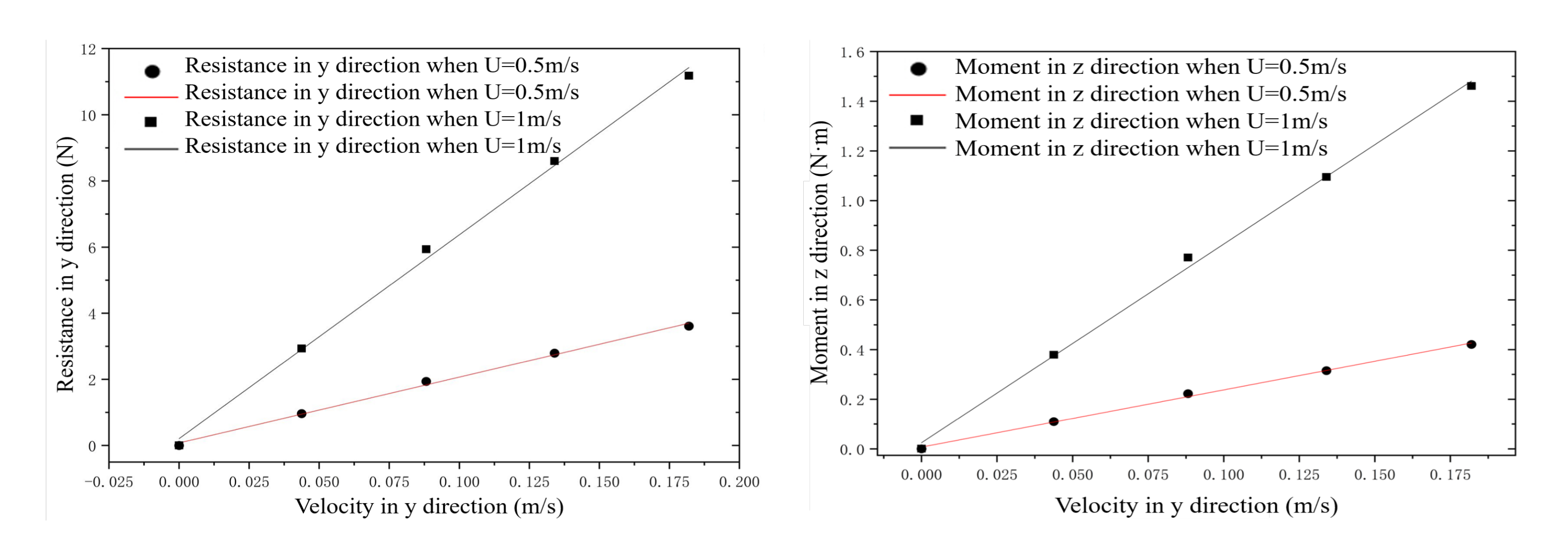
Figure 9.
Left diagram shows the relationship of lateral resistance Y versus lateral velocity v; the right diagram shows the relationship of roll moments N versus lateral velocity v.
Figure 9.
Left diagram shows the relationship of lateral resistance Y versus lateral velocity v; the right diagram shows the relationship of roll moments N versus lateral velocity v.
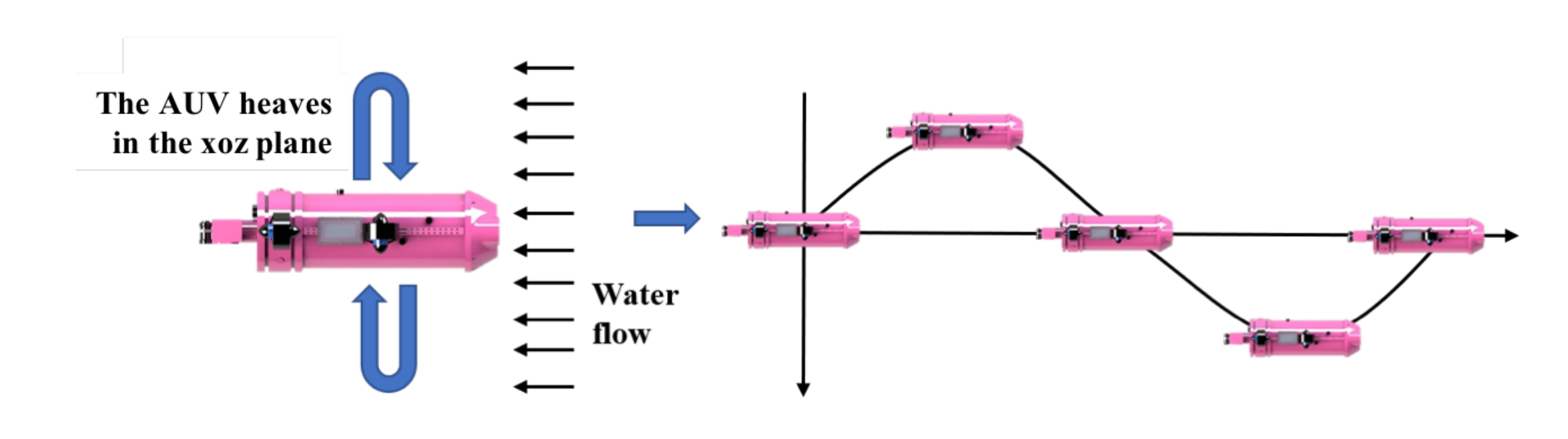
Figure 10.
Schematic diagram of heave motion of the Shark-AUV.
Figure 10.
Schematic diagram of heave motion of the Shark-AUV.
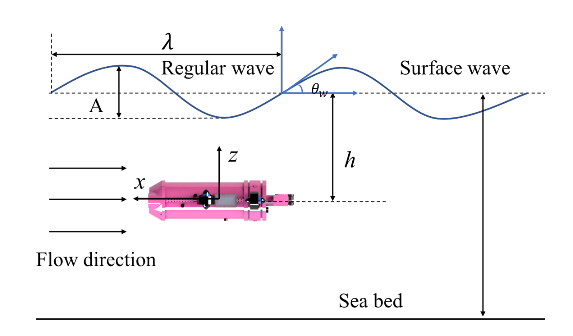
Figure 11.
Schematic diagram of the Sharks-AUV subjected to surface waves.
Figure 11.
Schematic diagram of the Sharks-AUV subjected to surface waves.
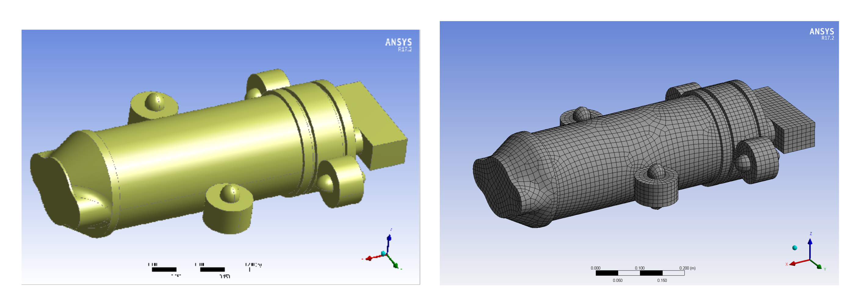
Figure 12.
Panel model of the Shark-AUV and meshing of the model.
Figure 12.
Panel model of the Shark-AUV and meshing of the model.
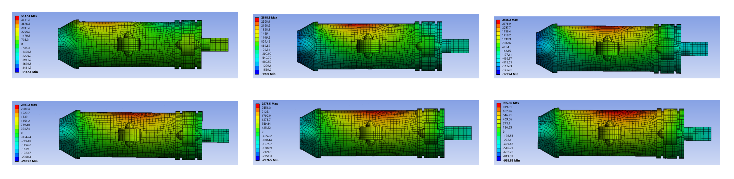
Figure 13.
From top to bottom, from left to right: surface pressure nephogram of the Shark-AUV at different submerged depths (h = 0.6 d, 0.7 d, 0.8 d, 0.9 d, 1 d, 2 d) when the AUV moves in a head wave and is located in the trough with a wave amplitude of 0.4 m.
Figure 13.
From top to bottom, from left to right: surface pressure nephogram of the Shark-AUV at different submerged depths (h = 0.6 d, 0.7 d, 0.8 d, 0.9 d, 1 d, 2 d) when the AUV moves in a head wave and is located in the trough with a wave amplitude of 0.4 m.
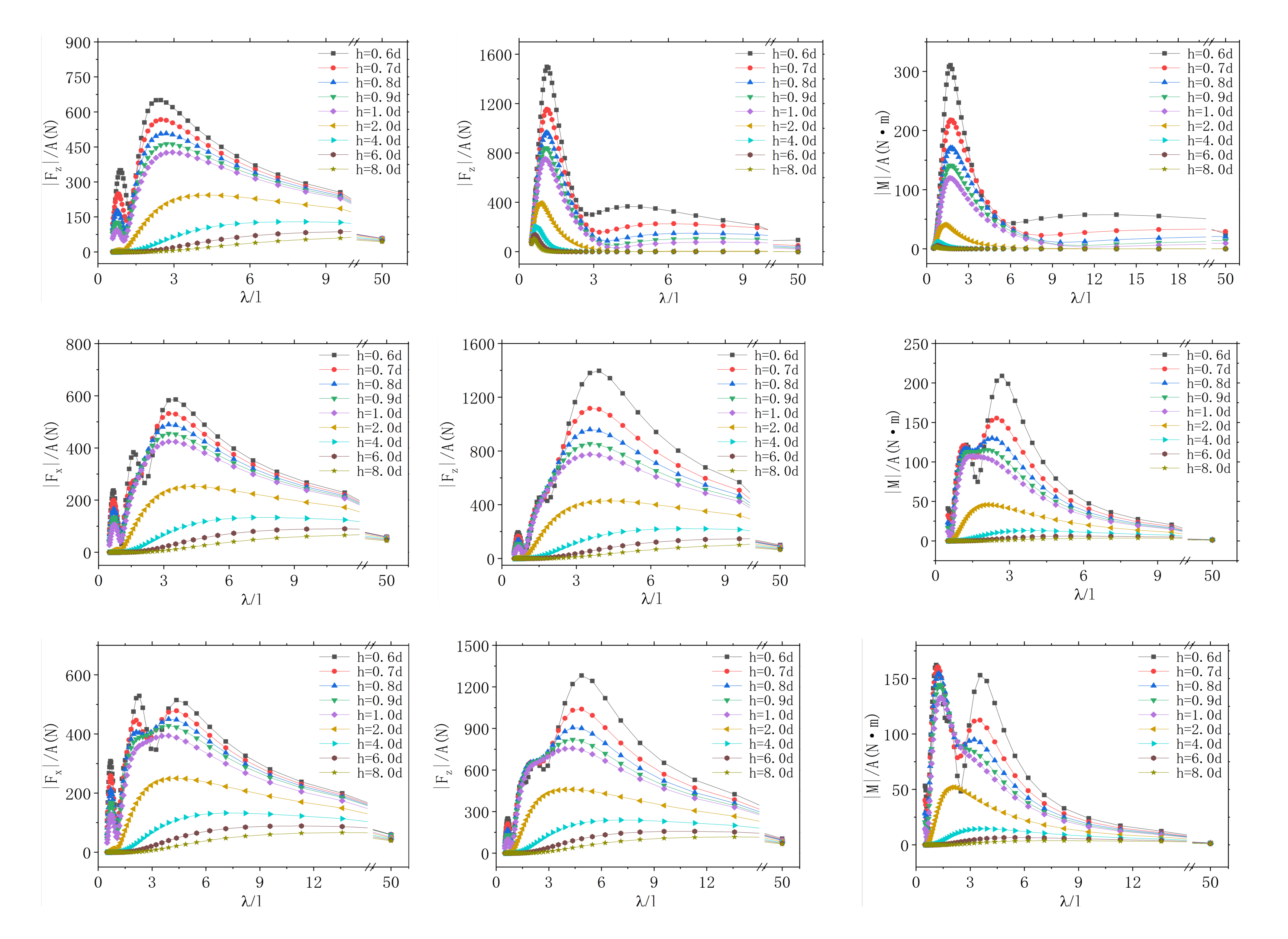
Figure 14.
Curves of wave force versus velocity of the Shark-AUV at different submerged depths. From the left column to the right column are the longitudinal force, vertical force and pitch moment of the AUV at the speeds of 0 m/s, 0.5 m/s and 1 m/s.
Figure 14.
Curves of wave force versus velocity of the Shark-AUV at different submerged depths. From the left column to the right column are the longitudinal force, vertical force and pitch moment of the AUV at the speeds of 0 m/s, 0.5 m/s and 1 m/s.
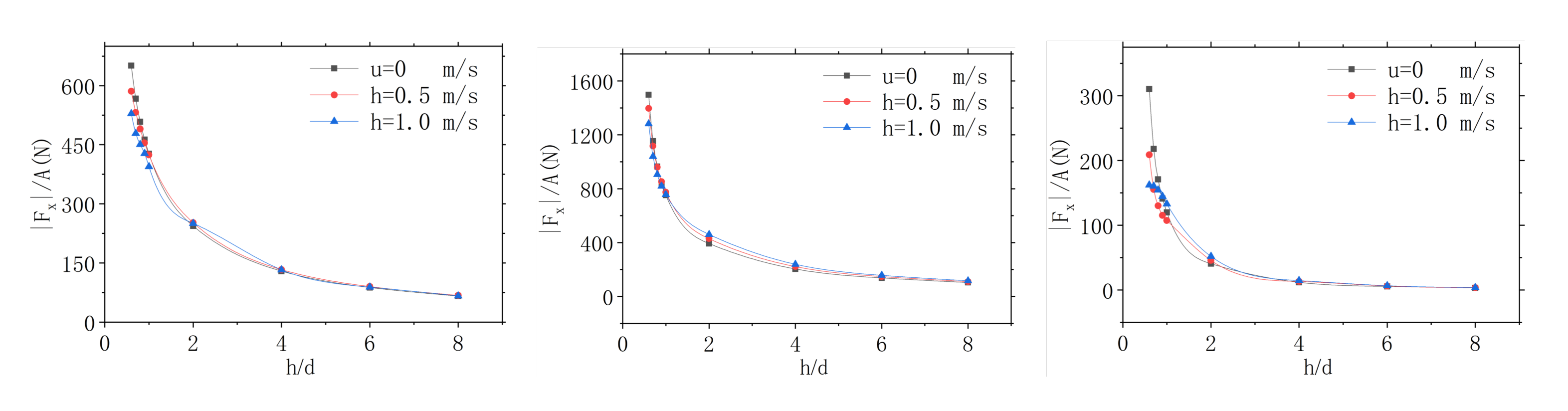
Figure 15.
From left to right: maximum longitudinal force, vertical force, and pitch moment at different submerged depths.
Figure 15.
From left to right: maximum longitudinal force, vertical force, and pitch moment at different submerged depths.
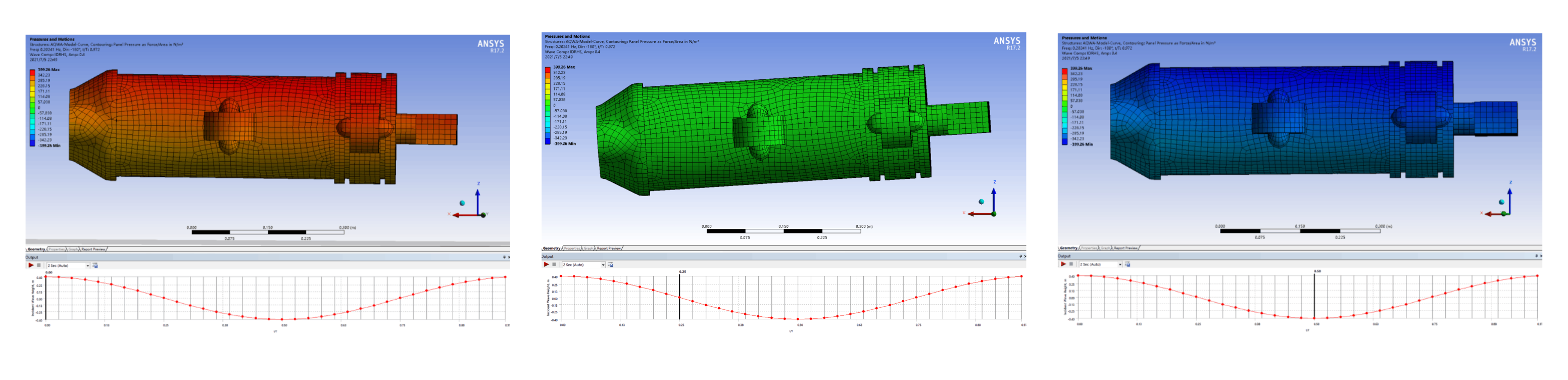
Figure 16.
Surface pressure nephogram of the Shark-AUV at different location of the wave, from left to right: crest, balance state, and trough.
Figure 16.
Surface pressure nephogram of the Shark-AUV at different location of the wave, from left to right: crest, balance state, and trough.
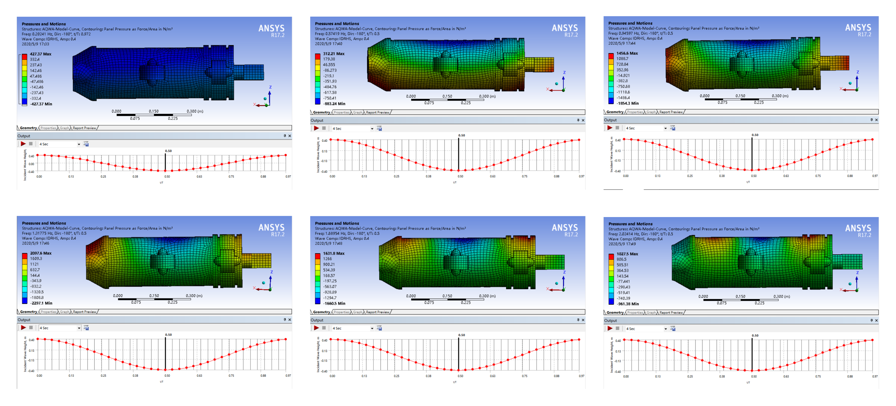
Figure 17.
From top to bottom, from left to right: surface pressure nephogram of the Shark-AUV at different wave frequencies (f = 0.20241 Hz, 0.57419 Hz, 0.94597 Hz, 1.31775 Hz, 1.58594 Hz, 2.02414 Hz) when the AUV moves in a head wave and is located in the trough with a wave amplitude of 0.4 m.
Figure 17.
From top to bottom, from left to right: surface pressure nephogram of the Shark-AUV at different wave frequencies (f = 0.20241 Hz, 0.57419 Hz, 0.94597 Hz, 1.31775 Hz, 1.58594 Hz, 2.02414 Hz) when the AUV moves in a head wave and is located in the trough with a wave amplitude of 0.4 m.
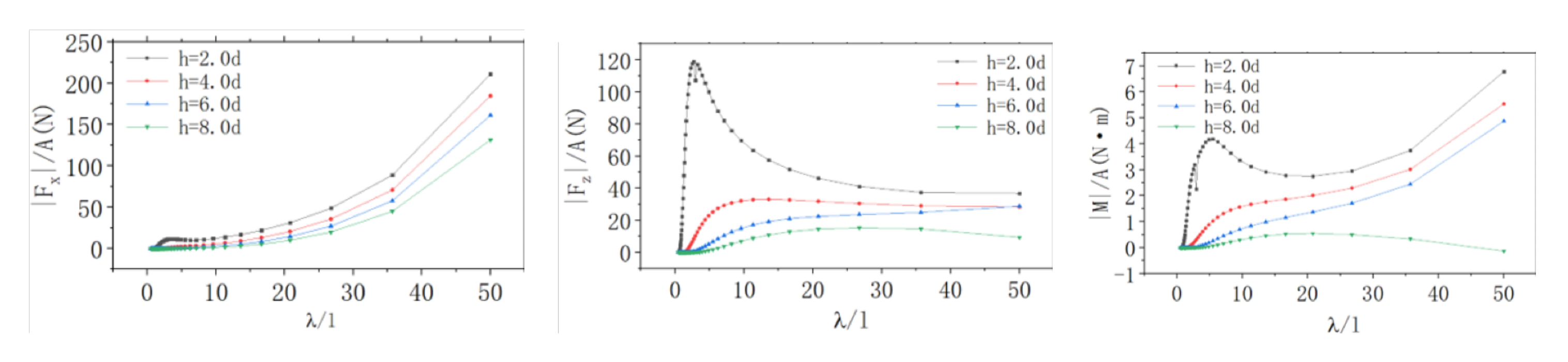
Figure 18.
From left to right: second-order wave forces of the Shark-AUV in longitudinal, vertical, and pitch directions at different submerged depths and different wavelengths.
Figure 18.
From left to right: second-order wave forces of the Shark-AUV in longitudinal, vertical, and pitch directions at different submerged depths and different wavelengths.
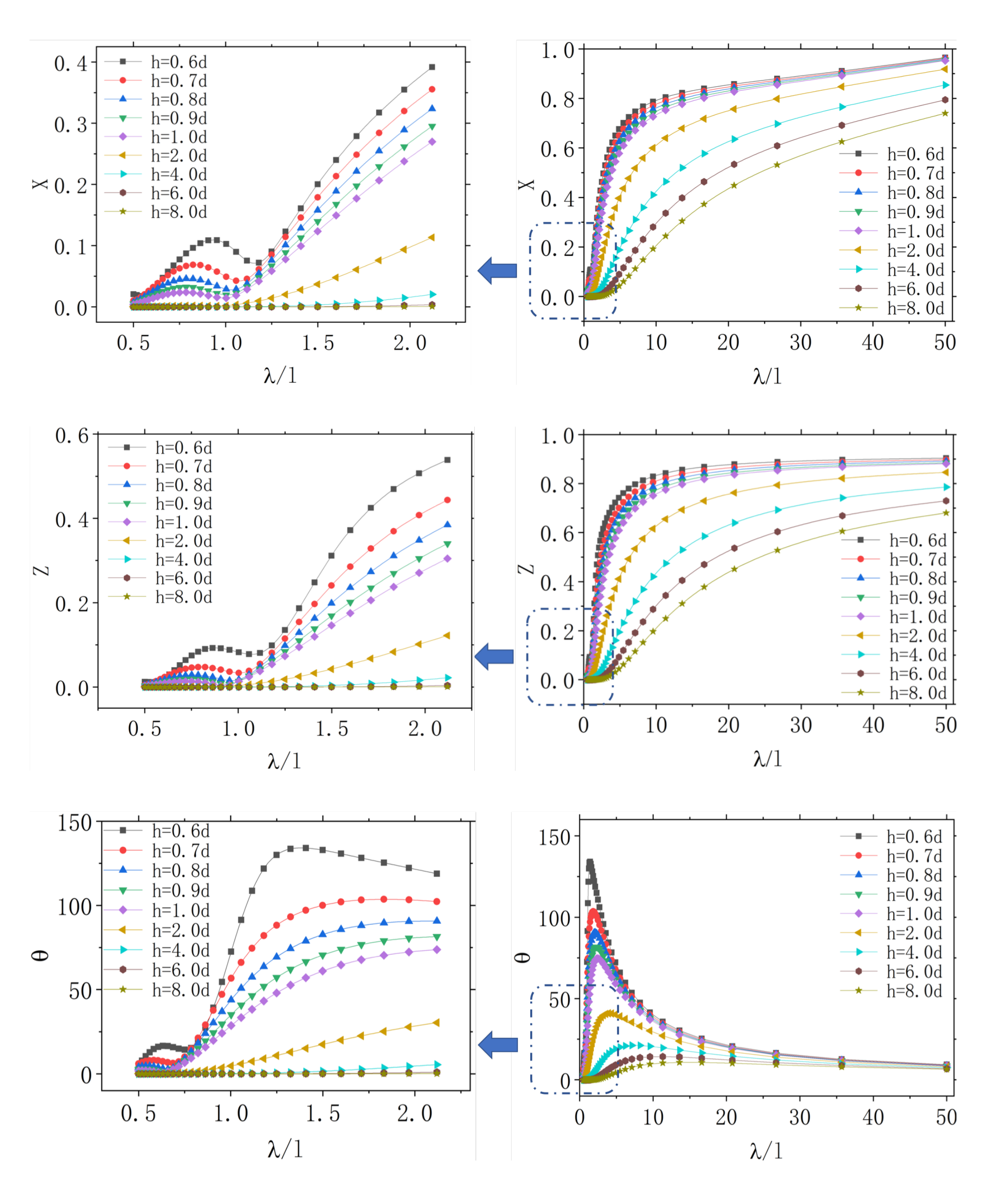
Figure 19.
From top to bottom: Curves of surge RAO, heave RAO, and pitch RAO versus wavelength.
Figure 19.
From top to bottom: Curves of surge RAO, heave RAO, and pitch RAO versus wavelength.
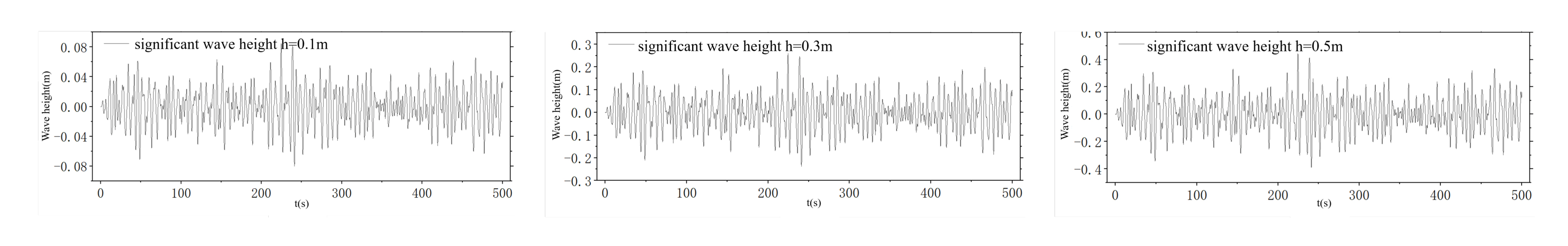
Figure 20.
From left to right: wave surface curve of PM dual-parameter spectrum under different significant wave heights (0.1 m, 0.3 m, 0.5 m).
Figure 20.
From left to right: wave surface curve of PM dual-parameter spectrum under different significant wave heights (0.1 m, 0.3 m, 0.5 m).
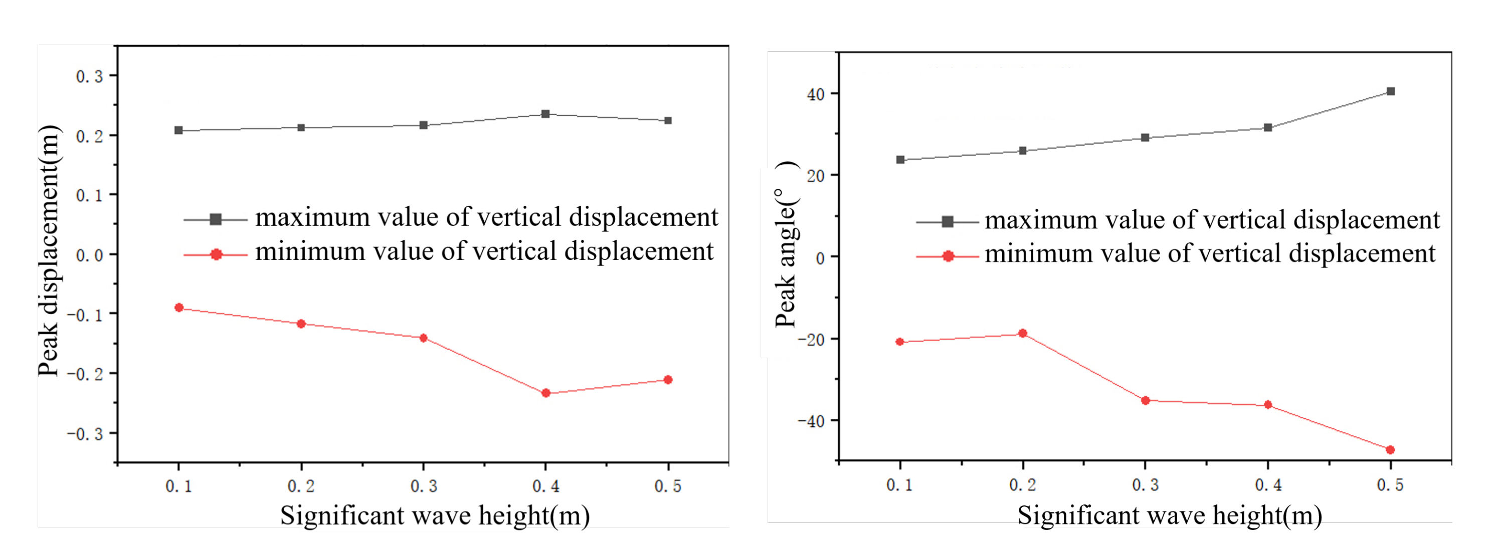
Figure 21.
Curves of the maximum vertical displacement and pitch angle of the Shark-AUV versus the significant wave height.
Figure 21.
Curves of the maximum vertical displacement and pitch angle of the Shark-AUV versus the significant wave height.
Figure 22.
SUBOFF model without appendage and its computational domain.
Figure 22.
SUBOFF model without appendage and its computational domain.
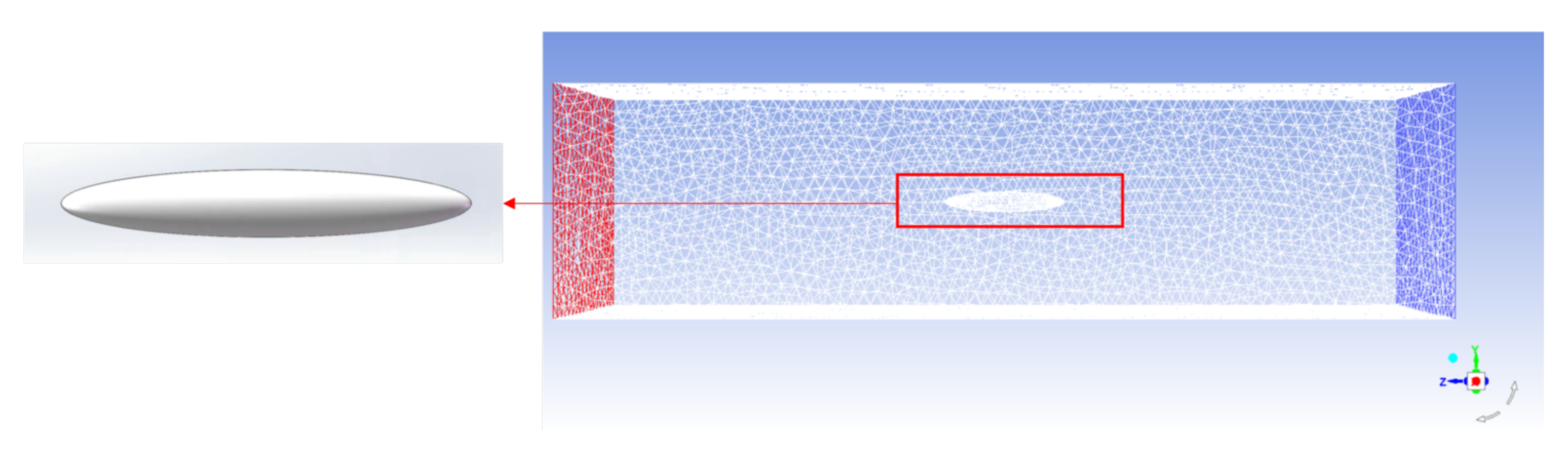
Figure 23.
Standard ellipsoid model and its computational domain.
Figure 23.
Standard ellipsoid model and its computational domain.
Figure 24.
3D model of the 21UUV.
Figure 24.
3D model of the 21UUV.
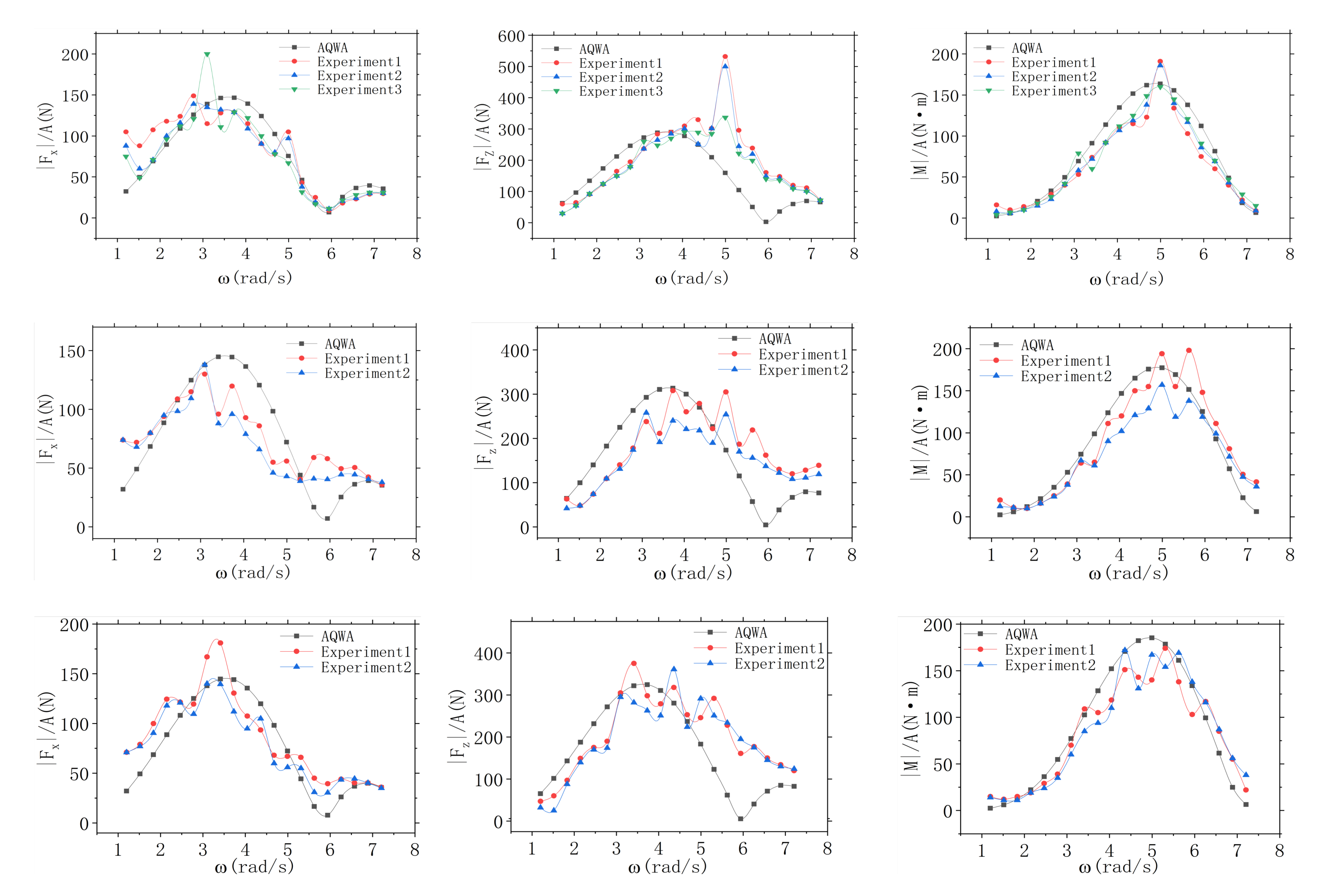
Figure 25.
Verification of numerical investigation results of wave force based on the 21UUV model. From the top row to the bottom row: curves of the longitudinal force, vertical force and pitching moment versus the wave circular frequency when u = 0 m/s, 0.489 m/s, 0.733 m/s.
Figure 25.
Verification of numerical investigation results of wave force based on the 21UUV model. From the top row to the bottom row: curves of the longitudinal force, vertical force and pitching moment versus the wave circular frequency when u = 0 m/s, 0.489 m/s, 0.733 m/s.
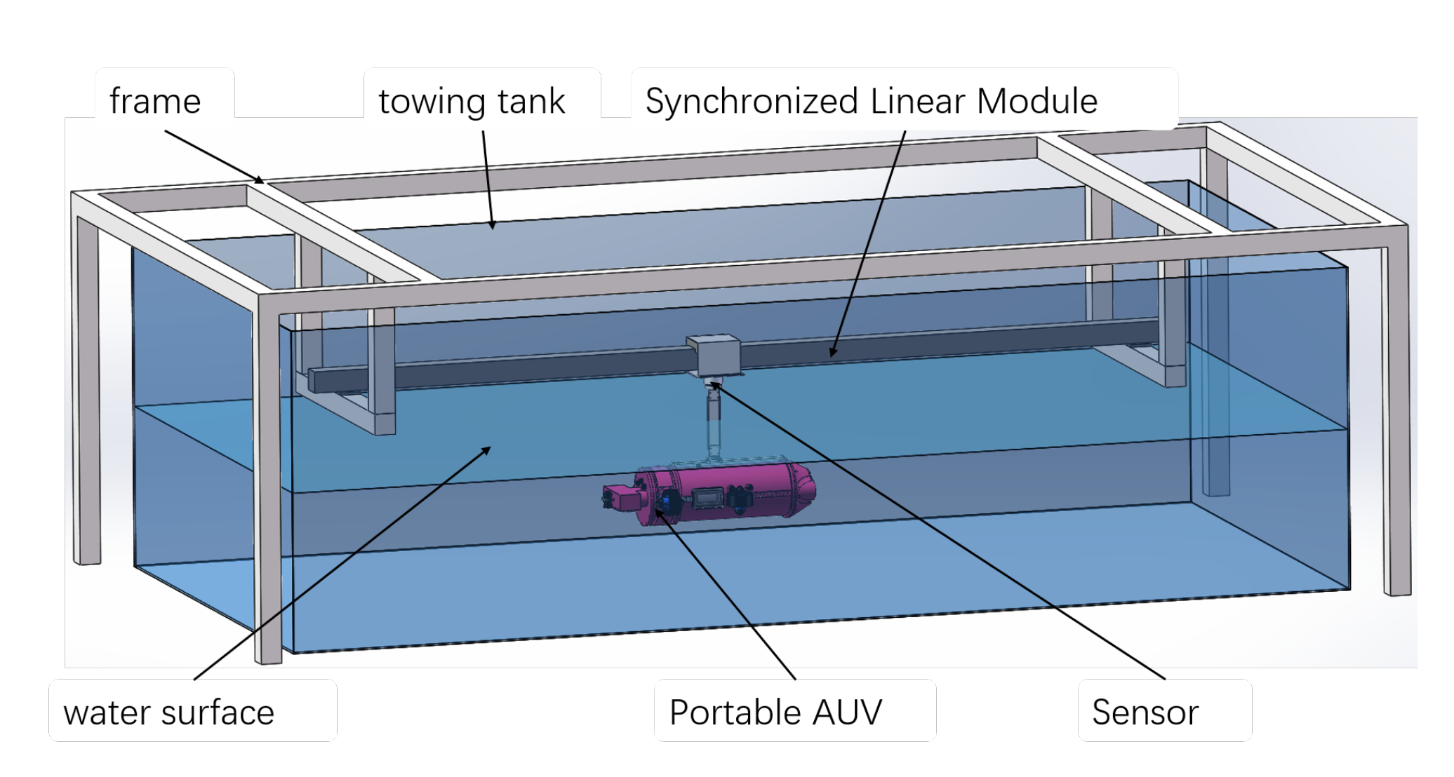
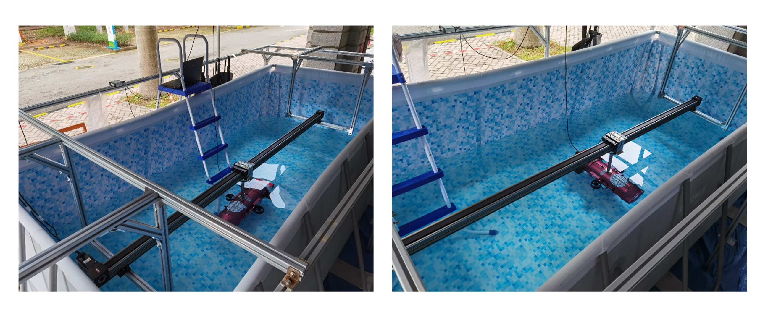
Figure 26.
Framework introduction of the designed physical experiment platform.
Figure 26.
Framework introduction of the designed physical experiment platform.
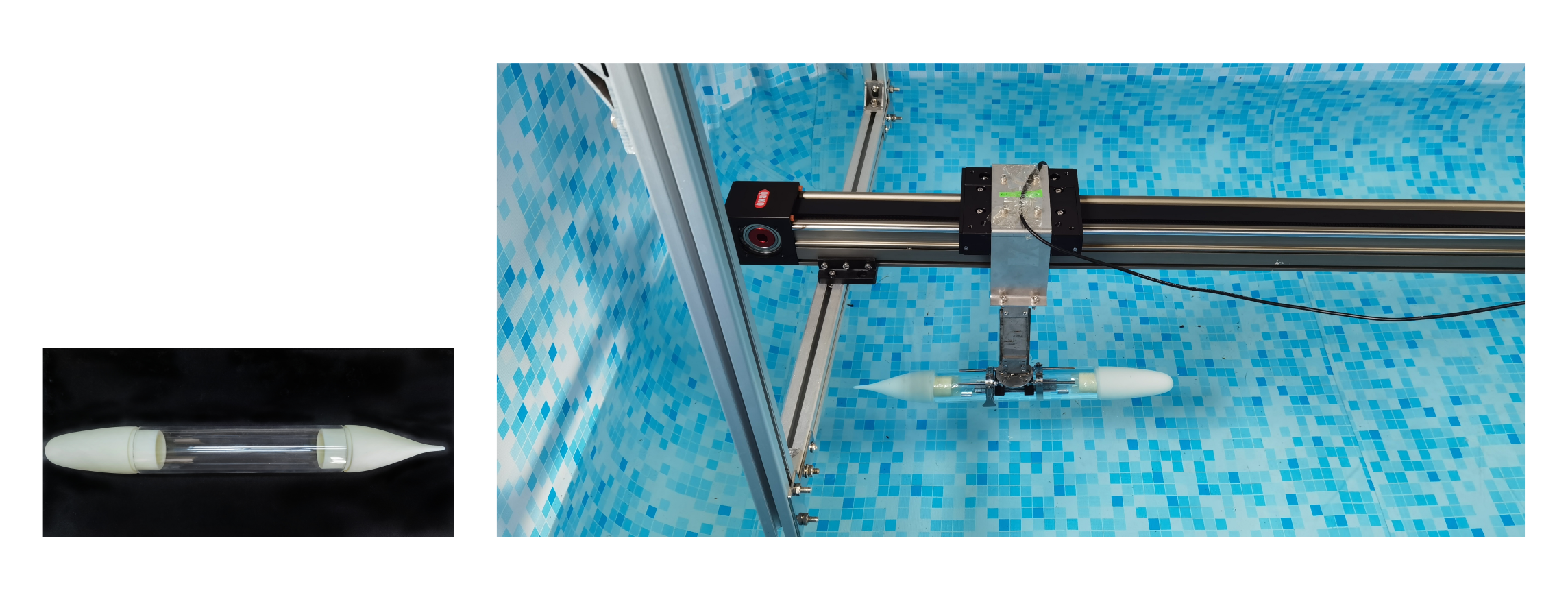
Figure 27.
SUBOFF model and its towing experiment setup in our physical experiment platform.
Figure 27.
SUBOFF model and its towing experiment setup in our physical experiment platform.
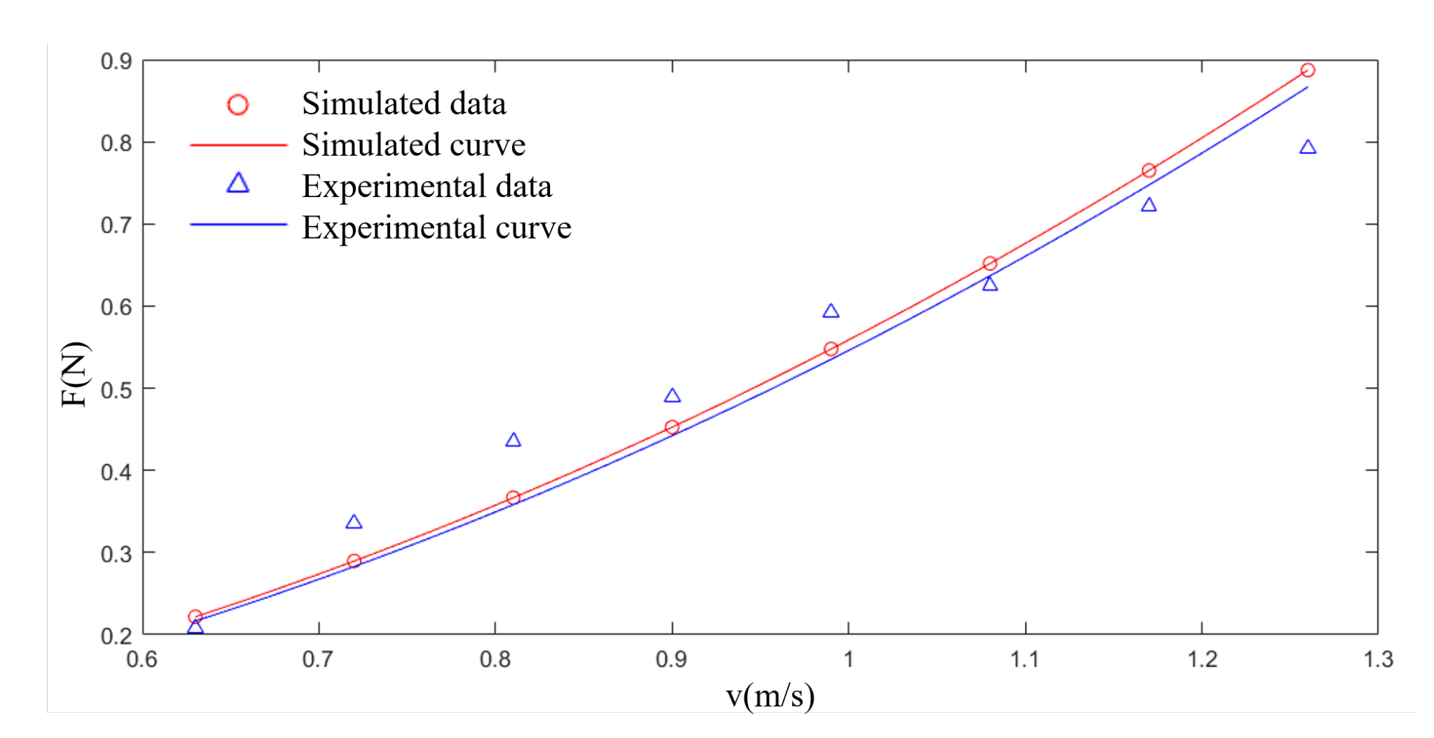
Figure 28.
Comparison of physical experimental results and CFD simulation results based on the SUBOFF model.
Figure 28.
Comparison of physical experimental results and CFD simulation results based on the SUBOFF model.
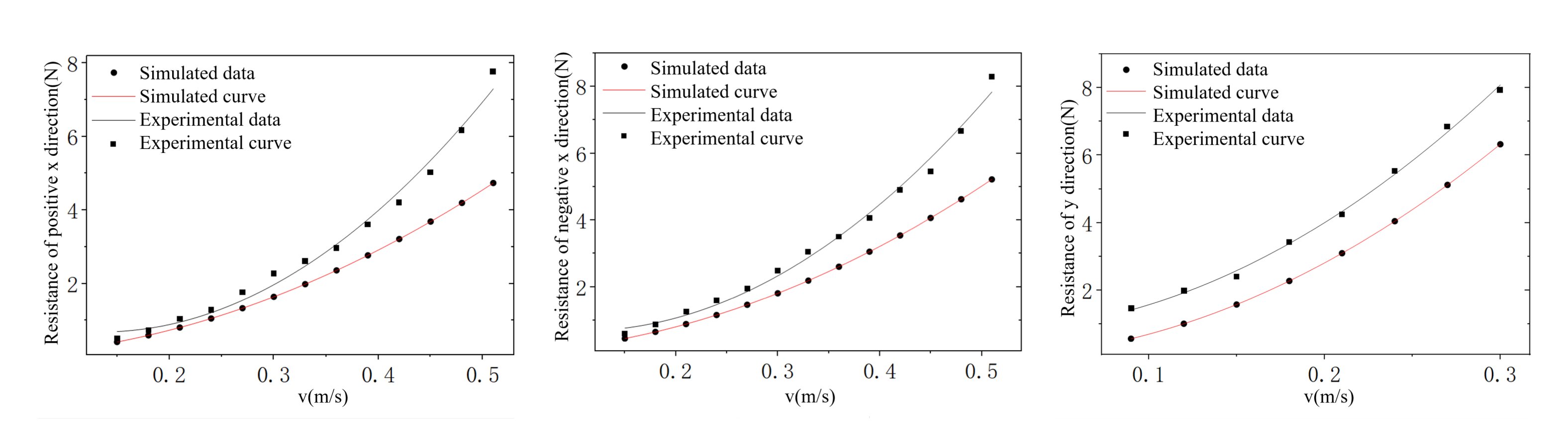
Figure 29.
Hydrodynamic coefficient estimation of the Shark-AUV based on the established physical experiment platform. The left diagram shows cruising forward along the x-direction, and the right one shows cruising forward along the y-direction.
Figure 29.
Hydrodynamic coefficient estimation of the Shark-AUV based on the established physical experiment platform. The left diagram shows cruising forward along the x-direction, and the right one shows cruising forward along the y-direction.
Figure 30.
Comparison of hydrodynamic coefficients obtained by CFD method and physical experiment platform. From left to right: the comparison results in -direction, the comparison results in -direction, and the comparison results in y-direction.
Figure 30.
Comparison of hydrodynamic coefficients obtained by CFD method and physical experiment platform. From left to right: the comparison results in -direction, the comparison results in -direction, and the comparison results in y-direction.
Table 1.
Setting of some initial parameters of CFD simulation.
Table 1.
Setting of some initial parameters of CFD simulation.
| Parameters | Initial Setting of the Parameters |
|---|
| Time | Steady (unsteady) motion is steady (transient) state |
| Turbulence model | RNG model |
| Discrete format | Second-order upwind discrete scheme |
| Solving algorithm | PISO |
| Fluid type | Liquid, density is 998.2 kg/, others are default |
| Time step | 1500 steps in steady motion and 100 steps per cycle |
| | in unsteady motion |
Table 2.
Numerical estimation of heave motion simulation of the Shark-AUV.
Table 2.
Numerical estimation of heave motion simulation of the Shark-AUV.
| | | | | | | |
|---|
| 0.2 | 1.256 | −0.19240 | 0.10053 | 0.0198 | −0.0050 | −0.0055 | 0.0030 |
| 0.4 | 2.513 | −0.76961 | 0.20106 | 0.0892 | −0.0202 | −0.0180 | 0.0088 |
| 0.6 | 3.769 | −1.73162 | 0.30159 | 0.2011 | −0.0664 | −0.0240 | 0.0197 |
| 0.8 | 5.026 | −3.07843 | 0.40212 | 0.3413 | −0.1011 | −0.0359 | 0.0376 |
| 1 | 6.283 | −4.81005 | 0.50265 | 0.5016 | −0.1558 | −0.0397 | 0.0392 |
Table 3.
Summary of the estimated hydrodynamic coefficients by towing experiment and PMM experiment simulation.
Table 3.
Summary of the estimated hydrodynamic coefficients by towing experiment and PMM experiment simulation.
| Coefficients | Value | Coefficients | Value | Coefficients | Value | Coefficients | Value | Coefficients | Value | Coefficients | Value |
|---|
| −0.0131 | | 0.5076 | | 0 | | 0.0007 | | 0.0009 | | 0.0003 |
| −0.3618 | | −0.6681 | | −0.2036 | | 0.0754 | | −0.1936 | | −0.0138 |
| −0.1043 | | −0.0948 | | 0 | | −0.0773 | | −0.0131 | | 0.0138 |
| 0.0147 | | −0.0007 | | 0 | | −0.0227 | | −0.1043 | | −0.0289 |
| −0.0007 | | −0.0754 | | 0.0044 | | 0 | | −0.1550 | | −0.0219 |
| 0.0131 | | −0.0017 | | −0.0056 | | −0.0754 | | −0.3805 | | 0.0852 |
| 0.1043 | | −0.3467 | | 0.0852 | | −0.0852 | | −0.0172 | | −0.0718 |
| 0.0003 | | 0.0351 | | −0.1126 | | 0.0047 | | 0 | | 0.0216 |
| 0 | | 0.0043 | | −0.0179 | | −0.0131 | | −0.3389 | | 0.0001 |
| 0.0391 | | 0.0097 | | | | | | | | |
Table 4.
Comparison the result of our method with that of the NSWCCD [
38].
Table 4.
Comparison the result of our method with that of the NSWCCD [
38].
| Speed (kont) | 5.92 | 10.00 | 11.84 | 13.92 | 16.00 | 17.99 |
|---|
| NSWCCD results (N) | 87.4 | 242.2 | 332.9 | 451.5 | 576.9 | 697.0 |
| RNG k- results (N) | 92.59 | 244.86 | 335.84 | 454.76 | 590.63 | 736.10 |
| Error(%) | 5.94 | 1.10 | 0.88 | 0.72 | 2.38 | 5.61 |
| SST k- results (N) | 89.73 | 237.71 | 325.85 | 441 | 573.38 | 713.01 |
| Error(%) | 2.67 | 1.85 | 2.12 | 2.33 | 0.78 | 2.3 |
Table 5.
Comparison of results of our method with the experiment in [
39].
Table 5.
Comparison of results of our method with the experiment in [
39].
| Hydrodynamic Coefficient | | | | |
|---|
| Numerical solution | −0.0266 | −0.0230 | −8.466 × 10⁻⁵ | 0.0232 |
| Standard solution | −0.0268 | −0.0186 | 0 | 0.0186 |
| Error (%) | 0.7 | 23.7 | 0 | 24.7 |
Table 6.
Parameters of the 21UUV and the reported experiment.
Table 6.
Parameters of the 21UUV and the reported experiment.
| Parameters | Parameters Setting |
|---|
| Size | L = 1.786 m, D = 0.27 m |
| Distance to the sea surface | 0.379 m |
| sailing speed in the surface waves | = 0 m/s, = 0.489 m/s, = 0.733 m/s |
| Amplitude of the waves | = 0.014 m, = 0.028 m, = 0.037 m |
| Circle frequency range of the waves | w = 1.200 to 7.207 rad/s |


