2.1. Mathematical and Numerical Model
To perform the numerical simulations in this study, ANSYS Fluent software was used, which is a computational fluid dynamics (CFD) commercial code based on the finite volume method (FVM). This software provides comprehensive modeling capabilities for a wide range of incompressible and compressible, laminar and turbulent fluid flow problems [
41].
In this study, to tackle with water–air interaction, a nonlinear multiphase model was employed. The motion of fluid flow throughout the mixture is described by the continuity equation and the momentum conservation equations, which, for a two-dimensional domain, are as follows [
42,
43]:
where
u and
w are the velocity components in
x and
z directions (m/s), respectively,
is density (kg/m
),
t is time (s),
p is static pressure (N/m
),
is the absolute viscosity coefficient (kg/m·s),
S is a damping sink term used in the numerical beach, and
is the gravitational body force (N/m
).
It is worth mentioning that Reynolds averaged Navier–Stokes (RANS) equations were used, which are based on the decomposition of the instantaneous velocity and pressure fields of the Navier–Stokes equations into mean and fluctuating components, and the subsequent time-averaging of the set of equations. This process introduces Reynolds stress terms associated with turbulence [
44]. Thus, in addition to analyzing the domain in a laminar flow regime, two turbulence models which could close the set of equations were compared:
k-
and shear stress transport (SST)
k-
turbulence models.
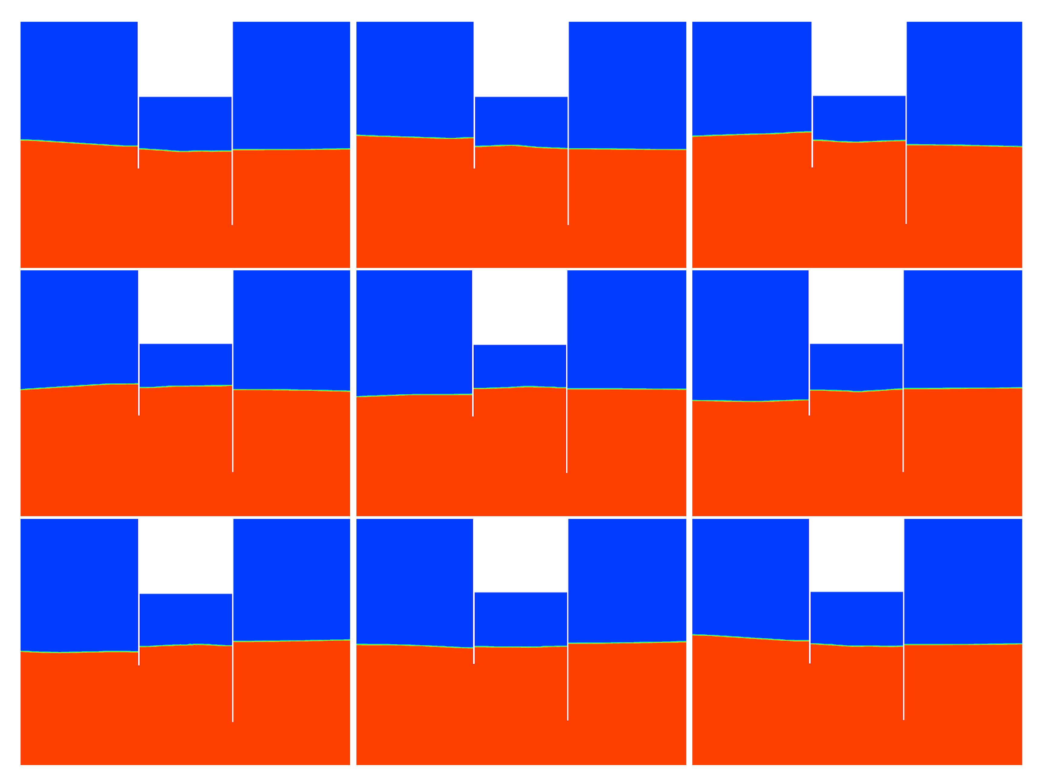
The nonlinear multiphase model adopted uses the surface-tracking volume of fluid (VOF) technique [
45], which can model two or more immiscible fluids and track the volume fraction (
) of these fluids inside each element throughout the domain. Thus, according to volume fraction values for a domain composed of water and air, three situations are possible: if
is equal to 0, that means the cell is empty of water and filled exclusively by air; if
is equal to 1, that means the cell is full of water; and if
is equal to any other value between 0 and 1, that means the cell contains the interface between the two phases. The volume fraction for the two phases throughout the two-dimensional domain follows a transport equation as shown [
46,
47]:
The values for density and absolute viscosity coefficient, fluid properties present in the momentum conservation equations (Equations (
2) and (
3)) are then determined as follows [
47]:
As wave reflection may interfere with surface elevation along the channel, a numerical beach was inserted at the end of the domain. In this case, a damping sink term (
S) is added to the momentum equation for the cell zone in the vicinity of the pressure outlet boundary [
41]:
where
and
are linear and quadratic damping coefficients, respectively,
V is the velocity along vertical direction (m/s),
z is the distance from free surface level (m),
and
are the free surface and bottom coordinates along vertical direction (m), respectively,
x is the horizontal coordinate (m), and
and
are the start and end points of the numerical beach in the horizontal direction (m), respectively.
As previously mentioned, the methodology used in this study consists of generating numerical waves through the imposition of discrete transient data of orbital wave velocity in vertical and horizontal directions. To obtain the values used in the imposition of prescribed velocity boundary conditions, and to perform an analytical comparison with the results, the 2nd order Stokes wave equation was employed. Therefore, the horizontal and vertical wave velocity components and the water surface displacement (
) are [
11]:
where
H represents the wave height (m),
k is the wave number (m
),
h is the channel water depth (m), and
is the wave angular frequency (rad/s).
Lastly, to assist in comparing the results, the Normalized Root Mean Squared Error (NRMSE) for each simulation was measured. The NRMSE is calculated using the following equation [
48,
49]:
where
represents the values obtained from simulations,
represents the observation, i.e., the analytical solution or experimental results,
n is the number of observations available for analysis, and
and
indicate the maximum and minimum observation values, respectively.
2.2. Numerical Simulations
When dealing with numerical simulations of coastal scenarios, proper wave generation is a fundamental step to achieve reliable results. The computational domain in this case is a two-dimensional numerical wave channel (NWC), with a length of 65 m, which corresponds to approximately 9 times the wavelength (
L = 7.54 m), height of 6 m, and water depth (
h) of 4 m. As adopted by Lisboa et al. [
34], two wavelengths on the extremity of the NWC have been dedicated to be a numerical beach, thus being responsible for wave damping and avoiding wave reflection.
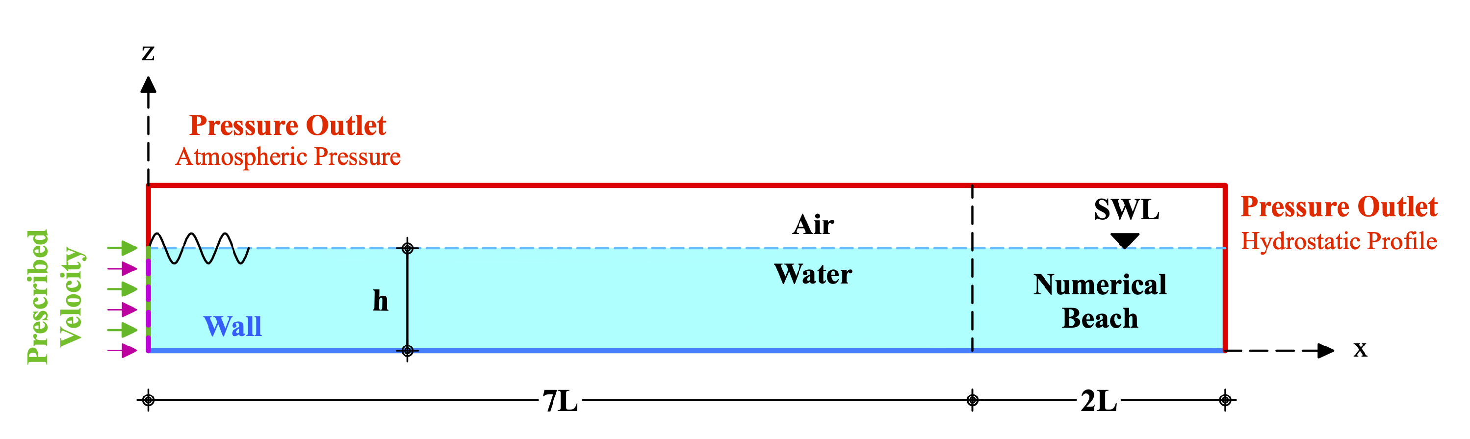
As mentioned, a NWC was simulated using the Fluent software applying the proposed methodology and two simulations were performed. The first simulation aimed to perform a verification of the wave generation and propagation, simulating 2nd order Stokes waves and then comparing the results with its analytical solution (Equation (
10)). For that, the following boundary conditions have been assigned to the computational domain, as shown in
Figure 2: on the left, in green and purple, the prescribed velocity boundary condition was assigned; at the bottom, in blue, the no-slip wall boundary condition was imposed; on the left and at the top, in red, the pressure outlet boundary condition was used with an atmospheric pressure value of 101,325 Pa; lastly, on the right, a special pressure outlet boundary condition was assigned, using a hydrostatic pressure profile, as adopted by Lisboa et al. [
34]. Additionally, the surface water line (SWL) is represented by the dashed line.
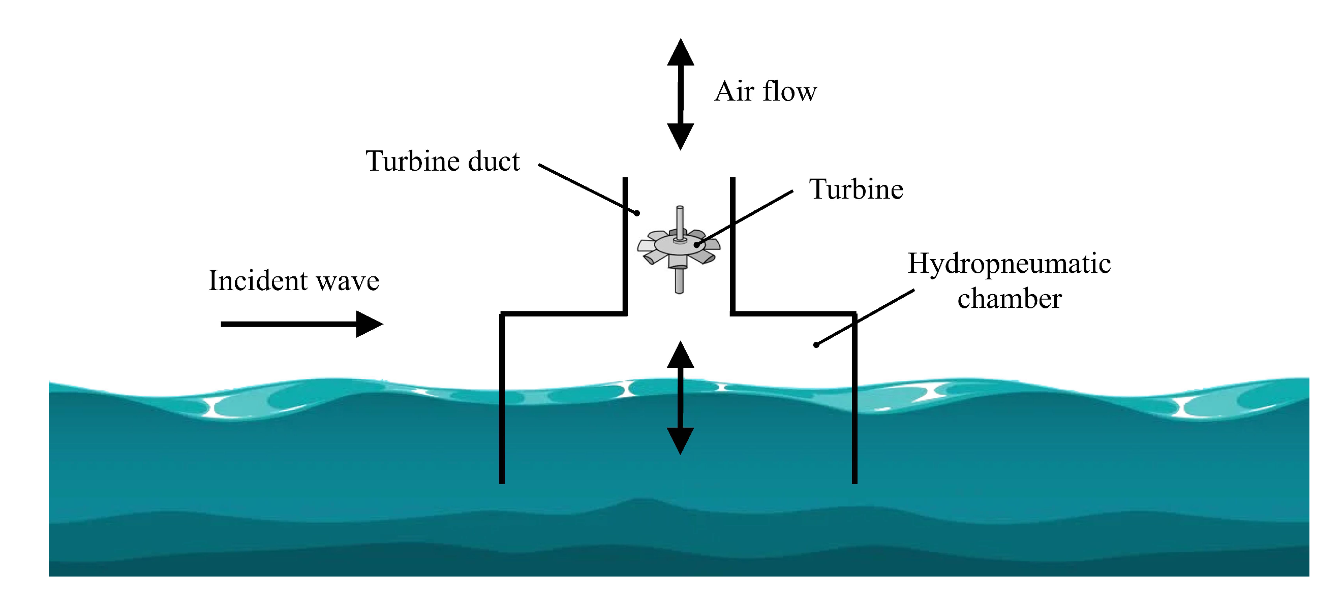
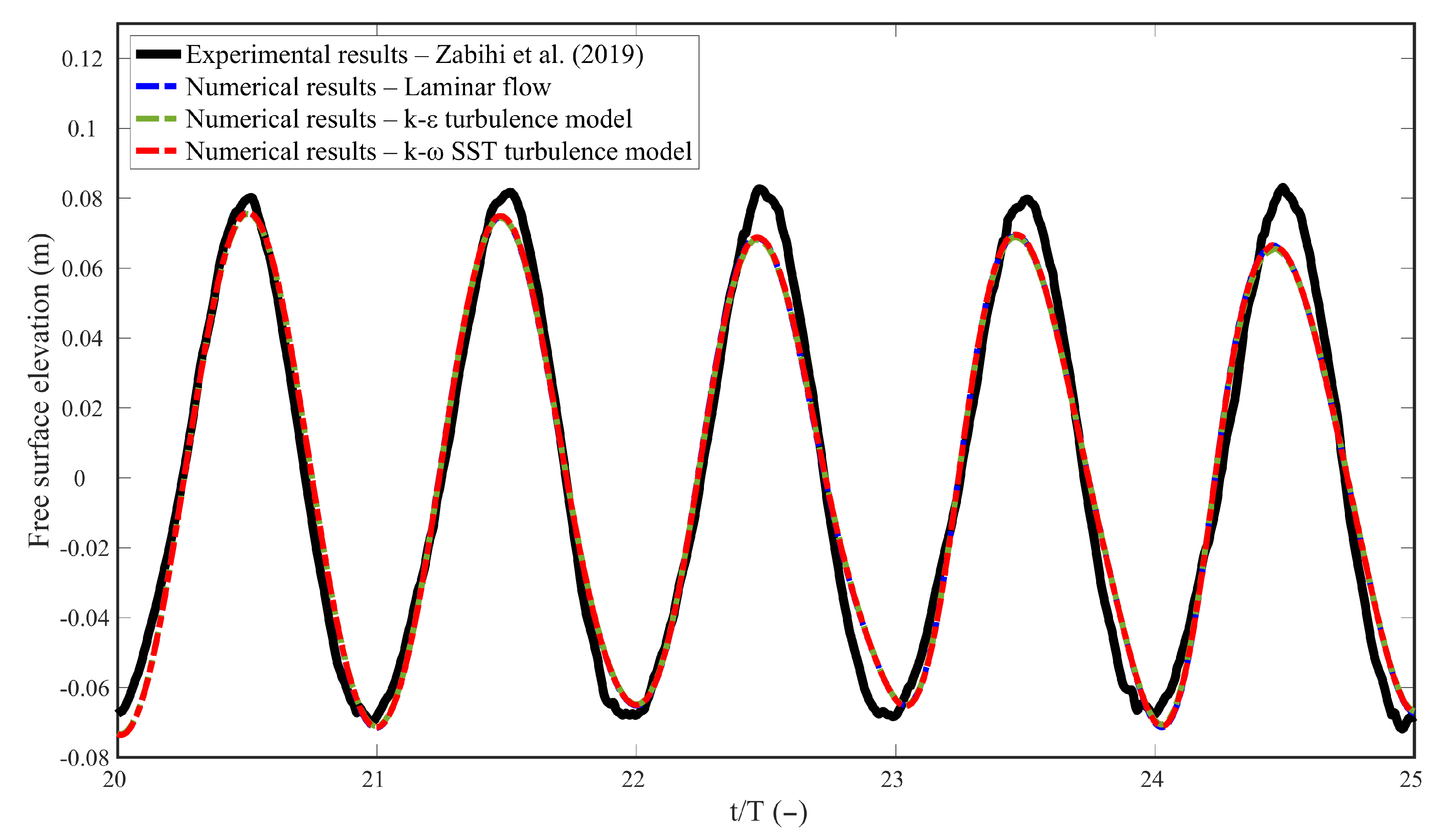
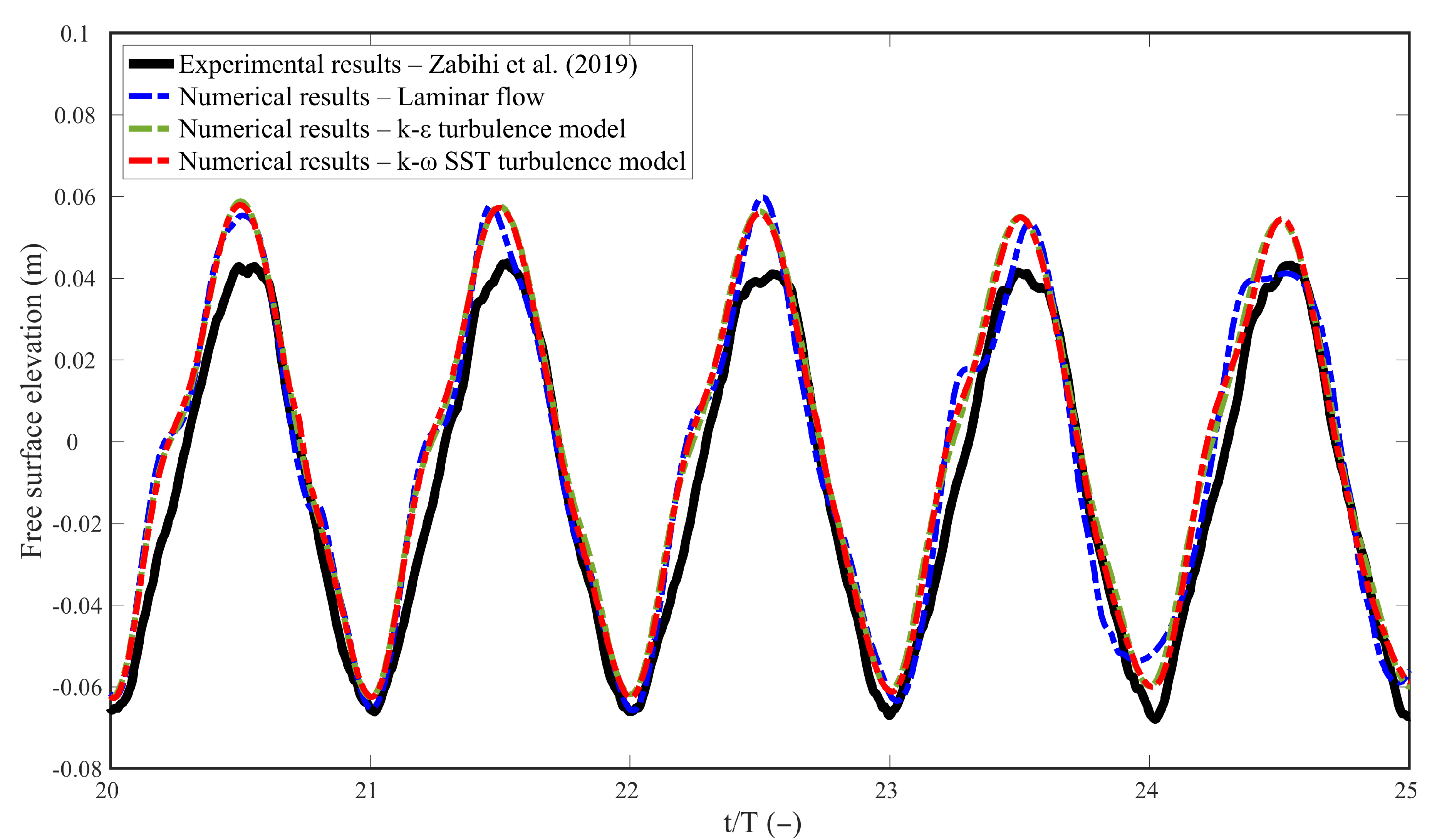
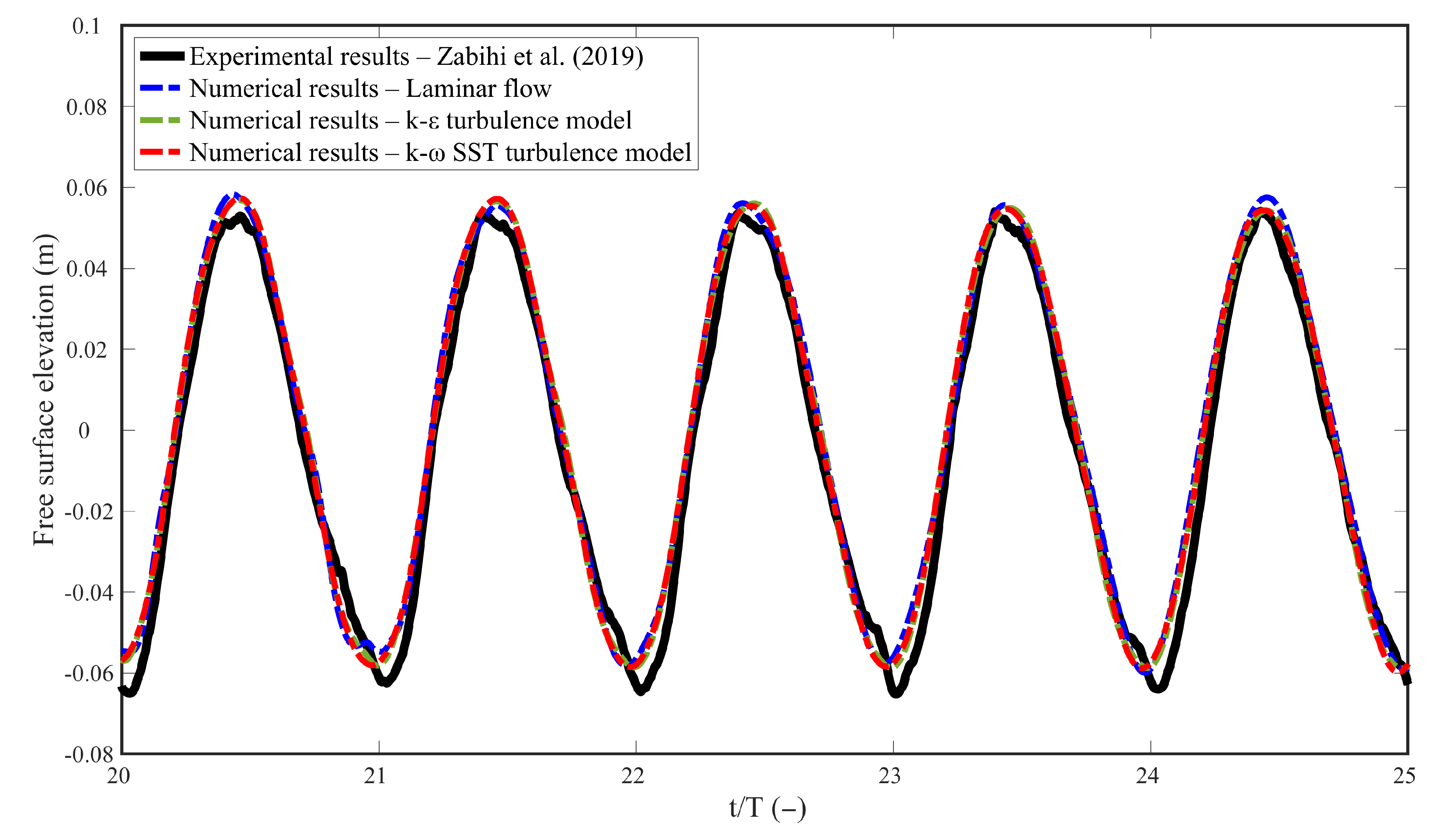
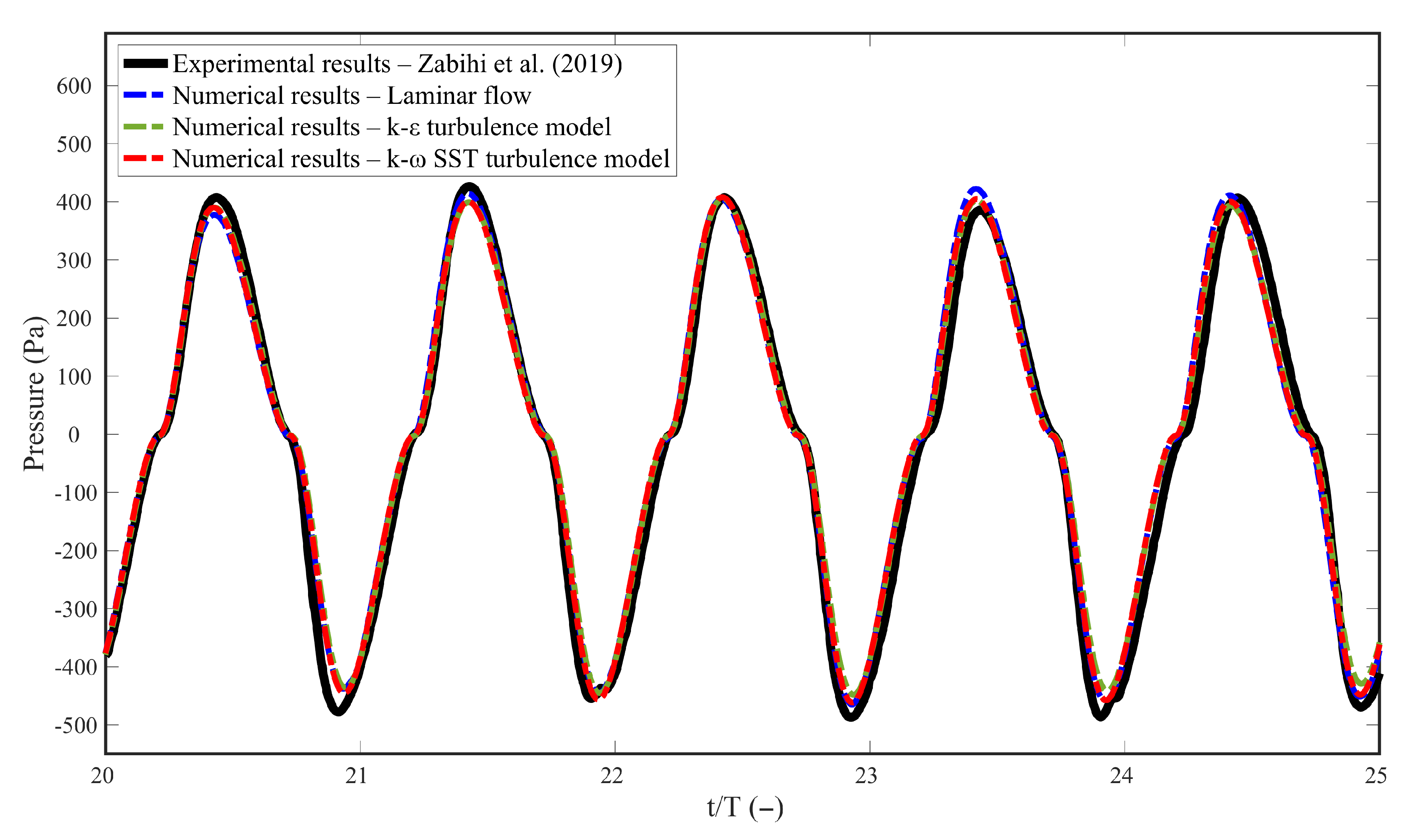
In the second simulation, the methodology was validated; an OWC device was inserted to reproduce a laboratory experiment performed by Zabihi et al. [
40]. The wave parameters adopted were the same for both simulations, where the height of the simulated wave was 0.15 m and its period was 2.2 s, following the values used in the experiment.
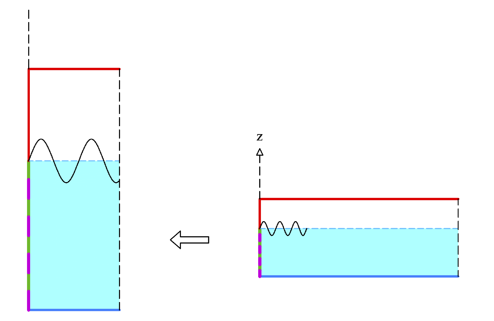
The proposed methodology was used to impose the prescribed velocity boundary condition. It presents a geometric particularity, which is, for discrete transient data imposition as boundary conditions of velocity inlet, it is necessary that this region of geometry is divided into subregions (green and purple lines), as shown in
Figure 3 [
9].
As shown in
Figure 2 and
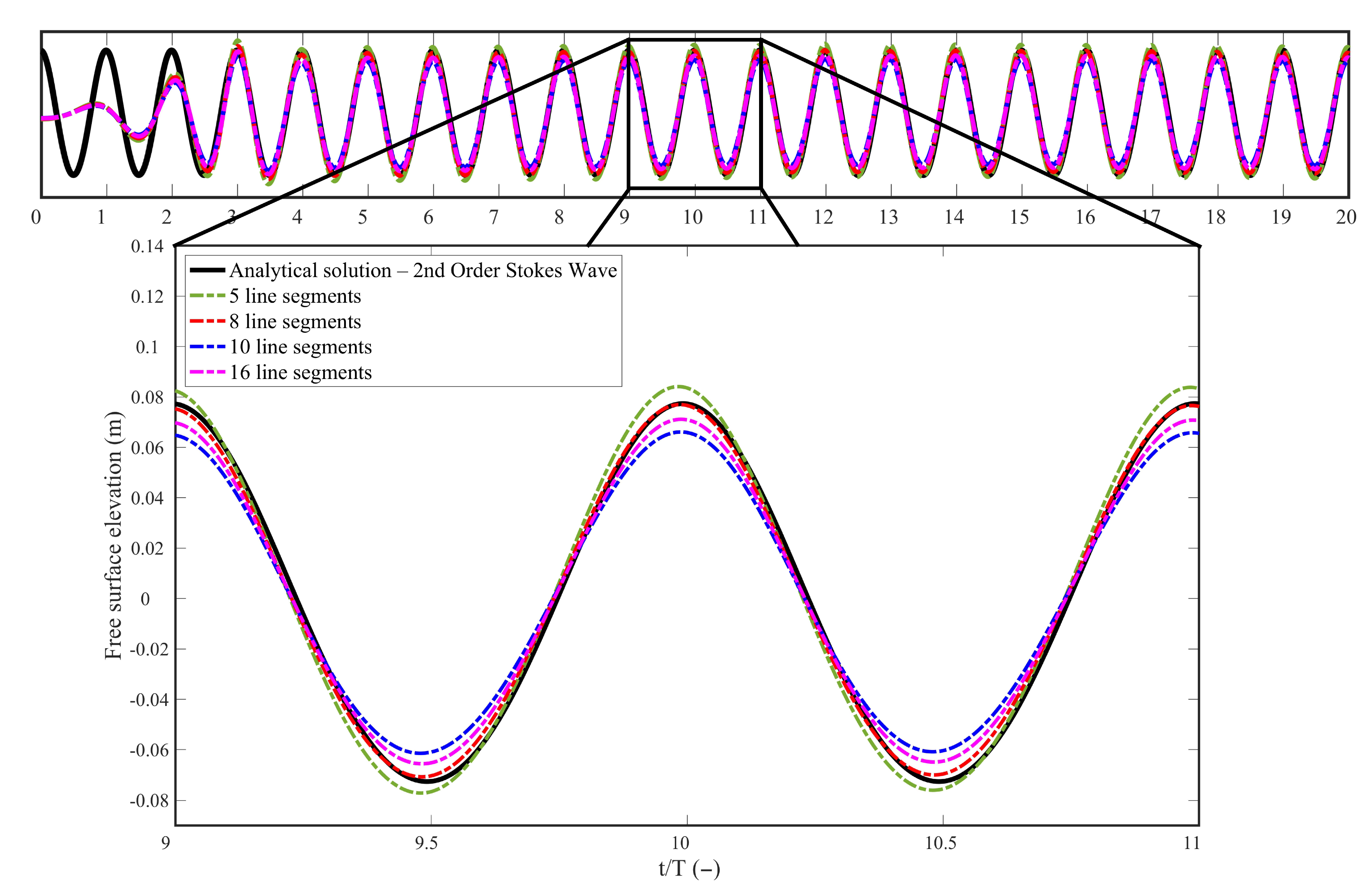
Figure 3, the prescribed velocity boundary condition is assigned to the line segments at the entrance of the channel. Each segment receives different values corresponding to the horizontal and vertical wave velocity components
u and
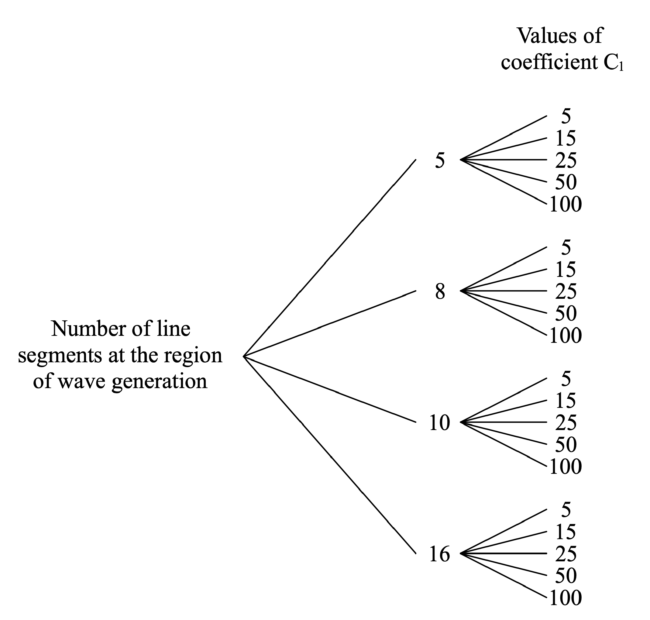
w, respectively. However, the optimal discretization, i.e., the number of line segments that provides a proper wave generation, must be analyzed. Therefore, the number of segments were evaluated over 2 min of simulation, comparing free surface elevation when using 5, 8, 10, and 16 line segments at the velocity inlet region.
Since the mean water level in the wave channel is 4 m, the length of each segment changes according to the total amount of segments. For example, when using 5 line segments at the entrance, each segment has a length of 0.80 m; when using 8 segments at the entrance, each one has a length of 0.50 m, and so on. The domain geometry and mesh were generated using GMSH software [
50].
As presented in
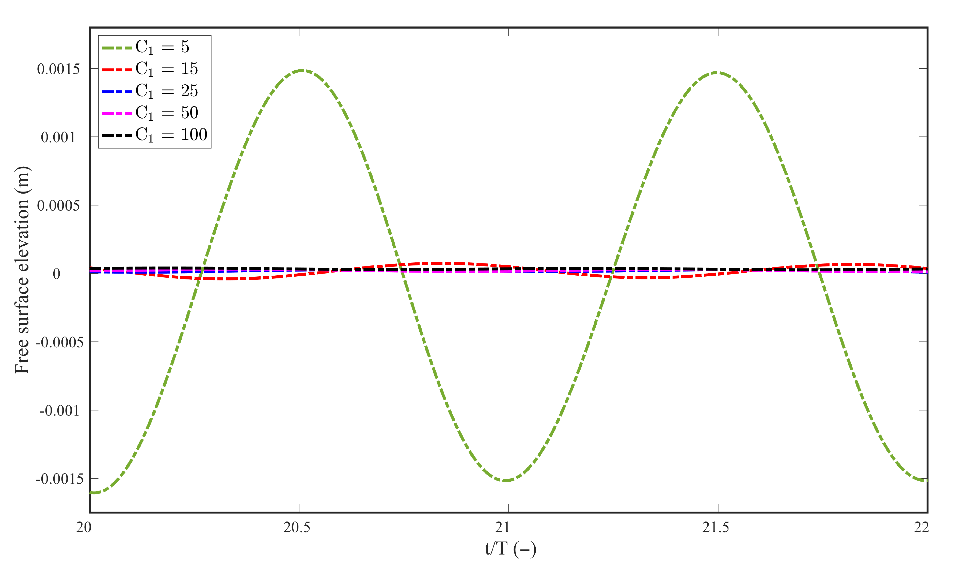
Section 2.1, the numerical beach equation has a linear (
) and a quadratic (
) damping coefficient, which allows for the calibration of the numerical beach. Similar calibrations were previously carried out, where good results were achieved with
= 0 [
34,
51]. Therefore, simultaneously to the velocity inlet boundary condition testing, 5 values of
were tested, as shown in
Figure 4, over simulations of 2 min to analyze the efficiency of these parameters.
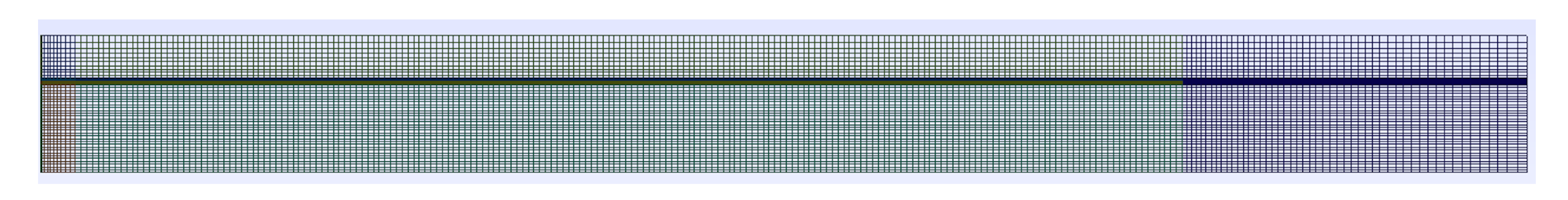
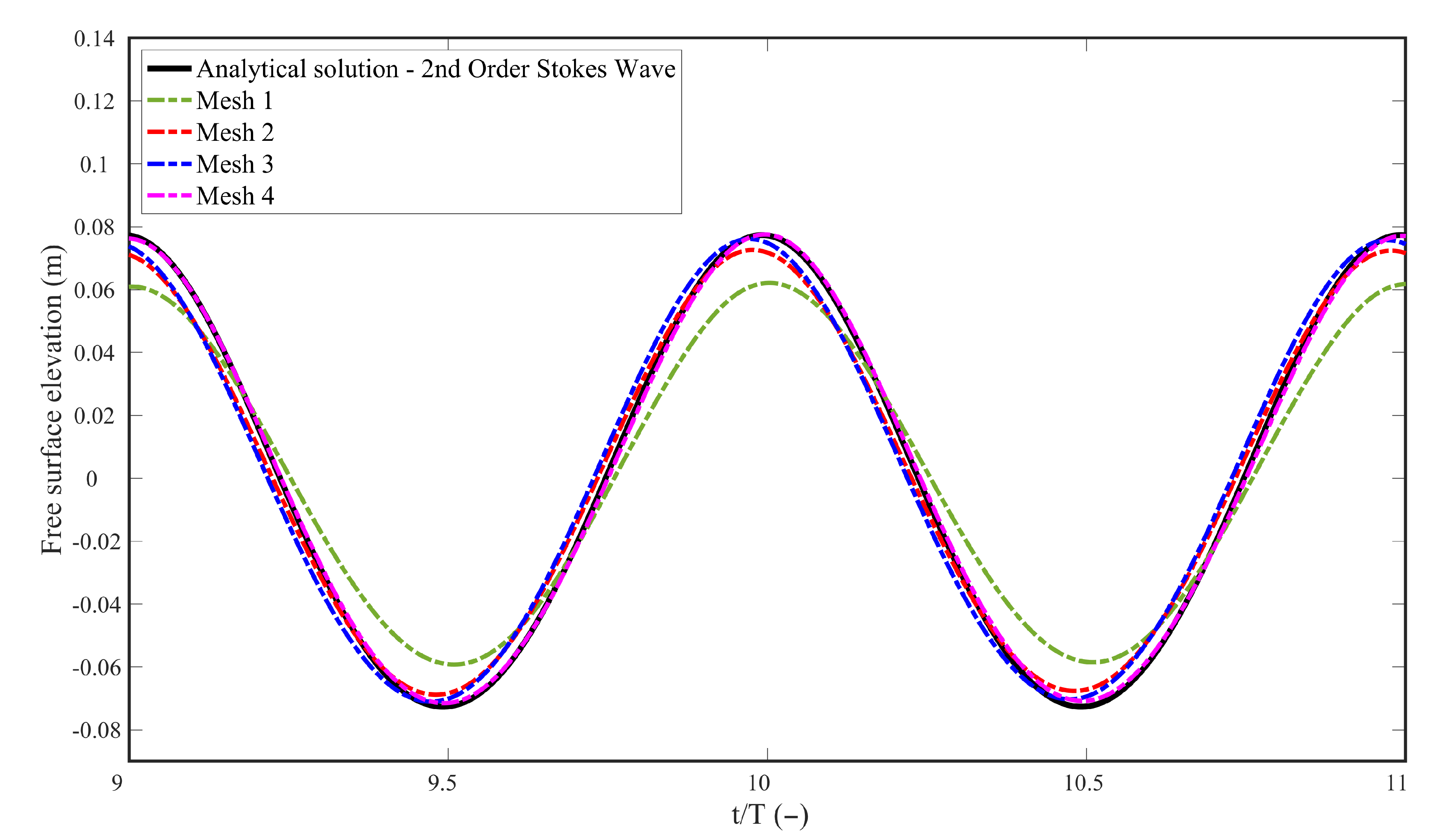
Once the numerical beach was calibrated, mesh discretization was studied. For that, four different mesh sets were analyzed. In each set, different horizontal and vertical sizes of mesh elements were tested, assuming the values shown in
Table 1, where
L is the wavelength and
H is the wave height. In addition, a refinement zone, with a height twice the height of the incoming wave, was applied to the area nearing the free surface, through the entire length of the channel. Outside the refinement zone, along the channel, elements had a square shape with equal length and height, as it can be seen in
Figure 5.
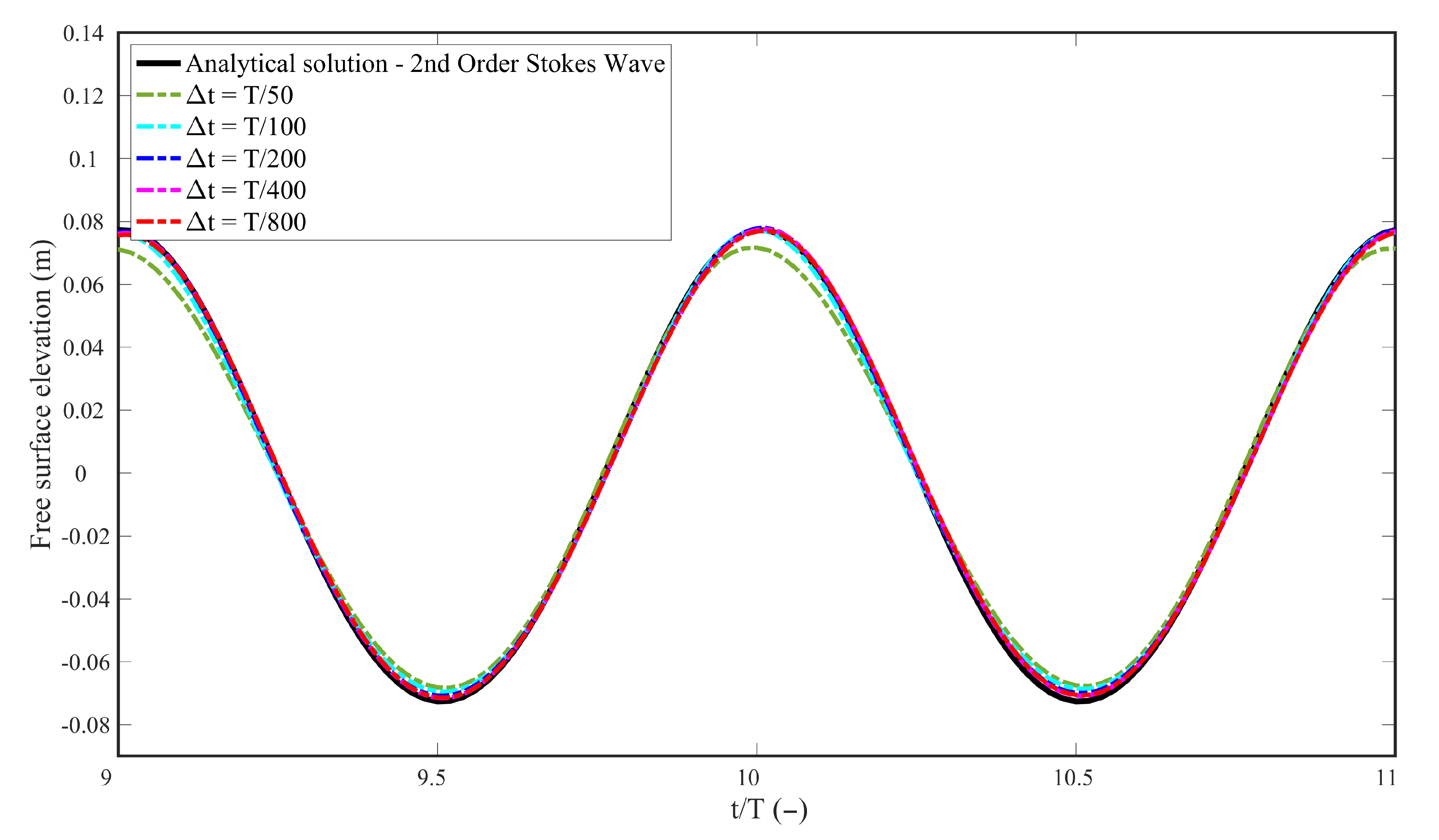
To ensure a proper wave generation, temporal discretization was also studied and time step (
) tests were performed. Liu et al. [
14] indicate that numerical accuracy is ensured when
is less than
T/50, where
T is the wave period. Therefore,
values of
T/50,
T/100,
T/200,
T/400, and
T/800 were tested. It is worth highlighting that, before this test was performed, the time step adopted for the simulations was T/400 [
40].
With all parameters tested, regular 2nd order Stokes waves were simulated in the channel and its results were compared with the analytical solution, given by Equation (
10). After all tests which ensure a proper wave generation, an OWC WEC device with the dimensions as those used by Zabihi et al. [
40] was inserted in the channel.
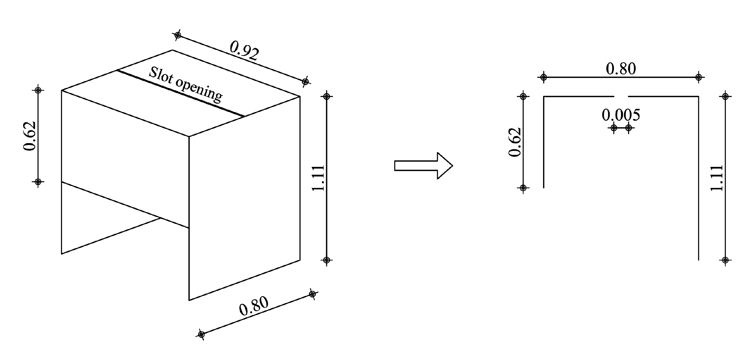
In the mentioned experiment, a fixed OWC model of 1:15 scale was used, with a length of 0.80 m, width of 0.92 m, and 1.11 m of height (
Figure 6). The experiments were performed in a wave tank 400 m long, 6 m wide, and 4 m high. Regular waves with a wave height of 0.15 m and three wave periods of 1.8, 2.0, and 2.2 s were used. It is worth mentioning the authors observed that short period waves entering the device could reflect from the chamber rear wall, interacting with incoming waves and resulting in higher nonlinearity; therefore, the 2.2 s wave period was adopted for the numerical simulations.
In addition, for the computational domain, a simplification regarding the experiments was made. In the laboratory, the distance between the OWC model and each side wall of the tank was 2.54 m; since this value is more than twice the width of the OWC model, wave reflection was considered negligible. Therefore, a two-dimensional computational domain was adopted for this study.
Figure 6 shows the dimensions of the physical model, as well as its cross-section, used in the two-dimensional computational domain, and
Figure 7 shows the computational domain used in the validation procedure.
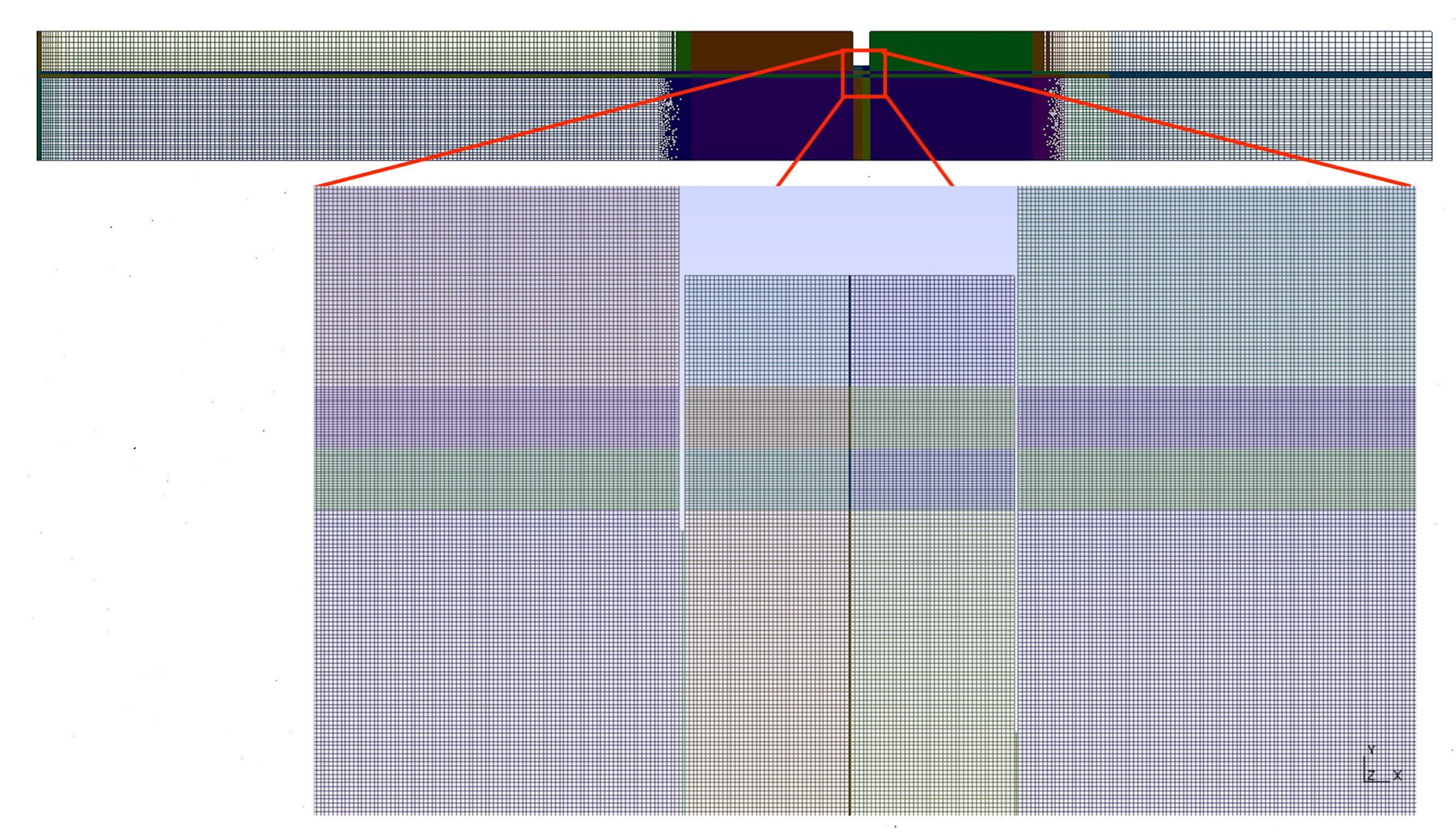
In addition to the spatial discretization tested for the wave channel, a refinement zone of two wavelengths, i.e., one wavelength to each side of the OWC, was applied to the area around the device. Inside this refinement zone, mesh elements had a horizontal and vertical size of 0.01 m, except for the slot opening region, where the horizontal size of elements were 0.0025 m. The mesh used for the study validation can be seen in
Figure 8.
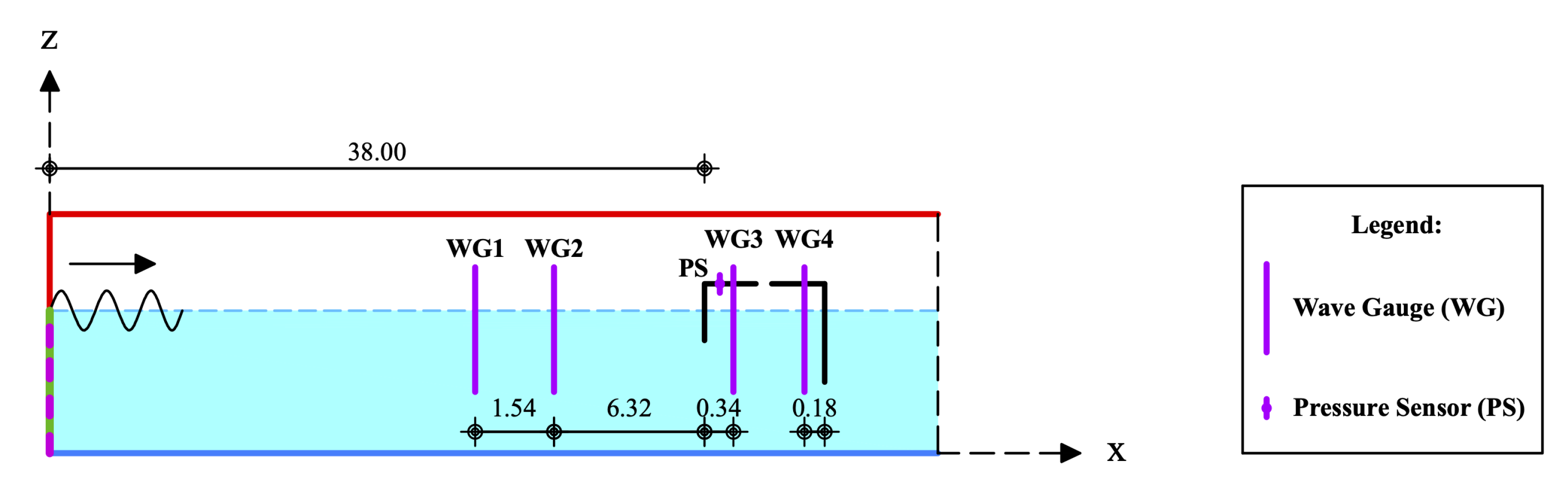
To measure water free surface elevation and air pressure, 4 numerical wave gauges (WG) and a pressure sensor (PS) were used. From these, 2 wave gauges were positioned previously to the front wall of the device and all the others were positioned inside the hydropneumatic chamber of the computational domain. The front wall of the OWC device was positioned 38 m from the beginning of the wave tank.
Figure 9 indicates the location of the sensor and gauges positioned in the chamber and along the wave tank.
In addition to spatial and temporal discretization, other numerical parameters were also defined and adopted for the verification and validation. A pressure-based solver was used for the numerical simulation. To solve the problem of linear dependence of velocity on pressure, the velocity-pressure coupling scheme pressure-implicit with splitting of operators (PISO) was adopted. A first order upwind scheme was applied for the discretization of spatial derivatives in the momentum equations, and a first order implicit formulation was adopted for time discretization. For the volume fraction, the geo-reconstruct method was applied; and for pressure interpolation at volume faces, the pressure staggering option (PRESTO!) scheme was used. In the verification simulations, only laminar flow was considered, and for the validation case two turbulence models were also considered: k- and k- shear stress transport (SST).


 ,
, 


