Design of a Marine Sediments Resistivity Measurement System Based on a Circular Permutation Electrode

Abstract

Marine sediments are rich in mineral resources, organic resources, and microbial life. The study of marine sediments is of great significance for the development and utilization of marine resources and understanding the life process. Resistivity is the overall characteristic of the electrical conductivity of marine sediments. Measuring the resistivity of marine sediments is helpful to ascertain the marine geological structure, study the distribution of marine mineral resources, and evaluate the marine soil environment. Measuring the resistivity of marine sediments is of great significance to promote marine exploration. At present, the resistivity measurement device on the market can be directly used to measure soil and water on land, but if used to measure marine sediments, it will be disturbed by seawater temperature and pressure, resulting in large errors. In this paper, a high-precision pressure-maintaining transfer system of marine sediment resistivity measurement instrument based on circular permutation electrode is designed, which can measure the resistivity of marine sediment samples after pressure-maintaining transfer. At the same time, a new type of circular permutation electrode measurement method is proposed, which makes the resistivity value more accurate, reduces the length of the probe appropriately, and saves the cost. By measuring the resistivity of marine sediments, the type of sediments can be inverted, which provides a way of thinking about the promotion of the research and development and utilization of marine resources.

1. Introduction

Marine sediments [1] are composed of insoluble materials (rocks, soil particles, etc.) transported from land to sea by wind, ice, and rivers. They also contain chemical sediments in seawater, products of submarine volcanoes, and debris of marine organisms. Marine sediments contain abundant mineral resources and organic resources, including offshore oilfields [2], sulfur, phosphate rocks, polymetallic crust, and nodules. Marine sediments are also rich in microbial life, which promotes global biomass to a large extent and is also a key component of the earth system. The study of marine sediments is of great significance in finding marine minerals, developing and utilizing marine microbial resources, studying paleoclimate evolution, understanding the formation and evolution of the ocean, and understanding the evolution and origin of life.

Resistivity is the overall characteristic of the electrical conductivity of marine sediments. Measuring the resistivity of marine sediments is of great significance for exploring marine geological structures [3], studying the distribution of marine mineral resources, and evaluating the corrosiveness of a marine soil environment. The resistivity characteristics of marine sediments are mainly affected by porosity [4], water content, hydrate saturation and sediment types, and the properties of sediments can be inverted by resistivity values. At present, the equipment for measuring the resistivity of marine sediments has not been used for commercialization and is still in its infancy. Some resistivity measurement devices are mainly used for land, such as soil and water measurement. If used to measure marine sediments, due to the interference of seawater temperature and pressure, there will be large errors. Therefore, it is not only of great scientific significance, but also of important application value to develop a marine sediment resistivity measuring instrument suitable for deep sea.

The commonly used methods for measuring the resistivity of marine sediments are mainly drag method and penetration method. Jackson [5] first developed a device to measure the resistivity of marine surface sediments. The electrode was installed on the plate, and the resistivity of marine sediments was directly measured by the dragging method, but the measurement depth was only 0.5 m. Dale F. Rucker et al. [6] used the drag method to investigate the water resistivity of sediments in the Panama Canal. In order to adapt to the required depth of investigation, the electrode spacing along the cable should reach 15 m and the total length of the cable should reach 170 m. The penetration method mainly includes the ring electrode measurement method and the point electrode measurement method. Won [7] designed a four-ring Wenner electrode resistivity measurement probe. A Rosenberger [8] designed a four-point electrode resistivity measurement probe. According to the principle of ring electrode resistivity measurement, Fu et al. [9] in 2015 designed a ring copper electrode probe with as many as 94 components of equidistant (1.0 cm apart). Three people adopted the ring electrode measurement method. The continuous ring electrode for resistivity measurement can improve the accuracy of the resistivity value by increasing the number of measurements, but it also increases the length of the probe. Therefore, this paper combines the measurement number and the length of the probe, and proposes a new circular permutation electrode method.

The resistivity meter for monitoring water quality and measuring soil has become mature, but most of the devices used in marine sediments do not consider the seawater temperature or pressure. Therefore, it is very important to design a resistivity meter for marine sediments considering seawater temperature and pressure. The accuracy of the resistivity meter for measuring soil is ±5%, and the error of the resistivity meter for measuring marine sediments will be larger, so it is also very important to improve the accuracy of the resistivity meter. In view of the lack of consideration of seawater temperature and pressure in the current resistivity meter for marine sediments, this paper designed a new type of resistivity measurement device for marine sediment samples after pressure-maintaining transfer. At the same time, the original ring electrode measurement method was improved, and a new type of circular permutation electrode measurement method was proposed. The corresponding device and probe rod were designed to avoid the influence of temperature and pressure on the resistivity value of sediments.

2. Overall System Design

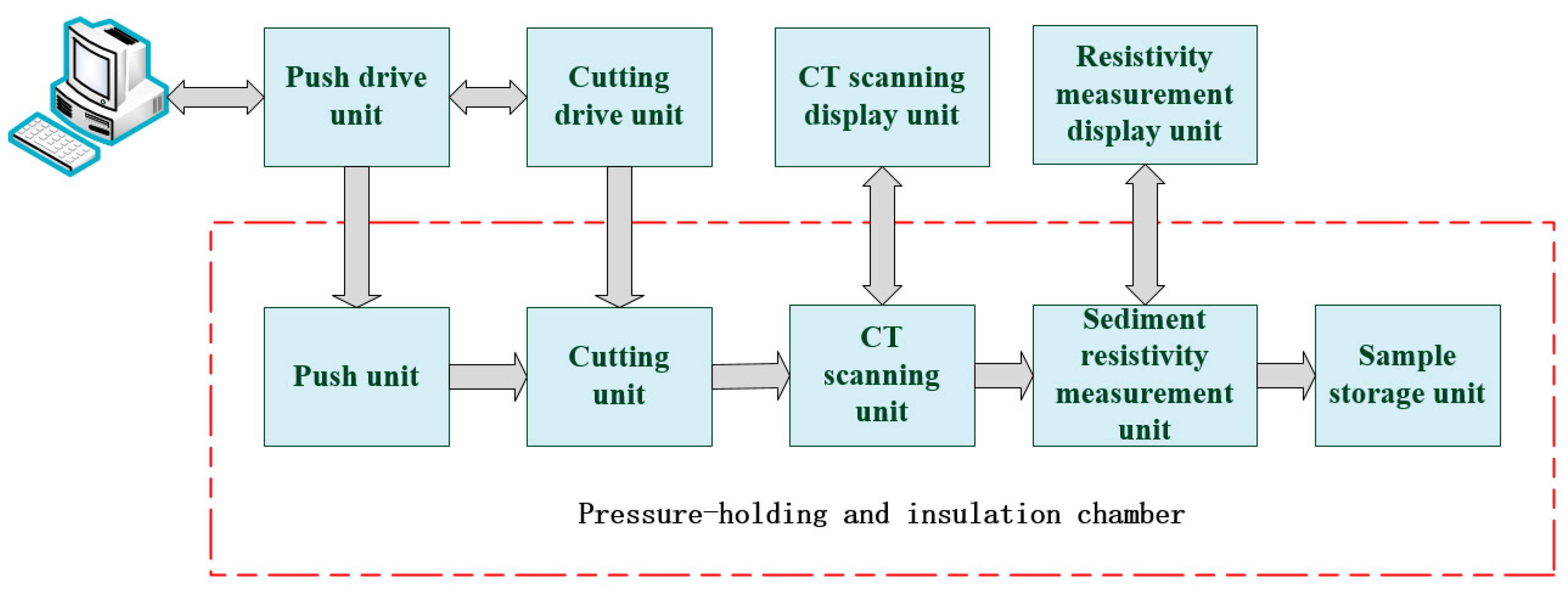
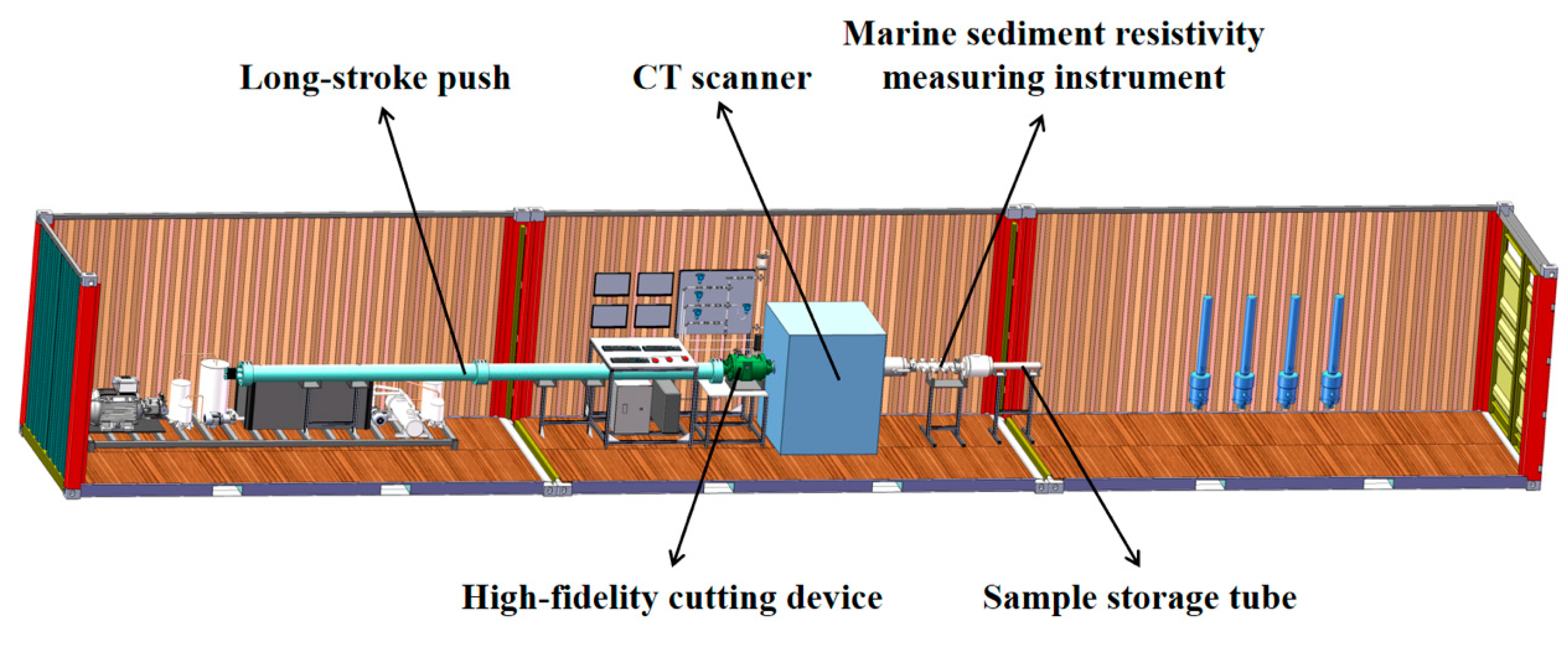
2.1. Seabed Sediment Resistivity Measuring Instrument and Marine Sediment Resistivity Measuring Instrument Pressure-Maintaining Transfer System Design

The resistivity measurement system designed in this paper is mainly used for the measurement of marine sediments after pressure-maintaining transfer. Therefore, it is necessary to consider the influence of pressure and temperature changes of sediments on the measurement results in the process of measurement. In view of this, the marine sediment resistivity measurement instrument and the pressure-maintaining transfer system of marine sediment resistivity measurement instrument are designed in this paper.

The marine sediment resistivity measuring device is shown in Figure 1. The cabin is made of 316 stainless steel. The wall thickness is 12.5 mm and the inner diameter is 65 mm, which can withstand the pressure of 36 MPa. The two ends can be connected with the pressure-maintaining transfer system of the marine sediment resistivity measuring device through the hoop. The cabin has a thread hole, which can maintain environmental pressure when measuring the resistivity of the sediment.

The detecting rod is composed of the counter–wire joint, ball valve, O-ring, thread guide rod, thread cap, thrust ball bearing, flange bearing, and elastic retaining ring. The detecting rod is connected to the cabin by the wire joint, and the ball valve control can open and close to control the penetration of the detecting rod and the cabin. O-ring is used for sealing between screw guide rod and ball valve. The thread guide rod is nested with the thread cap, and the tool or probe is rotated through the thread to enter the cabin. The upper part of the detecting rod is equipped with thrust ball bearings, flange bearings, and elastic retaining rings.

The cutting tool is made of stainless steel and adopts an integrated structure. The lower end face is machined with a cutter head. During the drilling process of the cutting tool, the plastic pipe outside the sediment sample is opened. The probe enters the sediment sample through the opening for data collection.

The probe consists of a probe rod and probe head. A POM (Polyoxymethylene) tube was selected as the shell material of probe rod. The probe rod is 360 mm in length and 10 mm in diameter. Six groups of ring electrode grooves were set on the POM tube with equal spacing. Brass was selected as the electrode material to facilitate electrode placement. A lead hole was set in each groove to facilitate electrode connection to the probe.

A principle block diagram and device diagram of pressure-maintaining transfer system of the marine sediment resistivity measuring instrument are shown in Figure 2 and Figure 3 as follows. After the pressure-maintaining transfer device obtains the marine sediment core, it is necessary to transfer the sediment core into the marine sediment resistivity measuring instrument without releasing the sediment pressure through the transfer system. The sediment is pushed backward by the long-stroke push device of the pressure maintaining core tube in the pressure-maintaining transfer system, the core samples are cut by the high-fidelity cutting device, the samples are scanned by the CT scanning device to obtain the preliminary detection results, and then the results can be compared with the measured resistivity. After the detection and processing, the sediment core is pushed into the marine sediment resistivity measuring instrument controlled by the ball valve. Firstly, the drilling device composed of the detecting rod and the cutting tool is drilled. Three test holes are drilled above the plastic tube outside the sediment core sample. The opening position of the test hole is consistent with the probe position of the three test rod devices. The resistivity test rod is moved to the pressure chamber by manual spiral propulsion, so that the probe enters the plastic tube outside the sediment core sample and extends into the drilled test hole opening to directly contact the core of the sediment for resistivity testing and data acquisition.

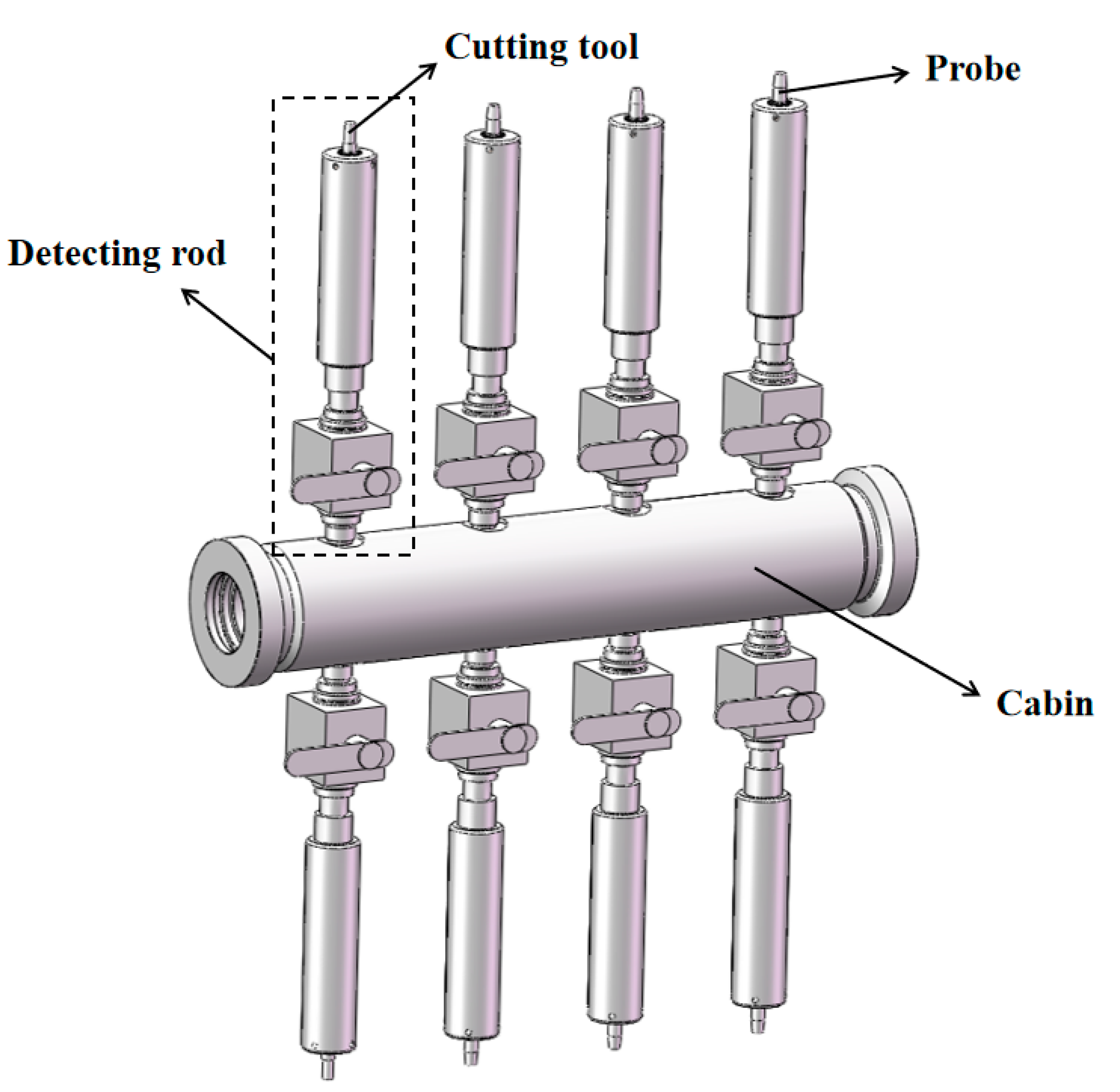
2.2. Structure Design of the Probe

POM (Polyoxymethylene) tube is selected as the probe shell material. POM is an engineering plastic with excellent performance, which has the hardness, strength, and steel properties similar to those of metals. It has good self-lubrication, fatigue resistance, and chemical resistance in a wide range of temperature and humidity. The probe consists of a probe rod and a probe head. The structure of the probe is shown in Figure 4, and the profile of the probe is shown in Figure 5. The probe rod is set to 360 mm in length and 10 mm in diameter. Six groups of ring electrode grooves are set on the probe rod with equal spacing. Brass is selected as electrode material to facilitate electrode placement. A lead hole is set in each groove to facilitate electrode connection to the probe. At the same time, in order to obtain more accurate resistivity values, this paper set up a number of different electrode spacing and electrode diameter; the first probe rod diameter was fixed at 10 mm, and then changed to different electrode diameters—1 mm, 1.2 mm, 1.4 mm, 1.6 mm, 1.8 mm, and 2.0 mm, respectively, with 0.2 mm interval, a total of 6 groups, after selecting the best electrode diameter. The probe rod diameter were then changed to 10 mm, 11 mm, 12 mm, 13 mm, 14 mm, and 15 mm, respectively, with a 1 mm interval, a total of 6 groups, to determine the best electrode diameter.

2.3. Hardware Design of the Measurement System

The overall hardware structure of the resistivity measurement system is shown in Figure 6. The hardware circuit system mainly includes a master module, squeeze module, acquisition module, communication module, storage module, power module, and temperature module. The master module is mainly responsible for controlling and processing the relevant information of each sub-module and implementing thread management. The squeeze module generates sine wave signals with different frequencies according to the command information issued by the master module and provides them to the electrode through subsequent processing and conversion. The acquisition module is responsible for collecting the weak voltage signals generated at both ends of the electrode and reporting them to the master module after processing and conversion. The communication module is responsible for the information interaction between the master module and the upper machine. The power supply module provides the required waveform stable power for the whole hardware system. The temperature module is responsible for collecting the temperature of the system to provide temperature compensation and correct the resistivity value. The storage module stores the collected data in accordance with the preset format to the SD card.

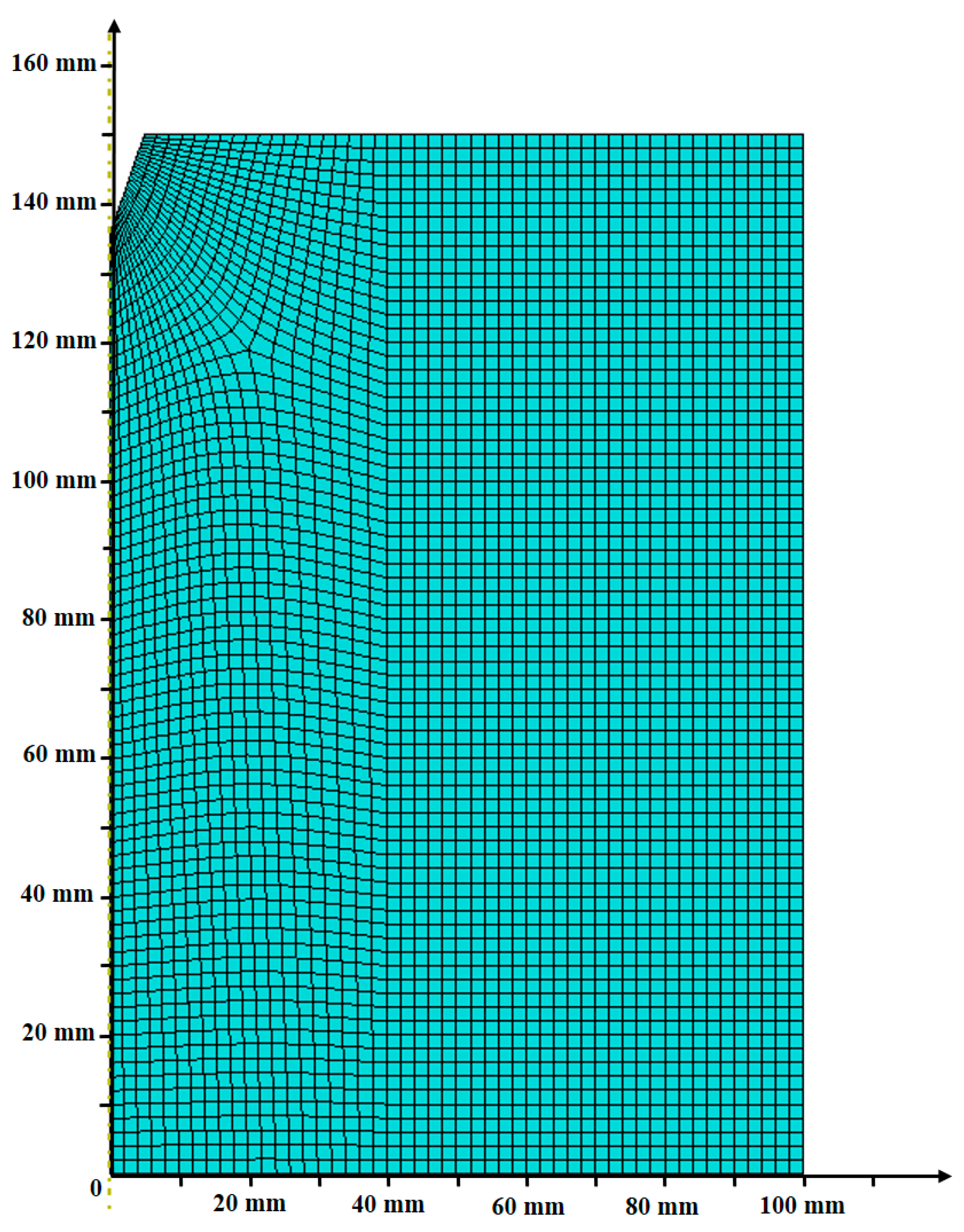
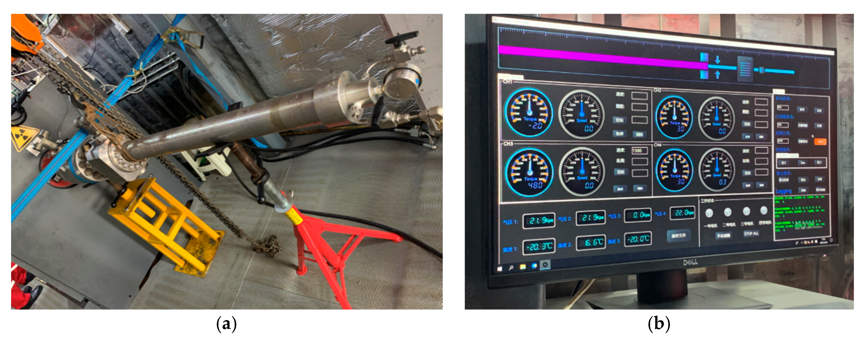
3. Mechanical Mechanism Simulation

There are many widely accepted numerical simulation methods: Lagrangian method, Eulerian method, Computational Fluid Dynamics (CFD), and Arbitrary Lagrangian–Eulerian (ALE). The Lagrangian method can accurately describe the particle motion trajectory [10], but in the calculation of such large deformation problems as the penetration soil, the excessive deformation and distortion of the grid can easily lead to the deformation of the calculation grid, and eventually lead to the difficulty of convergence [11]. The Eulerian method overcomes the Lagrangian mesh distortion problem, but the material flow at the interface is difficult to calculate, so the pure Eulerian method is not generally used to analyze the geotechnical penetration process. The Arbitrary Lagrangian_Eulerian method (ALE) combines the advantages of the Lagrangian analysis method and the Eulerian analysis method. ALE allows the grid unit to move independently of the material without changing the grid unit and connection relationship [12]. A complete ALE analysis consists of two steps: first, create a new grid, and then transfer the answers to the old grid and state variables to the new grid. Through this method, the grid and the material point can be separated from each other, so even if the grid has a large distortion, the ALE method can also ensure high quality grid throughout the analysis process. Based on the above mechanism, the finite element simulation analysis of the whole penetration process can be carried out by using the ALE method to penetrate the probe into the core sample.

In order to reduce the calculation time and improve the simulation efficiency, the dynamic implicit analysis method is adopted and the axisymmetric model is used to simulate. Probe part: POM material strength is much greater than the strength of soil, so discrete rigid body simulation is used. Soil part: the soil cylinder with the probe penetration path as the axis, the radius of 0.5 m, and the depth of 1.5 m is selected as the analysis object, and the radius of the cylinder is 50 times the cone radius. It can be considered that the boundary does not affect the stress and deformation of the soil near the axis. The position of the soil surface at the axis is reserved, and the size is the same as the probe cone size. Before penetration, the probe is placed in the opening in advance, and the probe cone tip is flat with the soil surface.

Before meshing, in order to refine the vicinity of the cone tip, the soil is first separated and meshed, respectively. The soil element type is an eight-node axisymmetric four-order displacement bilinear quadrilateral pore pressure element (CAX8P). During the penetration process, the soil has a large deformation. In order to reduce the distortion of the soil after deformation, the grid is arranged in the form of upper left to lower right, as shown in Figure 7. The analysis of the whole penetration process is shown in Figure 8.

4. Design of Resistivity Measuring Instrument

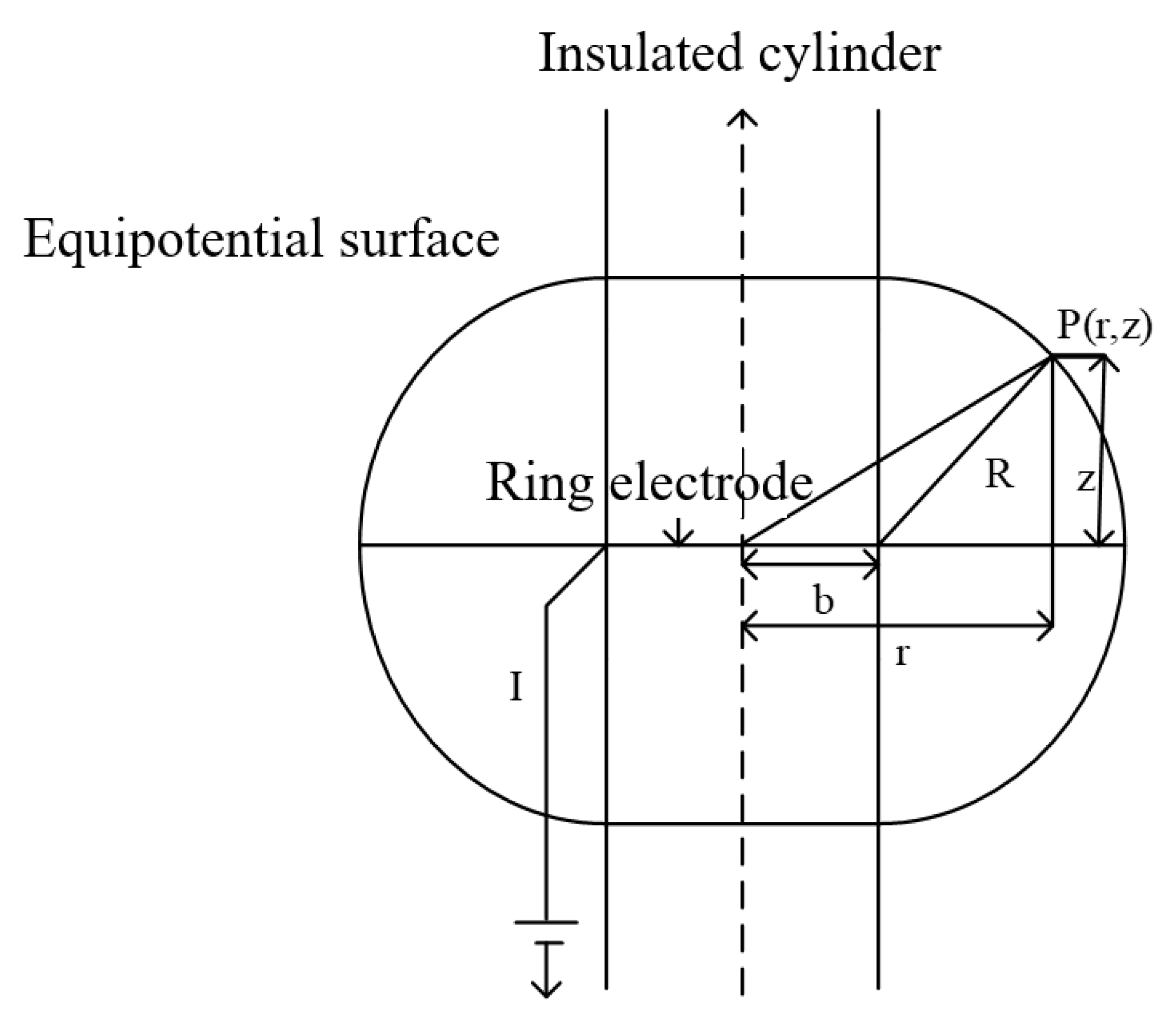
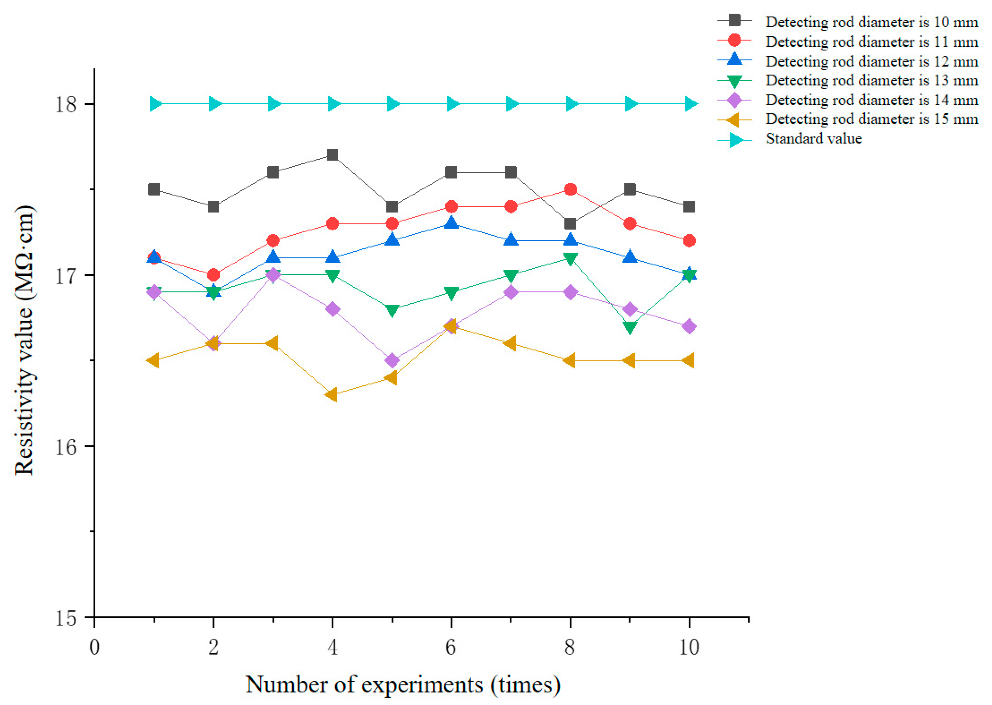
4.1. Design of Key Parameters for New Kind Circular Permutation Electrode

The ring electrode measurement method is one of the penetration measurement methods, which can directly deploy the electrode array to marine sediments. As shown in Figure 9, the ring electrode installed at a certain distance is embedded on the surface of the vertical rod. After the probe is installed, it can be measured by selecting four continuous electrodes.

Similar to the horizontal array four-electrode resistivity measurement technology, the ring-electrode resistivity measurement technology adopts the principle of the electric field of the uniform isotropic medium half-space point power supply [7]. The principle of electric field distribution is shown in Figure 10.

It can be understood that a cylinder with radius of $b$ and infinite length is embedded in a homogeneous isotropic medium. The resistivity of the medium is $\rho$. The current source connected to the annular electrode A₂ injects uniform current in its radial direction. Assuming that A₁ is at infinity, the current source will form an equipotential surface with the insulating probe rod as the boundary.

The current density at any point $p(r,z)$ on the equipotential surface is:

$$J_n=\frac{I}{4\pi R(R+\frac{\pi b}{2})}$$

(1)

In the formula $4\pi R(R+\frac{\pi b}{2})$ is the area of the circular equipotential surface, R is the distance from point P to the ring electrode, then:

$$R^2={(r-b)}^2+z^2$$

(2)

Formula (1) satisfies the boundary condition: $J_{\mathrm{n}}\approx \frac{I}{4\pi R^2}$ at infinity. The current intensity on the cylinder surface is 0, according to Ohm law:

$$J_n=\frac{1}{\rho }\frac{\partial V}{\partial R}$$

(3)

where V is the P-point potential, the Formula (1) is combined with the Formula (3) to obtain:

$$V_{\left(r,z\right)}=-\frac{I\rho }{4\pi }{\displaystyle \int \frac{\mathrm{dr}}{R(R+\frac{\pi b}{2})}}$$

(4)

Then there are:

$$V_{\left(r,z\right)}=\frac{I\rho }{2{\pi }^{2}b}\ln (1+\frac{\pi }{2}\frac{b}{\sqrt{{(r-b)}^2+z^2}})$$

(5)

$\underset{b\to 0}{{\displaystyle \lim }}V=\frac{I\rho }{4\pi R}$ is the electric potential of point source.

The Wenner ring electrode arrangement is the four electrodes arranged according to Wenner, namely equidistant vertical installation on the insulation probe surface.

According to Wenner configuration of four electrodes, external A₁ and A₂ are current source electrodes, and internal V₁ and V₂ are potential difference measurement electrodes. All electrodes are arranged in equal spacing, and the spacing is a.

The potential of V₁ is:

$$V_{V_1}=V_{A_2}\left(2a\right)-V_{A_1}\left(a\right)$$

(6)

The potential of V₂ is:

$$V_{V_2}=V_{A_2}\left(a\right)-V_{A_1}\left(2a\right)$$

(7)

According to the Formulas (5)–(7), the potential difference between V₁ and V₂ is:

$$\begin{array}{l}\Delta V=V_{V_2}-V_{V_1}\\ =\frac{I\rho }{{\pi }^{2}b}\left[\ln (1+\frac{\pi b}{2a})-\ln (1+\frac{\pi b}{4a})\right]\end{array}$$

(8)

Let resistivity $\rho$ be:

$$\rho =4\pi G\frac{\Delta V}{I}$$

(9)

The electrode geometry configuration factor G of the vertical four-ring Wenner arrangement is:

$$G=\frac{\pi b}{4}{[\ln \frac{4a+2\pi b}{4a+\pi b}]}^{-1}$$

(10)

After calculating the electrode geometry configuration factor, the resistivity $\rho$ can be calculated.

The traditional Wiener ring electrode method only uses four electrodes, which is not conducive to obtaining accurate values. Therefore, we propose a new kind circular permutation electrode measurement method, and the developed probe is shown in Figure 11.

At present, there are three methods of resistivity measurement using the C₁C₂C₃C₄, C₂C₃C₄C₅, C₃C₄C₅C₆ electrode combination. The advantage of this method is to increase the number of measurements and make the calculated value more accurate, but this will also make the probe length too long, which is not conducive to the later design. Therefore, considering the measurement times and the length of the probe, we designed a circular permutation electrode probe, that is, we can use the similar measurement of C₁C₂C₅C₆, that is, the current is injected into C₁ and C₆ to measure the potential difference between C₂ and C₅. If we design x (x > = 4) electrodes, according to the traditional method, we only have the x−3 group measurement method. If we use the new kind ring circuit measurement method, we can have $C_i^4$ kinds of measurement method, which reduces the length of the probe, saves cost, and facilitates subsequent calculation.

For example, for C₁, C₂, C₃, C₅ four electrodes have:

$$V_{C_2}=V_{C_1}(a)-V_{C_5}(3a)$$

(11)

$$V_{C_3}=V_{C_1}\left(2a\right)-V_{C_5}\left(2a\right)$$

(12)

According to Formulas (5), (11), and (12), the potential difference between C₁ and C₂ is:

$$\Delta V=\frac{I\rho }{2{\pi }^{2}b}\ln \left(\frac{6a+3\pi b}{6a+\pi b}\right)$$

(13)

For C₁, C₂, C₃, C₆ four electrodes have:

$$V_{C_2}=V_{C_1}(a)-V_{C_6}(4a)$$

(14)

$$V_{C_3}=V_{C_1}\left(2a\right)-V_{C_6}\left(3a\right)$$

(15)

According to Formulas (5), (14), and (15), the potential difference between C₁ and C₂ is:

$$\Delta V=\frac{I\rho }{2{\pi }^{2}b}\ln \left(\frac{\left(2a+\pi b\right)\left(6a+\pi b\right)}{\left(4a+\pi b\right)\left(8a+\pi b\right)}\right)$$

(16)

The electrode geometry configuration factor G of the vertical four-ring Wenner arrangement is:

$$G=\frac{\pi b}{2}{[\ln \frac{\left(2a+\pi b\right)\left(6a+\pi b\right)}{\left(4a+\pi b\right)\left(8a+\pi b\right)}]}^{-1}$$

(17)

After calculating the electrode geometry configuration factor, the resistivity $\rho$ can be calculated.

After calculating the resistivity of each electrode combination, the average value is:

$$\overline{\rho }=\frac{1}{C_x^4}{\displaystyle \sum _{i=1}^{C_x^4}{\rho }_i}$$

(18)

In this way, more accurate resistivity value can be obtained, and the length of the probe can be appropriately reduced to facilitate the subsequent design.

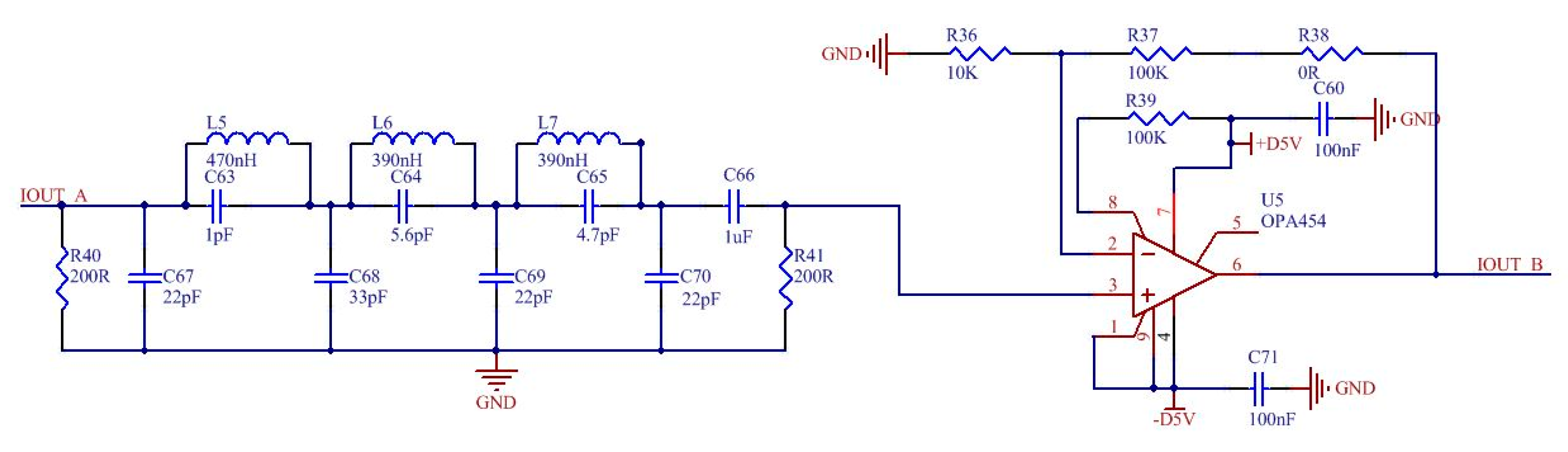
4.2. Key Parameter Design of the Filter and Amplification Module

Because DDS [13] adopts an all-digital structure, spurious is inevitably introduced. There are three main sources of error: spurious caused by phase round-off error of phase accumulator, spurious caused by amplitude quantization error as a result of limited word length of memory, and spurious caused by non-ideal characteristics of a D/A converter. Therefore, in order to obtain a better quality output signal, a low-pass filter is added to the signal output end. The main function of the filter is to filter out the high frequency noise in the output spectrum. Common types of low-pass filters include the Butterworth filter, Chebyshev filter, and elliptical filter. Among them, the transition bands of the Butterworth filter and Chebyshev filter are relatively flat, while the elliptical filter has a steep transition band, which is more suitable for filtering the noise near the passband frequency. Therefore, the elliptical filter is selected in this paper. Considering the chip output signal cut-off frequency of 70 MHZ, a low-pass elliptic filter with cut-off frequency of 70 MHZ is designed.

The order of the elliptic filter is calculated according to Matlab [14], and the calling format is as follows:

$$[n,Wp]=ellipord(Wp,Ws,Rp,Rs)$$

(19)

where n is the minimum order of elliptic filter, Wp is the cut-off angular frequency of the elliptic filter, Ws is the stopband starting angular frequency of the elliptic filter, Rp is the passband ripple, and Rs is the minimum stopband attenuation. The Filter Solution software is used to calculate the parameters of the internal components of the filter, and a 7-order elliptic low-pass filter with a cut-off frequency of 70 MHz is obtained. At the same time, due to the small output signal of AD9851 [15], the signal is amplified to the required range through the amplitude, and the amplification factor is (R₈ + R₉)/R₇. Here, OPA454 is used as the amplification chip. OPA454 is a high-voltage operational amplifier produced by TI company. Its dynamic range is 100 V, and the maximum output current is 50 mA. The filter and amplification circuit are shown in Figure 12.

4.3. Key Parameters Design of the Constant Current Source Module

Since AD9851 outputs voltage signal, if voltage power supply is adopted, the device may be damaged due to excessive current, so the power supply circuit of this system adopts a constant current source power supply. Therefore, it is necessary to convert the AC voltage signal generated by the signal generation circuit to the AC current signal, and the conversion of voltage and current is realized by the voltage control current source. Therefore, as shown in Figure 13, a voltage-current conversion circuit is designed, which is composed of a voltage follower and an in-phase summation operation circuit.

For the voltage follower:

$$U_1=U_3$$

(20)

For the in-phase summation operation circuit:

$$U_5=\frac{R_{11}}{R_{11}+R_{12}}{U}_{OUTB}+\frac{R_{11}}{R_{11}+R_{12}}{U}_3=0.5U_{OUTB}+0.5U_3$$

(21)

The output voltage U₇ is:

$$U_7=(1+\frac{R_{14}}{R_{13}})U_5=2U_5$$

(22)

Substituting Formula (22) into Formula (21), we get:

$$U_7=U_{OUTB}+U_3$$

(23)

The voltage on R₁₅ is:

$$U_{15}=U_7-U_3=U_{OUTB}$$

(24)

So the output current I_OUTC is:

$$I_{OUTC}=\frac{U_{OUTB}}{R_{15}}$$

(25)

Therefore, the output current can be adjusted by changing the value of R₁₅, and finally a sinusoidal current signal with stable waveform and constant amplitude is output.

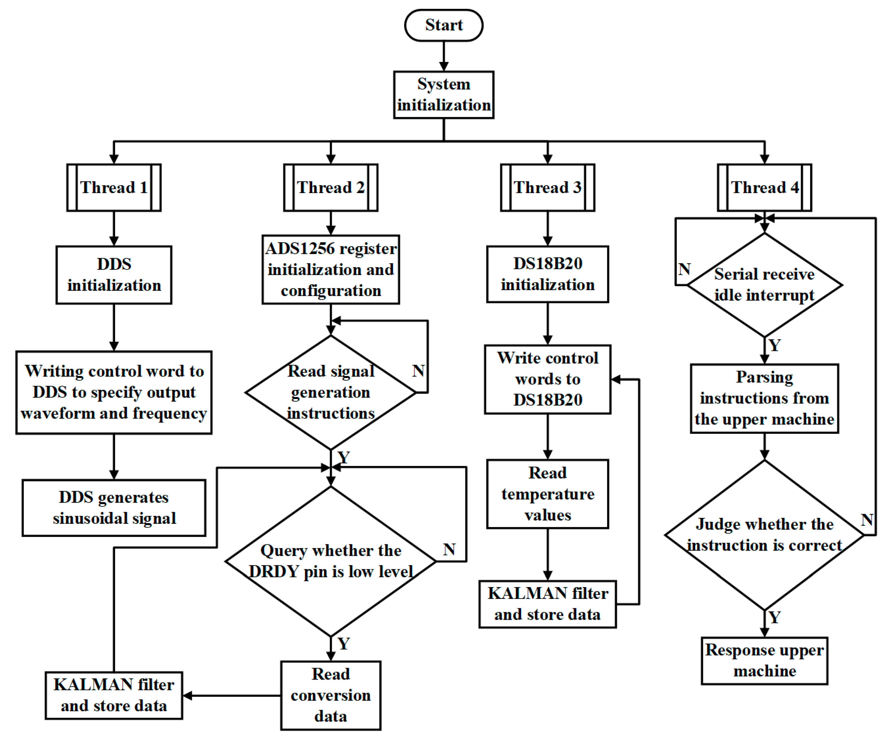
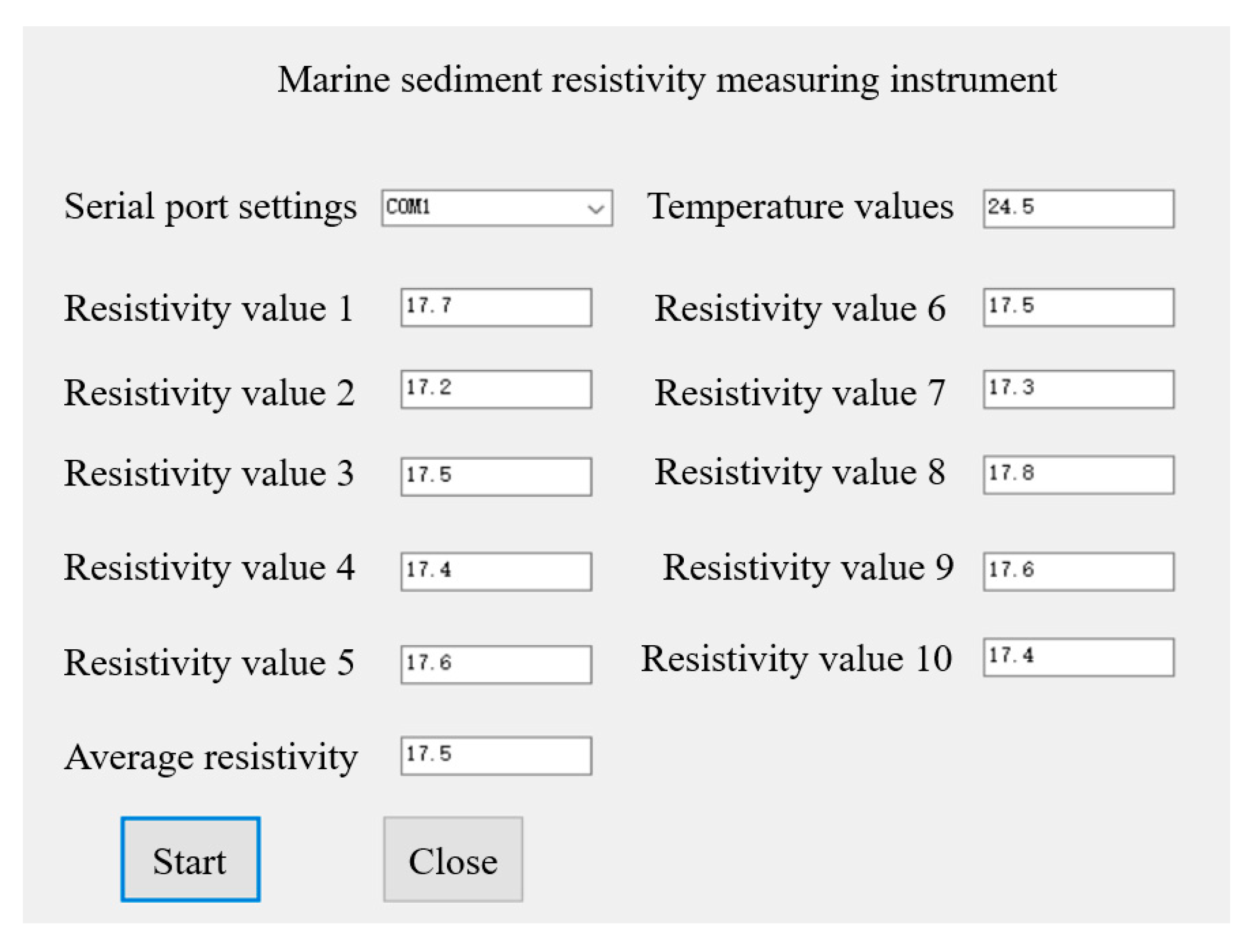
4.4. System Software Design

The system software design is mainly divided into the lower machine program design and the upper machine program design; the lower machine software design flow chart is shown in Figure 14, mainly through the Stm32Cube to build the corresponding framework, and the initialization configuration, the use of multi-threaded processing method in the system of DDS driver module, analog-to-digital conversion module, temperature acquisition module and communication module processing; at the same time, the collected voltage and temperature values are stored in the SD card after the initial Kalman filter processing and the communication module uses the serial port to receive an idle interrupt way to monitor the data sent by the upper machine and respond according to the analysis. The upper machine selects the integrated environment Visual Studio 2019 [16], based on NET Framework 4.8, and uses multi-threaded processing to process the communication module, data analysis module, and data display module in the system.

The software design flow chart of the upper machine is shown in Figure 15. After the system is initialized, the man–machine interface instruction waits to be received, and the inquiry instruction is sent to the lower machine after receiving the inquiry instruction. The data is received by the serial port in real time and judges whether it enters the interrupt function. The correct data are preprocessed, displayed, and stored, and the wrong data are discarded.

The upper machine software interface of the marine sediment resistivity measuring instrument is shown in Figure 16. After the software is opened, the circuit is connected and the serial port is set to the corresponding port number, and then clicked to start; the resistivity value of the resistivity measuring instrument can be directly measured.

5. Resistivity Measuring Instrument Experiment

Firstly, the distilled water with standard value was measured, and the appropriate electrode diameter and electrode length of the detecting rod were determined by comparing with the standard value. Secondly, the conductivity of the standard liquid was measured, and the error range was determined by comparing with the standard value. Finally, the resistivity of the marine sediments was measured.

5.1. Electrical Resistivity Measurement of Distilled Water in a Laboratory

The resistivity of the purchased industrial distilled water is 18 MΩ.cm, the electrode diameter is fixed to 1 mm, and different detecting rod diameters are changed to 10 mm, 11 mm, 12 mm, 13 mm, 14 mm, and 15 mm, respectively. The measurement results are shown in Figure 17.

It can be seen that under the same electrode condition, when the electrode length is 10 mm, the resistivity value is closer to the accurate value, so the electrode length is selected as 10 mm. Calculation error is:

$$d=\frac{\left|A-E\right|}{E}\times 100\%$$

(26)

A is the measured value, E is the standard value.

Substituting the measured value and standard value into (26), the average error is:

$$d=\frac{\left|17.5-18.0\right|}{18.0}\times 100\%=2.8\%$$

(27)

Keep the detecting rod diameter 10 mm, the electrode diameter is changed to 1.0 mm, 1.2 mm, 1.4 mm, 1.6 mm, 1.8 mm, and 2.0 mm, respectively.

The measured data are drawn by Origin software, as shown in Figure 18.

It can be seen that under the condition of equal electrode length, when the electrode diameter is 1 mm, the resistivity value is close to the real value, and it can be observed that the smaller the electrode diameter is, the smaller the error is. Due to the limitation of device and technology, it is impossible to make a smaller electrode diameter temporarily. Therefore, we choose the electrode diameter of 1 mm, and the average error is 2.7%.

5.2. Conductivity Measurement of Laboratory Standard Liquid

The EC conductivity buffer standard solution used in this experiment was purchased, and the standard values were 84 us/cm, 1413 us/cm, and 12.88 ms/cm, respectively. In order to prevent the artificial disturbance to the standard solution, the electrode of the resistivity measuring instrument was directly immersed in the standard solution, and the conductivity was measured. Since the resistivity value was measured, we only need to use 1/resistivity value, and then carry out unit conversion.

As shown in

Table 1. Laboratory standard liquid conductivity comparison table.

Conductivity/Times	1	2	3	4	5	6	7	8	9	10	Average Value
84 us/cm	83.1	82.3	81.6	80.7	83.2	83.6	81.3	82.6	81.2	83.6	82.32
1413 us/cm	1365	1383	1375	1356	1398	1385	1367	1358	1396	1353	1373.6
12.88 ms/cm	12.32	12.35	12.66	12.56	12.58	12.43	12.67	12.26	12.53	12.68	12.50

, the conductivity of three groups of different laboratory standard solutions was measured.

The average conductivity values obtained from multiple measurements of 84 us/cm, 1413 us/cm and 12,880 us/cm conductivity solutions were compared with the standard values. The average errors calculated by Formula (26) were 2%, 2.8%, and 2.9%, respectively.

5.3. Soil Resistivity Measurement

According to the different resistivity of different soils, we selected pottery clay, peat soil, black calcium soil, kaolinite clay, and loess in the middle red to measure and compare the corresponding resistivity. The soil resistivity is measured using the standard soil resistivity instrument purchased, as shown in

Table 2. Resistivity value of standard soil resistivity measurement purchased (unit: Ω·m).

Name/Times	1	2	3	4	5	6	7	8	9	10	Average Value
pottery clay	23.6	24.3	23.8	23.9	23.7	24.3	24.0	24.2	24.1	24.2	23.98
peat soil (pond silt)	83.6	82.7	83.0	82.9	82.7	83.5	83.3	82.8	82.9	83.1	83.05
black calcium soil (beach)	92.1	93.3	91.5	92.6	92.5	92.3	92.8	94.1	92.5	93.5	92.72
kaolinite clay (lakeside)	72.3	71.4	73.6	72.8	71.2	73.3	75.1	72.5	73.5	74.2	72.99
loess in the middle red	223.5	222.3	225.4	218.3	219.2	218.5	216.0	217.5	213.6	221.6	220.51

.

The resistivity measured by the actual developed resistivity measuring instrument is shown in

Table 3. The resistivity value of the developed soil resistivity measurement (unit: Ω·m).

Name/Times	1	2	3	4	5	6	7	8	9	10	Average Value
pottery clay	23.2	23.0	23.6	23.1	23.2	23.4	23.3	23.3	23.2	23.5	23.28
peat soil (pond silt)	80.8	81.3	81.2	81.2	82.0	81.3	81.0	81.4	81.5	81.3	81.30
black calcium soil (beach)	89.6	91.2	90.6	88.6	90.6	89.5	90.3	89.9	90.7	90.8	90.18
kaolinite clay (lakeside)	71.2	70.6	70.9	70.8	71.3	81.3	72.2	71.6	71.2	71.9	72.3
loess in the middle red	218.1	212.5	216.6	215.7	213.6	220.6	217.6	209.6	217.6	213.5	214.54

.

The average resistivity values measured by pottery clay, peat soil (pond silt), black calcium soil (beach), kaolinite clay (lakeside) and loess in the middle red were compared with the standard resistivity values. The average errors calculated by Formula (26) were 2.9%, 2.2%, 2.7%, 0.9% and 1.8%, respectively. The average error obtained from the experiment is within the error range of device design.

5.4. Sediment Resistivity Measurement

Since no samples of deep-sea pressure-maintaining sediments were taken, two different sites on the shore of Qizhen Lake were selected in this experiment to measure the resistivity of the sediments on the shore. The field test diagrams of the development instrument and standard instrument at site 1 of Qizhen Lake are shown in Figure 19a,b.

The resistivity and average values measured by developed and standard measuring instruments at Site 1 of Qizhen Lake are shown in

Table 4. The resistivity and average values measured by developed and standard measuring instruments at Site 1 of Qizhen Lake.

Resistivity Value/Times	1	2	3	4	5	6	7	8	9	10	Average Value
developed instrument	106.9	105.8	107.5	108.2	106.8	108.5	107.0	106.8	107.1	108.4	107.3
standard instrument	112.8	109.9	109.6	112.5	111.3	113.6	109.8	112.0	111.8	112.7	111.6

.

The average resistivity measured by the developed instrument is compared with that measured by the standard instrument. The average error calculated by Formula (26) is 3.9%.

The field test diagram of the developed instrument and standard instrument in site 2 of Qizhen Lake is shown in Figure 20a,b.

The resistivity and average values measured by developed and standard measuring instruments at Site 2 of Qizhen Lake are shown in

Table 5. The resistivity and average values measured by developed and standard measuring instruments at Site 2 of Qizhen Lake.

Resistivity Value/Times	1	2	3	4	5	6	7	8	9	10	Average Value
developed instrument	98.3	100.8	99.0	99.0	99.8	99.2	100.1	99.7	99.0	99.3	99.4
standard instrument	104.3	102.1	102.2	103.5	102.3	103.7	103.8	102.6	102.2	103.3	103.0

below.

The average resistivity measured by the developed instrument is compared with that measured by the standard instrument. The average error calculated by Formula (26) is 3.5%.

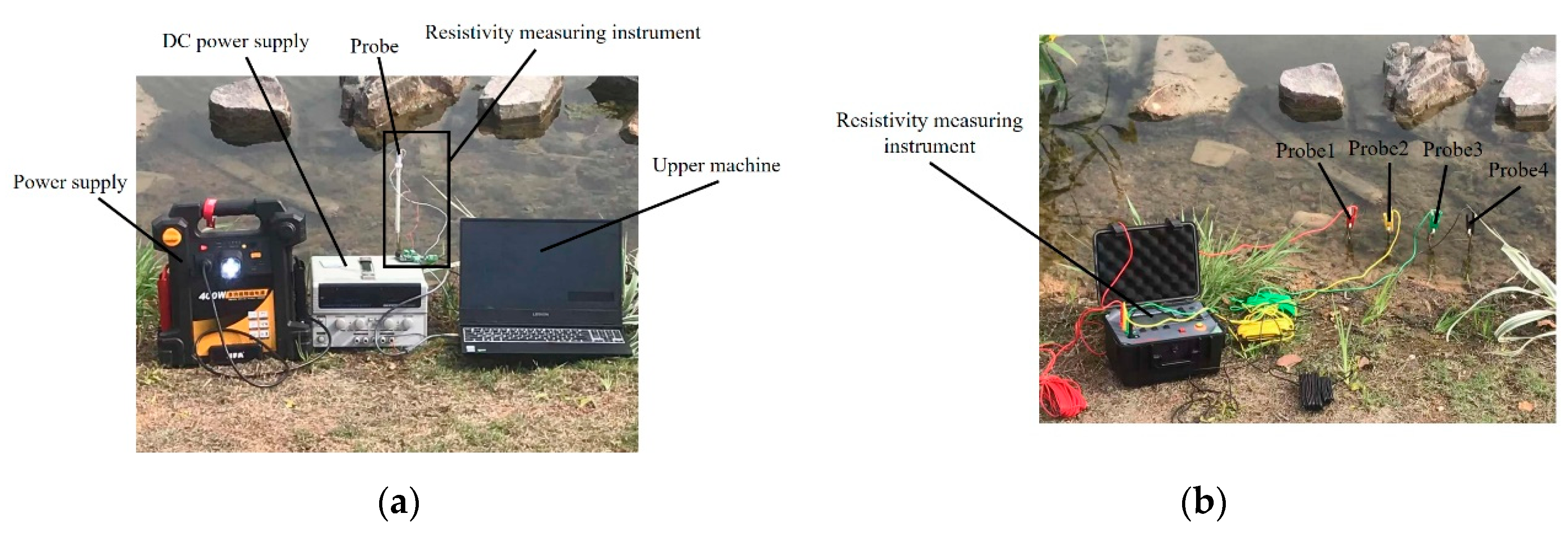
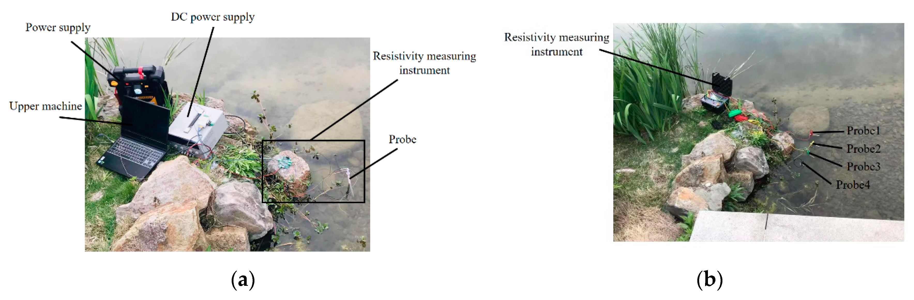
6. Overall Experiment

In order to verify the overall working performance of the marine sediment resistivity measuring instrument, the core management pressure-maintaining transfer device equipped with the system in the <Research and Application of Gas Hydrate Subsea Drilling and Shipborne Detection Technology> project was carried out in April 2021 with the No. 2 mother ship of the Guanghai Bureau of the China Geological Survey to the Shenhu area of the South China Sea for sea trial function verification.

After reaching the intended sea area, the seabed sediment was first drilled by the ‘Hainiu’ pressure-maintaining rig, and then the pressure-maintaining core tube was drilled on the shore by the rig. After the pressure monitoring met the pressure-maintaining index, it was docked with the pressure-maintaining transfer device of the shipborne core tube. As shown in Figure 21 below, after successful docking, the samples of the pressure-maintaining core tube were scanned by acoustic wave, CT scan, cutting and segmented pressure-maintaining encapsulation according to the preset control program of the pressure-maintaining transfer system.

The sample sediments containing natural gas hydrate were selected from the data results of high-fidelity cutting and CT scanning, and transferred to the marine sediment resistivity measuring instrument system connected with the pressure-maintaining transfer device. As shown in Figure 22, the resistivity measurement of transferred sediment samples was carried out by the resistivity measuring device inserted into the marine sediment resistivity measuring instrument system.

According to the preliminary scanning results, marine sediment samples containing natural gas hydrate were selected and measured by a self-made resistivity measuring instrument. A total of three sections of sediment sample tubes were selected for the measurement, and each section of sediment sample was measured five times. The data are shown in

Table 6. The resistivity measurement value (unit: kΩ·m) of the developed instrument for hydrate sediments in Shenhu Sea, South China Sea.

Resistivity Value/Times	1	2	3	4	5	Average Value
Sediment sample tube 1	7.8	7.6	8.2	7.9	7.9	7.8
Hydrate content	***	****	**	***	***
Sediment sample tube 2	7.6	7.6	8.0	8.4	8.1	7.9
Hydrate content	****	****	***	none	**
Sediment sample tube 3	8.0	7.8	7.8	8.2	8.4	8.0
Hydrate content	***	****	****	**	none

Description: * Represents gas hydrate content.

. After average calculation, and compared with the resistivity value of marine natural gas hydrate recorded in the previous literature, the CT scanner shows that the resistivity value of sediments in the area with high hydrate content is significantly lower than that in the area with low hydrate content, and it is obviously observed that the resistivity value of the area containing natural gas hydrate is lower than that of the area without natural gas hydrate.

7. Conclusions and Foresight

In this paper, a new type of resistivity measurement method based on circular permutation electrode is proposed in the design of marine sediment resistivity measurement system. In the same detecting rod length, the measurement method can carry out more measurements and reduce the error to less than 4% through the selection of components and circuit design, which is better than 5% accuracy of some resistivity measuring instruments on the market when measuring soil. At the same time, the system also includes a set of instrument pressure test cabin suitable for deep-sea sediment resistivity measurement. The cabin takes into account the influence of temperature and pressure on the measurement results. When using this cabin to implement the resistivity measurement of marine sediment under high pressure, the pressure and temperature values of the measured sediment in situ are maintained, and the accuracy of the measurement is improved. By comparing the measured results with the CT scanning results, it is found that the content of hydrate in sediments is inversely proportional to the resistivity of sediments, and the measured resistivity of sediments without hydrate has little change, which is basically consistent with the existing literature data. The subsequent research will focus on the inversion of the composition and content of the sediment through the resistivity value. At the same time, the porosity sensor, penetration force sensor and shear force sensor are embedded in the measurement system to explore the relationship between the composition and content of the sediment and each parameter.

References

1. Näslund, J. The Importance of Biodiversity for Ecosystem Processes in Sediments: Experimental Examples from the Baltic Sea. Ph.D. Thesis, Department of Systems Ecology, Stockholm University, Stockholm, Sweden, 2010. [Google Scholar]
2. Guan, Y.; Sun, X.; Ren, Y. Mineralogy, geochemistry and genesis of the polymetallic crusts and nodules from the South China Sea. Ore Geol. Rev. 2017, 89, 206–227. [Google Scholar] [CrossRef]
3. Romoen, M.; Pfaffhuber, A.A.; Karlsrud, K.; Helle, T.E. Resistivity on Marine Sediments Retrieved from RCPTU-Soundings: A Norwegian Case Study. In Proceedings of the 2nd International Symposium on Cone Penetration Testing, Huntington Beach, CA, USA, 9–11 May 2010; Volume 2, pp. 289–296. [Google Scholar]
4. Oh, M.; Kim, Y.; Park, J. Factors affecting the complex permittivity spectrum of soil at a low frequency range of 1 kHz–10 MHz. Environ. Geol. 2007, 51, 821–833. [Google Scholar] [CrossRef]
5. Jackson, P.D. An electrical resistivity method for evaluating the in-situ porosity of clean marine sands. Mar. Georesour. Geotechnol. 1975, 1, 91–115. [Google Scholar] [CrossRef]
6. Rucker, D.F.; Noonan, G.E.; Greenwood, W.J. Electrical resistivity in support of geological mapping along the Panama Canal. Eng. Geol. 2011, 117, 121–133. [Google Scholar] [CrossRef]
7. Won, I. The geometrical factor of a marine resistivity probe with four ring electrodes. IEEE J. Ocean. Eng. 1987, 12, 301–303. [Google Scholar] [CrossRef]
8. Rosenberger, A.; Weidelt, P.; Spindeldreher, C.; Heesemann, B.; Villinger, H. Design and application of a new free fall in situ resistivity probe for marine deep water sediments. Mar. Geol. 1999, 160, 327–337. [Google Scholar] [CrossRef]
9. Fu, T.; Yu, H.; Jia, Y.; Xu, X.; Guo, L. Application of an In Situ Electrical Resistivity Device to Monitor Water and Salt Transport in Shandong Coastal Saline Soil. Arab. J. Sci. Eng. 2015, 40, 1907–1915. [Google Scholar] [CrossRef]
10. Wess, J.; Bruno, Z. Lagrangian method for chiral symmetries. Phys. Rev. 1967, 163, 17–27. [Google Scholar] [CrossRef]
11. Hirt, C.W.; Cook, J.L.; Butler, T.D. A Lagrangian method for calculating the dynamics of an incompressible fluid with free surface. J. Comput. Phys. 1970, 5, 103–124. [Google Scholar] [CrossRef]
12. Hirt, C.W.; Amsden, A.A.; Cook, J.L. An arbitrary Lagrangian-Eulerian computing method for all flow speeds. J. Comput. Phys. 1974, 14, 227–253. [Google Scholar] [CrossRef]
13. Raptakis, A.; Oustoglou, C.; Sotiriadis, P.P. Laboratory Jitter Removal Circuit for Single-Bit All-Digital Frequency Synthesis. In Proceedings of the 2017 Panhellenic Conference on Electronics and Telecommunications (PACET), Xanthi, Greece, 17–18 November 2017. [Google Scholar]
14. Podder, P.; Hasan, M.; Islam, M.; Sayeed, M. Design and implementation of Butterworth, Chebyshev-I and elliptic filter for speech signal analysis. arXiv 2020, arXiv:2002.03130. [Google Scholar] [CrossRef]
15. Han, Y.K.; Suo, X.S. Design of High Precision Current Signal Source on DDS. In Proceedings of the Atlantis Press, National Conference on Electrical, Electronics and Computer Engineering, Xi’an, China, 12 December 2015. [Google Scholar]
16. Strauss, D. Getting to Know Visual Studio 2019, 3rd ed.; Apress: Berkeley, CA, USA, 2020; pp. 1–60. [Google Scholar]
Figure 1. Marine sediment resistivity measuring instrument.
Jmse 09 00995 g001
Figure 2. Principle block diagram of the marine sediment resistivity measuring instrument.
Jmse 09 00995 g002
Figure 3. Pressure-maintaining transfer system of the marine sediment resistivity measuring instrument.
Jmse 09 00995 g003
Figure 4. The probe.
Jmse 09 00995 g004
Figure 5. The probe profile diagram.
Jmse 09 00995 g005
Figure 6. The overall hardware structure of the resistivity measurement system.
Jmse 09 00995 g006
Figure 7. Diagram of grid division.
Jmse 09 00995 g007
Figure 8. Analysis diagram of the probe penetration process.
Jmse 09 00995 g008
Figure 9. Ring electrode measuring probe. Where a is the distance between the two electrodes, and b is the radius of the probe rod.
Jmse 09 00995 g009
Figure 10. Electric field distribution principle of the ring electrode.
Jmse 09 00995 g010
Figure 11. Multi-electrode ring probe.
Jmse 09 00995 g011
Figure 12. Filter and amplification circuit design.
Jmse 09 00995 g012
Figure 13. Constant current source circuit design.
Jmse 09 00995 g013
Figure 14. Software design flow chart of lower machine.
Jmse 09 00995 g014
Figure 15. Software design flow chart of the upper machine.
Jmse 09 00995 g015
Figure 16. Upper machine software interface of the marine sediment resistivity measuring instrument.
Jmse 09 00995 g016
Figure 17. Experimental plot of distilled water with equal electrode diameter and different detecting rod diameter.
Jmse 09 00995 g017
Figure 18. Experimental plot of distilled water with equal electrode diameter and different electrode length.
Jmse 09 00995 g018
Figure 19. Site 1 of Qizhen Lake developed instrument (a) standard instrument; (b) field test diagram (unit: Ω·m).
Jmse 09 00995 g019
Figure 20. Site 2 of Qizhen Lake developed instrument (a) standard instrument; (b) field test diagram (unit: Ω·m).
Jmse 09 00995 g020
Figure 21. Experimental scene diagram: (a) Equipment diagram of experimental scene; (b) The data display diagram of the experimental scene; (c) Experimental scene operation diagram.
Jmse 09 00995 g021aJmse 09 00995 g021b
Figure 22. Field plot of pressure-maintaining transfer device for marine sediment resistivity measuring instrument.
Jmse 09 00995 g022