Article

Happiness versus the Environment—A Case Study of Australian Lifestyles

by
Manfred Lenzen
1,* and
Robert A. Cummins
2
1
ISA, School of Physics A28, The University of Sydney NSW 2006, Australia
2
School of Psychology, Deakin University, 221 Burwood Hwy, Melbourne Vic 3125, Australia
*
Author to whom correspondence should be addressed.
Challenges 2013, 4(1), 56-74; https://doi.org/10.3390/challe4010056
Submission received: 19 March 2013 / Revised: 4 April 2013 / Accepted: 9 April 2013 / Published: 2 May 2013
(This article belongs to the Special Issue Challenges in Industrial Ecology)

Abstract

:
Crafting environmental policies that at the same time enhance, or at least not reduce people’s wellbeing, is crucial for the success of government action aimed at mitigating environmental impact. However, there does not yet exist any survey that refers to one and the same population, and that allows the identifying relationships and trade-offs between subjective wellbeing and the complete environmental impact of households. In order to circumvent the lack of comprehensive survey information, we attempt to integrate two separate survey databases, and describe the challenges associated with this integration. Our results indicate that carbon footprints are likely to increase, but wellbeing levels off with increasing income. Living together with people is likely to create a win-win situation where both climate and wellbeing benefit. Car ownership obviously creates emissions, however personal car ownership enhances subjective wellbeing, but living in an area with high car ownership decreases subjective wellbeing. Finally, gaining educational qualifications is linked with increased emissions. These results indicate that policy-making is challenged in striking a wise balance between individual convenience and the common good.

1. Introduction

This article follows up from a concept note [1] in which we argued that dimensions of subjective wellbeing should be connected to Industrial Ecology studies of households, in a way that such research can become more interdisciplinary, broaden its scope, and thus enhance its policy relevance. Considering the importance of the subjective wellbeing (SWB) of populations and the mitigation of environmental pollution, there is a dearth of information on the connection between the two [2]. One reason is the very different disciplines that concern each form of measurement. The former is the province of the social sciences, the latter the province of the physical sciences. Bringing these two areas together presents formidable conceptual and technical barriers.
There are several studies focussing on the relationship between wellbeing and attitudes towards the environment [2,3,4], between wellbeing and the measured state of the environment in the vicinity of the household 1, and between attitudes towards the environment and environmental impact ([8], see a comprehensive listing in [9]). Zidanšek [10] and nef [11] report on the level of happiness and environmental sustainability/footprint over time at the national level 2, however, these studies do not contain socio-economic-demographic variables that may explain common underlying traits. There are also studies focusing on environmental impact, with reference to income, human development index, human needs, and socio-economic variables, notably by Steinberger, Jackson, Druckman and colleagues [14,15,16,17,18,19,20,21,22,23], however these studies do not include measures of subjective wellbeing. Similarly, there are studies focusing on wellbeing, notably with reference to income, but excluding environmental impact [24,25].
In order to enable the investigation of relationships between wellbeing and the complete carbon footprint of households, a single database including wellbeing variables as well as household expenditure on commodities is required. We use the term “complete” to mean that all ripple effects of households’ purchasing activities are covered in the assessment [26]. It is important to use footprints, because direct, on-premises effects such as electricity and gas use in the household, or petrol use in the car, will significantly underestimate the true impact of households [27], and therefore confound conclusions about the link between wellbeing and emissions.
The relationship between SWB and emissions on one hand, and explanatory variables on the other, could in principle be derived from a range of separately published studies. However, the explanatory variables assessed in these studies are likely to differ with regard to their definitions, and the studies will most certainly refer to different populations. Therefore, one could strictly speaking not draw conclusions about the influence of certain socio-economic determinants on SWB and emissions simultaneously. This is the core issue addressed in this paper. To our knowledge, there exist at present no survey data, and hence also no assessment, in which SWB and carbon footprint of household consumption can be investigated for one and the same population, referring to one and the same set of accompanying socio-economic variables. This is remarkable, given that understanding about joint determinants of increased wellbeing and reduced carbon footprint is crucial for the design of environmental policies that are likely to be well received by the general public because of their double dividends for environment and wellbeing.
The collection of data using a survey designed to verify or falsify an a-priori formulated hypothesis is expensive and time-consuming. Rather than waiting for such survey data to become available, the work reported here integrates two existing separate databases in order to shed some light on possible determinants that are common to both personal wellbeing and the carbon footprint of consumption. When dealing with the challenge of integrating two separate databases, one necessarily has to make concessions with regard to matching their respective statistical properties, variable definitions, and populations. Our aims in this paper are (a) to describe the challenges arising out of those concessions, and (b) to arrive at indicative results that point at determinants of wellbeing and emissions that are potentially important for policy-making. The work reported here is essentially data-driven, and not theory-driven. Our aims are therefore not to offer, or prove or disprove through interpretation of results, plausible theories explaining the relationship between wellbeing and environmental impact.
First we will provide introductory definitions and a literature review for the two variable domains we are dealing with: subjective wellbeing and carbon footprint. In Section 2 we explain in detail the challenges we encountered during our data analysis, with indicative results presented in Section 2.4. The results are discussed, and the paper concluded, in Section 3.

1.1. Review of Subjective Wellbeing and Carbon Footprint

1.1.1. Subjective Wellbeing

In Australia, information on Subjective Wellbeing (SWB) gathered several times a year by the Australian Unity Wellbeing Index survey [28]. Each survey involves a telephone interview of 2,000 new respondents, nationwide. The project commenced in April 2001 and the accumulated data from the 25 surveys conducted to April 2011 have been gathered from 50,000 respondents.
The scale used to measure and conceptualize SWB is the Personal Wellbeing [29], which is designed as the first-level deconstruction of the highly abstract question ‘How satisfied are you with your life as a whole’. In order to achieve this design aim, each of the seven items has two important characteristics. The first is the semi-abstract nature of each question, such as ‘How satisfied are you with your relationships’. This format is deliberately non-specific. It allows the response that people give to be dominated by non-specific mood affect (the essence of SWB, [30]), slightly flavoured with cognitions attached to personal relationships (for the use of affect as information see [31,32]). A more specific question, such as ‘How satisfied are you with your friends’, would elicit a more cognitively driven response. The second characteristic of the seven items (domains) that comprise the Personal Wellbeing Index is that when they are together regressed against ‘Satisfaction with life as a whole’, each one contributes unique variance.
Each item is rated on an end-defined 0–10 scale [33] that is anchored by ‘completely dissatisfied’ and ‘completely satisfied’ (see [34] for an argument as to why this form of scale is superior to a Likert scale). The data are then averaged across the seven domains for each respondent and the result transformed onto a 0–100 scale. In addition to measuring SWB, the Australian Unity Wellbeing Surveys also includes socio-economic and demographic information. These companion data are used to link the two data sets (see Section 2 and Appendices).

1.1.2. Carbon Footprint

There is a long-standing tradition of investigating the environmental and resource impacts of households. The methods used in this stream of research were forged in the 1970s [35], and are still being adhered to today. Overviews of such studies are given by Lenzen et al. [36] and Hertwich [37], and we refer the reader to these articles for information beyond the brief outline given here.
In essence, an analysis of a household’s carbon footprint can be undertaken by a number of life-cycle approaches [38,39]. The approach we are applying here uses three data sources; a household expenditure database, input-output tables, and matching satellite accounts containing environmental data. In our case, these data sources are the Australian Household Expenditure Survey [40], the Australian Input-Output Tables [41], as well as four satellite accounts. These data sources are integrated via a set of equations from economic input-output theory, and yield carbon footprints as described in Appendix A.1. When using input-output tables, carbon footprints are quantified in a complete upstream life-cycle perspective, that is, covering the entire industrial supply-chain network that underpins the purchases of households.
In Australia, published satellite accounts are not harmonised with input-output tables. Thus, labour-intensive re-classification and alignment has to be carried out by the researcher. In our case, we constructed harmonised satellite accounts for the following four environmental indicators: greenhouse gas emissions [42], water use [43], land use [44], and material flow ([45] and other sources, see [46]). For an overview of the definitions and data sources underpinning the four satellite accounts see [47].

2. Challenges in Data Preparation

Our main aim is to identify possible determinants common to two key dependent variables—SWB and carbon footprint. Given the lack of a single survey containing both variables, our approach is based on two survey sources: the Australian Unity Wellbeing Surveys (AUWS, [48]; [28]), and the Australian Household Expenditure Survey (HES, [40]). The main challenge in integrating these two surveys is that they were undertaken on different samples of the Australian population, and hence cannot be combined into one file. Our strategy was therefore to utilise multiple regression and hypothesis testing in order to separately extract trends from both surveys, but on the basis of a common underlying set of determinants

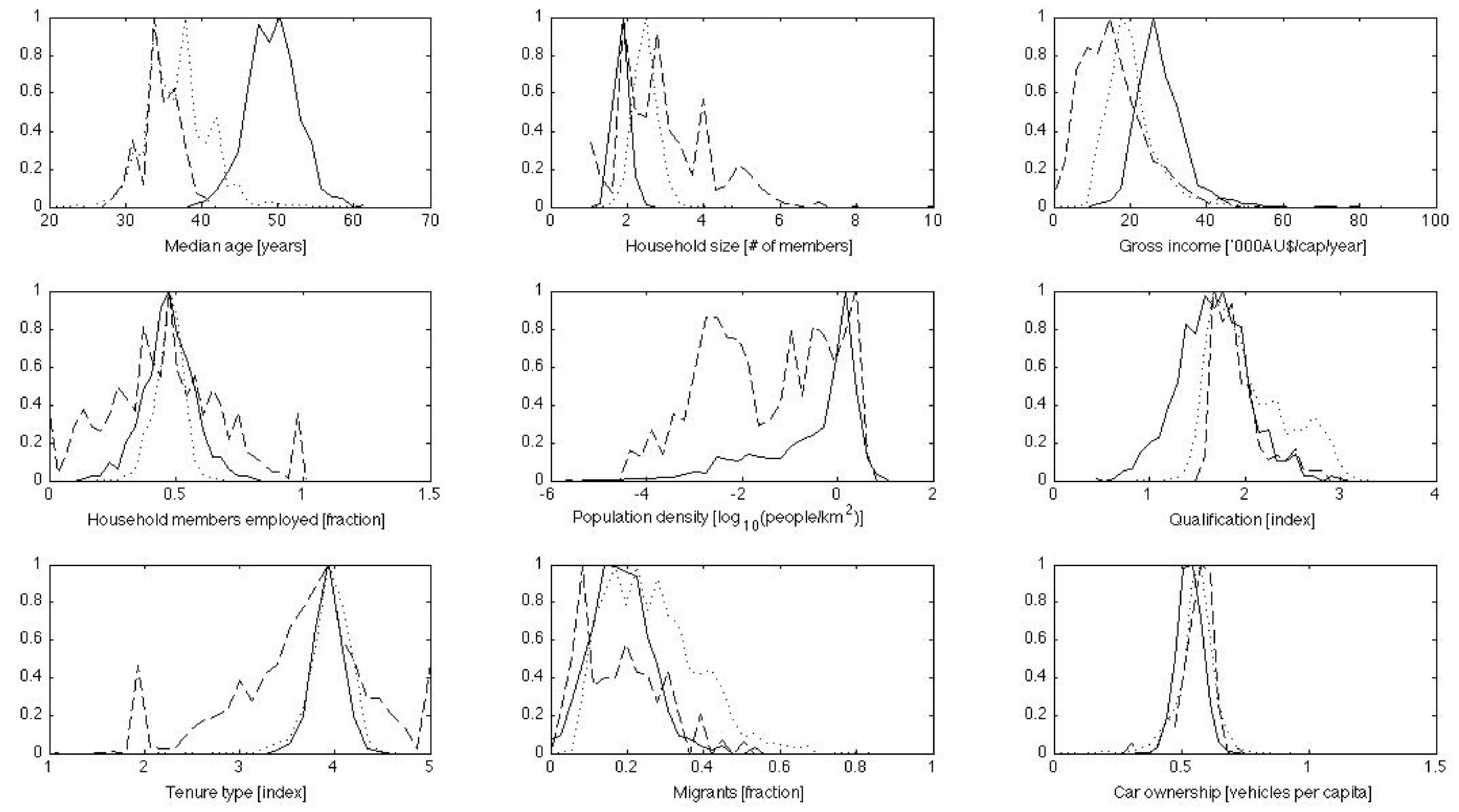
2.1. Challenge 1: Constructing a Common and Comparable Set of Explanatory Variables

Both the AUWS and HES surveys contain a range of companion data—mostly socio-economic-demographic quantities, such as employment status, income, and age—from which such a common set of explanatory variables can be derived. We were able to construct 17 such explanatory variables common to both surveys.
The companion data in the AUWS and HES are only partly overlapping, and almost never represent variables with exactly matching definitions. As a consequence, we were not in a position to extract and appraise data on variables that are intuitive candidates for explaining carbon footprint and/or wellbeing, but instead we had to follow a data-driven strategy where we essentially took whatever information was available, and examined this information for its explanatory power. A number of adjustments had to be made to the companion data in order to extract as many common explanatory variables from the two databases as could be achieved, and to align these as much as possible in terms of their definitions.
Figure 1. Normalised frequency distributions of explanatory variables (Australian Unity Wellbeing Surveys (AUWS) samples aggregated). Solid: AUWS, before filling in of missing data; dashed: Australian Household Expenditure Survey (HES); dotted: Census.
Challenges 04 00056 g001
For example, whilst the AUWS reports gross household income, the HES reports disposable (cash) income, which had to be converted into gross income using additional information on income tax payments. Similarly, the AUWS only contains the age of the survey participants, and lists the age of other household members in less than 20% of samples (most of which are households with more than 2 members). We calculated the median age for all 2-member households by (a) extracting data on those households where the age of both members were given (1.7% of samples), (b) determining from those an average ratio of median ages to respondents’ ages, and (c) applying this ratio to 2-member households where only the age of the survey participant was given. Finally, car ownership in the AUWS is queried by a simple yes/no question. In affirmative cases, we determined the number of vehicles per-capita simply by assuming one car for the entire household, and dividing by the number of household members. We suspected that this procedure could underestimate car ownership, since we miss all second vehicles. However, a comparison with Australian Census data (see Figure 1) showed that when averaged out, our car ownership variable so constructed agreed well with Census information, presumably because the majority of AUWS respondents only had one car. Subject to these adjustments, we were able to construct 17 explanatory variables common to both AUWS and HES (Table 1 and Appendix A2).
Table 1. Explanatory variables derived from companion data common to all surveys. There are 17 variables in total—9 socioeconomic-demographic variables, and 8 State dummy variables. The table describes how variables were constructed from raw data; Challenges 04 00056 i001 indicates that variable exists as raw data item. In addition, the AUWS coverage indicates what percentage of missing data had to be filled with Census information. PA = Postal Area, SD = Statistical Division, SSD = Statistical Sub-Division.
VariableDefinitionAUWS Challenges 04 00056 i002 HESCensus
(symbol)construction (see Table A1)coverage (see Table A3.2)
ageMedian age of household membersconstructed from 11 AUWS items97.7%weighted average over age ranges Challenges 04 00056 i001 (B02)
sizeNumber of household membersconstructed from 5 AUWS items66.6% Challenges 04 00056 i001 Challenges 04 00056 i001 (B02)
incAnnual per-capita gross household incomepartly directly measured, partly derived from ranges58.1%add weekly net income and income tax data Challenges 04 00056 i001 (B02)
empEmployment status—% of household members employedfull-time—100%, part-time—50%46.8%divide employed members by sizedivide labour force (B041) by population (B01)
popPopulation density—people/km2from PA Census99.9%from SD and SSD Censusdivide area (cover sheet) by population (B01)
qualQualification index (Table A2.2a)from 3 AUWS items (Table A2.2b)5.5%directly from HES (see Table A2.2a)weighted average over qualification (B39) with weights as in Table A2.2a
tenTenure type index (Table A2.3a)from 3 AUWS items (Table A2.3b)10.2%directly from HES (see Table A2.3aweighted average over tenure type (B32) with weights as in Table A2.3a
bornMigrants—% of household members born overseasborn in Australia—0, otherwise—118.3%all from Census1 – people born in Australia (B09) divided by population (B01)
carCar ownership—number of vehicles per personyes—1/size, no—08.2%all from Censusweighted average over car ownership ranges (B29)
stateState in which household is located—8 dummy variablesfrom PA code100%from SD and SSD identifiernot needed since AUWS and HES complete
The companion data in the AUWS and the HES are incomplete. The HES does not provide any information on population density, percentage of household members born overseas, and car ownership, but the 108 samples are complete with respect to the remaining variables (see details in Appendix A3). We therefore substituted missing ABWS and HES data with information from the Australian Census (Table A3.2). This is a valid procedure for the HES in any case, because Census data can be sourced from Census Basic Community Profiles for Statistical Divisions (SDs) for all HES samples and Statistical Sub-Divisions (SSDs) for HES urban area samples. The AUWS lists Postal Area (PA) code, and hence missing data were substituted from Census Basic Community Profiles for PAs. The variables where most information is complemented by Census data are “Car ownership” and “Migrants”. Hence, we must interpret these variables only to a minor extent as “car ownership in the household” or “migrant proportion in the household”, but mainly as “general car ownership in the area of residence” or “migrant proportion in the area of residence”.

2.2. Challenge 2: Matching Sample Populations

In order to compare AUWS and HES samples, together with the Census data, in terms of their mean characteristics, we aggregated the AUWS sample into random groups of 50 respondents, and re-plotted the frequency distributions (Figure 1). The AUWS respondents were on average older and richer than people in their PAs, SDs and SSDs, and lived in smaller and more urban households. However, they had similar employment status, qualification, tenure, migrant status, and car ownership. Data on population density are not contained in either AUWS or HES, but were derived from Census PAs, SDs and SSDs. The AUWS distribution of population densities is identical to, and overlaps perfectly with, the distribution of Census data for this variable.
We performed a Chow test in order to quantitatively test whether the AUWS and HES samples can be regarded as stemming from the same population. As could be expected from the distributions shown in Figure 1, this test failed, and in fact the AUWS and HES samples are different. Even a tailored reduction of both the HES and AUWS samples towards Chow-type similarity proved unsuccessful, because especially the different age ranges clearly preclude the option to only take a certain portion of each population in order to generate a sufficiently similar population pair. Any results based on these two populations therefore have to be interpreted with this qualification in mind. In particular, the cross-applications of regression analyses presented in Appendix E are plagued by this mismatch, for example when carbon footprints are estimated for AUWS samples whose age falls well outside the age range for which the HES-based emissions regression is valid.

2.3. Challenge 3: Specifying Multiple Regressions and Statistical Tests

The AUWS does not include information on carbon footprint, and the HES does not contain information on wellbeing. In addition, the two surveys comprise disjunct sets of respondents, so that they cannot be combined and directly compared at the sample level. We therefore extract trends from both surveys, using multiple regression techniques, and then compare the surveys on the basis of the trends. In particular we attempt to explain (a) SWB, and (b) carbon footprint C as in Equation A1.1, as a function of the 17 explanatory variables listed in Table 1.
In order to compare wellbeing and carbon footprint we establish the regressions of these two key variables as
SWB = f(βi, xi)
and
Challenges 04 00056 i003
where SWB denotes the personal wellbeing index of the AUWS sample and C* the carbon footprint of the HES sample. The function symbol f stands for a regression specification, xi and βi for the AUWS explanatory variable data set and its regression coefficients, and Challenges 04 00056 i004 and Challenges 04 00056 i005 for the HES explanatory variable data set and its regression coefficients.
We tested whether the SWB and HES survey data can be derived from normal or log-normal distributions, assessed multi-collinearity, tested various functional forms for regressions, investigated reduced variable sets, and explored weighted and unweighted regression methods (see Appendix C). As a result of our statistical distribution tests, we proceeded with functional specifications linking logged or un-logged SWB and emissions, with logged or unlogged explanatory variables. In our multi-collinearity tests we found three instances of strongly correlated variables. First, ‘Income’ and ‘Employment status’ are positively correlated for the obvious reason that workers earn money. Second, ‘Population density’, ‘Qualification’ and ‘Migrants’ are positively correlated amongst each other, indicating that high proportions of highly qualified people born overseas can predominantly be found in urban centres. As a consequence, we chose to exclude ‘Employment status’, and either ‘Population density’, ‘Qualification’ or ‘Migrants’, from the suite of 17. Finally, the varying sample sizes suggest that our data sets are likely to be heteroskedastic. We hence used the square root of sample sizes as Weighted Least Squares weights, weighted both explained and explanatory variables, and applied Ordinary Least Squares to the transformed data sets.
The AUWS reports on the wellbeing of each survey participant only, not on the wellbeing of their household. The HES reports expenditures and, in combination with the other data sources, the carbon footprint of the entire household, not just on the survey participant. The comparison is further complicated by the fact that we needed to complement the two surveys with information referring to the location of the household, so that the explanatory variable sets are really a mix of individual, household and regional information. The pop variable and the state dummies are clearly unproblematic in this respect, since in both sets these variables are completely represented by Census data. Similarly, in both sets the variables qual and car are made up predominantly of Census data, however in Equations 1 and 2 we implicitly assume that the respondent’s qualification and car ownership are equal to the average qualification and car ownership in the Postal Area. In both surveys, the inc, size and ten variables refer to the household, however the AUWS includes a proportion of Census data. Whilst this proportion is relatively low for inc and size, about 90% of the ten variable in the AUWS is represented by Postal Area data. Here, we assume that the respondent’s household’s tenure is equal to the average tenure in the Postal Area. In a set of regression experiments (reported in Appendix D) we tested the robustness of our assumptions as follows: First, we excluded, for each of the AUWS variables, those samples where average Census information was used, and re-ran a multiple regression on the sample so reduced. Second, we examined whether the regression coefficients of the respective variable had changed significantly with respect to the original regression. Our robustness test yielded that the logged-income specifications performed best in explaining emissions and SWB.

2.4. Challenge 4: Interpreting Results

Because of limitations in journal space, we choose the carbon footprint (greenhouse gas emissions, GHG) for the presentation of our detailed results, and for comparison with the other key explained variable SWB. In Appendix F we report aggregated results for the indicators of water use, material flow, and land disturbance.

2.4.1. Multivariate Regressions

In the following we will report on absolute and percentage increases of both emissions and SWB. In doing so we assume that SWB can be represented as a variable on a real-number interval just as emissions. Whilst standard economics textbooks regard psychological variables, such as happiness, as ordinal, major advances in understanding Subjective Wellbeing by using parametric statistics such as Rasch analyses show that SWB data are close enough to being interval. Thus, two variables such as emissions and SWB can be compared and transformed just as other pairs of interval-level variables commonly contrasted in this journal. On the basis of the regression coefficients (for specifications 2d and 4d see Appendices C.1 and C.2), we report the following findings:
-
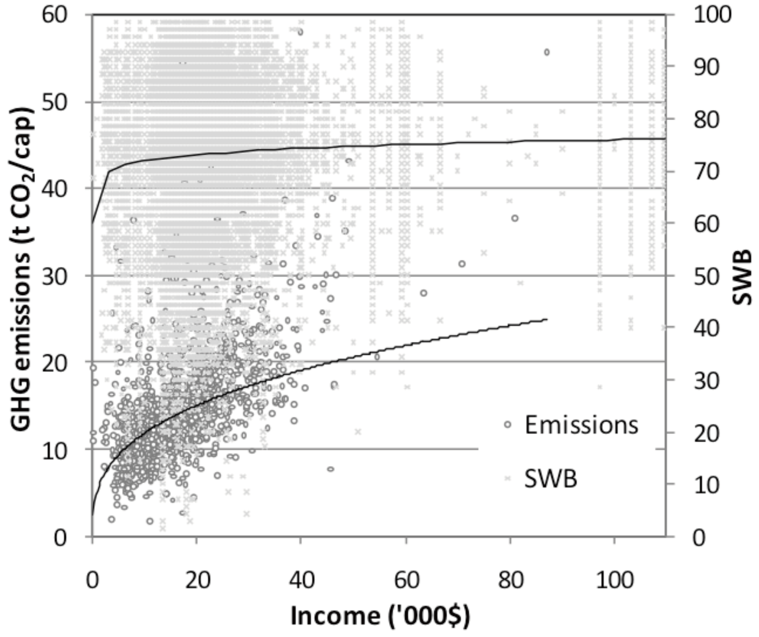
Whilst greenhouse gases can be explained well by the suite of 15 explanatory variables (0.7 ≤ R2 ≤ 0.98, see Appendix D), SWB appears to be also dependent on factors outside our multiple regression, which is why the R2 is low between 0.02 and 0.03 (see the large scatter in Figure 2, left).
-
The regression specifications include a constant term, which is also called a baseline (see Appendix C.1). The baseline explains levels of SWB and GHG emissions that are independent of any of the explanatory variables, whilst effects due to explanatory variables are added to the baseline. The wellbeing baseline is about 50 SWB points. Depending on the regression specification, the per-capita emissions baseline ranges between 0.2 tonnes CO2-e and 1 tonne CO2-e. Our finding is that, while the relationship between income and both SWB and emissions shows diminishing returns, the rate of diminution is faster for SWB, which practically levels off at higher incomes. This result is shown in Figure 2.
As shown in Figure 2, in the stable portion of both relationships above an income of $20,000, a 10% increase in income leads to a 0.4% increase in wellbeing, and in a 2.9% increase in emissions 3. The reasons for these diminishing returns are understood. Taking first emissions, our calculations show that a AU$10,000 increase from a salary of AU$50,000 causes a 6% increase in emissions, but only a 3% increase in emissions from a salary of AU$90,000. This general pattern has been observed by others (for example Wier et al. [51]) and also for other environmental quantities [37]. This can be explained by preferences shifting from emissions-intensive goods to less emissions-intensive services as people move to higher incomes. Diminishing additional wellbeing at increasing incomes has also been almost universally observed [20,52,53,54,55,56,57,58].
Figure 2. Univariate relationship between income and subjective wellbeing (SWB) (upper grey × symbols) and greenhouse gas emissions (GHG) emissions (lower black o symbols).
Challenges 04 00056 g002
Increasing age increases wellbeing by about 0.1 points per additional year of age. A positive effect was also reported by Brereton et al. [57]. Note however that in the raw data, wellbeing decreased from 18–25 years to 45–55 years, and then increases. We are aware that the SWB literature does not usually apply linear forms to model the influence of age. However, given that the importance of age in the regression was rather small, we did not incorporate a quadratic functional form especially to regress the initial decrease. Age has also only a weak effect (+0.1 tonnes CO2-e per year of age) on emissions.
Increasing household size increases wellbeing by about 1.3 points, and decreases per-capita emissions by about 2.4 tonnes CO2-e per additional member. The emissions reductions are largely caused by people sharing household items, as shown previously by Wier et al. [51] and Lenzen et al. [36]. Note however that in the raw data, increasing household size from one adult living alone, to one adult and one child decreases wellbeing.
Increasing population density decreases wellbeing by 0.3 points per 1000 people/km2. Brereton et al. [57] did not find a significant relationship, but this might be due to the difference in regression specifications and variable suites. Since population densities span many orders of magnitude, a logarithmic description is perhaps more appropriate. Here, wellbeing decreases by 0.26 points under a doubling of population density 4. Population density does not have a consistent effect on emissions, although this finding does not agree with results documented elsewhere [36], where except for one sample, emissions decrease with increasing population density. However, the correlations with other HES variables (see Appendix Table C.0) could have a distorting effect. In fact, in the HES sample population density is negatively correlated with expenditures on energy commodities (petrol, natural gas, electricity), which conforms to the notion of urban consolidation reducing energy use. Therefore, the absence of a negative regression coefficient could be caused by the influence of the higher urban incomes. Further, the limitation of the population density variable excludes aspects of varying urban form, and its influence on emissions [60] and wellbeing, through the provision of infrastructure supporting positive work-life balances, social connections, and reducing dependence on energy-intensive transport modes.
Moving up one point on the education qualification scale (see Table A2.2a) increases wellbeing by 0.4 points. A positive effect on wellbeing was also reported by Brereton et al. [57]. Per-capita emissions also increase with qualification, with effects varying around 4 tonnes CO2-e per qualification score. The emissions effect could partly be due to the higher income of more highly qualified people, since there exists some correlation (see Table C.0 in the Appendix).
Moving one point up the tenure (house ownership) scale (see Table A2.3a) increases wellbeing by 2.6 points, hence it appears that this is something Australians find important for wellbeing. Once again, a positive effect was also reported by Brereton et al. [57]. Improving tenure leads to an increase in emissions, but coefficients vary between 1 tonne CO2-e per point.
Adding one car to households’ fleets in the neighbourhood would decrease wellbeing by about 1 point, but would increase emissions by between 3 and 5 tonnes CO2-e. Further robustness tests that excluded Census data resulted in a switch of sign of the emissions regression coefficient (see Appendix D). Hence, while living in areas with high car ownership decreases wellbeing, personal car ownership has the opposite effect.
Moving from the ACT to Victoria, Queensland, South Australia and the Northern Territory is likely to increase wellbeing, but only moving to South Australia and Tasmania would decrease emissions. The latter is due to these States’ high proportion of natural gas and hydropower in the electricity mix, in contrast to the coal-dominated other States, especially the emissions-intensive Victorian brown coal.

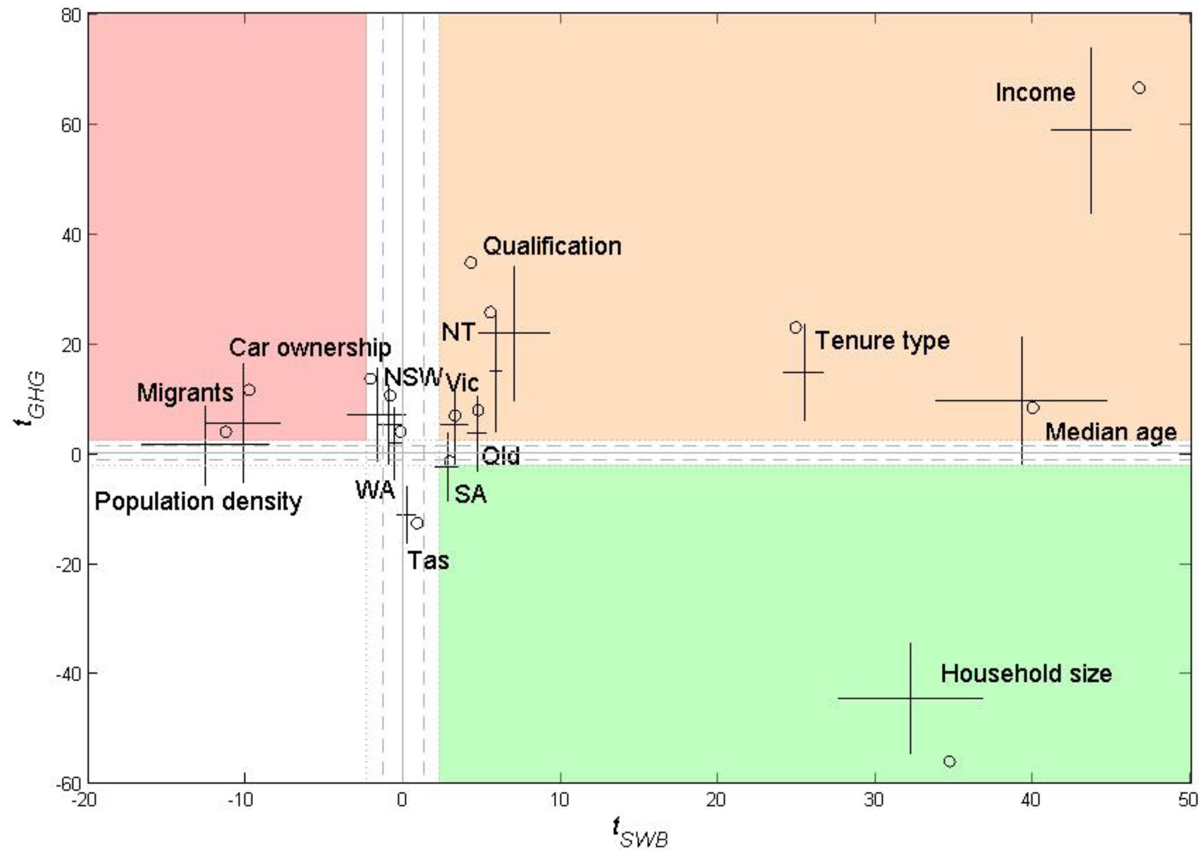
2.4.2. Student’s t Tests

The statistical significance of explanatory variables in explaining a dependent variable is usually measured by applying Student’s t tests. Significance is then expressed as levels of confidence (90%, 95%, or 99%) that regression coefficients for explanatory variables are actually different from zero, and that there is in fact a significant relationship. Figure 3 shows the results of t statistics (no units) across all our regression runs, and plotting their variance as error bars. For example, a positive tGHG for the variable car ownership means that this variable is an “accelerator” of GHG emissions, meaning that an increase in car ownership is positively related to an increase in GHG emissions. Similarly, a negative tSWB for population density means that this variable is a “retardant” for SWB, meaning that an increase in population density is negatively related to subjective wellbeing.
Figure 3. Student’s t statistics for Equations 1d and 3d (o symbols), as well as means and standard deviations (cross-bars) across all regressions. Green: “Win-win” area, orange: “trade-off” area, red: “lose-lose” area. White lines are drawn to delineate areas with t values indicating insufficient significance of regression coefficients.
Challenges 04 00056 g003
The magnitude as well as the relatively small error bars of the t statistics in Figure 3, indicate that many explanatory variables may be significant accelerators or retardants of GHG emissions and SWB. More relevant perhaps, a variable that is a retardant for GHG emissions but an accelerator for SWB would be a candidate for achieving “win-win” policies. Such variables are located in the lower right quadrant of Figure 3 (negative tGHG, and positive tSWB). Similarly, “lose-lose” drivers would be those with positive tGHG and negative tSWB, in the upper left quadrant. The remaining quadrants contain “trade-off” variables, with one beneficial and one adverse influence.
The t statistics indicate the following potential issues of policy relevance in the wellbeing-vs-environment nexus. First, income is associated with a rise in emissions. This result is in accord with numerous previous studies that have demonstrated a link between affluence and emissions 5. However, whilst emissions continue to increase well within the higher income ranges, wellbeing levels off. Hence, increasing gross household income over about $100k on average creates more commons harm than personal good [63].
Second, living together with people is likely to create a win-win situation where both climate and people benefit 6. However, people do not generally choose to live with others who are not their immediate family. Third, increased car ownership will obviously create increased emissions. Personal car ownership enhances subjective wellbeing, but living in an area with high car ownership decreases subjective wellbeing. Fourth, it is interesting that gaining educational qualifications is associated with increased emissions, perhaps through higher income, since qualification and income are correlated.

3. Discussion and Conclusions

Crafting policies that at the same time enhance, or at least not reduce people’s wellbeing, is crucial for the success of government action aimed at mitigation environmental impact. However, there does not yet exist any single contained survey database that allows the unequivocal identification of relationships and trade-offs between wellbeing and the complete environmental impact of households. Those surveys that do contain information pertaining to wellbeing and the environment cover only impacts originating from within the household, but omit the more important indirect effects, or footprints, stemming from the household’s purchasing decisions.
In order to circumvent the lack of comprehensive survey information, we attempt to integrate two separate surveys, and describe the challenges associated with this integration. Subject to our imperfect statistical basis, our results indicate that potential future surveys yielding SWB and carbon footprint simultaneously are likely to come up with carbon footprints increasing with income, but wellbeing levelling off with income. Convincing the public about this detrimental trade-off will likely pose a challenge for policy-making, given its traditional affinity with voter messages predicting increasing wealth. Car ownership is similarly associated with a detrimental trade-off between wellbeing gained through individual transport amenity, but lost through the degradation of the commons. Again, policies will need to strike a wise balance between convenience and wellbeing. In contrast, policies promoting family and other communal living arrangements are likely to succeed in both wellbeing and environmental terms.
The trade-off between qualification and emissions is an interesting one, because it illustrates the well-documented knowledge-concern-action paradox [8,64,65,66,67,68,69,70,71,72]. Whilst people’s knowledge about climate change and personal values appear to cause concern and intent, the latter usually do not translate into personal abatement action and measurable, significant reduction of carbon footprint. Instead, carbon footprint is explained by the socio-economic rather than attitudinal consequences of qualification, as our results indicate. The paradox has been explained by a number of arguments, such as the dominance of convenience and financial constraints over moral imperatives, peer and status pressure, individuals’ lack of agency and trust in authorities, and general lack of abatement opportunities such as public transport [73,74,75]. The lack of consistent individual action may perhaps explain, or may be a result of governments’ reluctance to target consumerism in environmental policies. Some commentators [76,77,78] argue that, in the absence of both public response and technological fixes to the climate change problem [79,80], governments have an obligation to interfere with unsustainable lifestyles.
In focussing on the challenges, necessarily, our work has left open many questions, which is mainly due to the non-existence of a survey that allows deriving SWB and carbon footprint for one and the same population. For example, until a better data foundation exists, there is little reason for (a) further delving into the underlying reasons for some of the broad trends we have identified, and their theoretical underpinnings, (b) drawing conclusions for concrete policy design, and (c) carrying out an in-depth analysis of other environmental indicators such as water use, material flow and land disturbance. Thus, our indicative findings call for an intensified gathering of survey data on both SWB and environmentally relevant information, from one and the same sample population.
Given the imperfect data foundation, it is perhaps premature to discuss in detail possible solutions and recommendations for policy. What is clear however, is that in the long term, intensified surveying can result in the routine establishment of National SWB Accounts [81,82]. Bhutan is leading the world in this respect, and three decades after the Fourth Druk Gyalpo expressed that Gross National Happiness is more important than Gross National Product, Bhutan is now introducing national happiness accounts [83]. SWB is now being more systematically surveyed and reported, for example by the OECD and nef [84,85,86], or in the EC’s Social Survey [87]. Following from the experiences in this work, future national accounts should be completely integrated with respect to information enabling SWB and footprint enumeration. This could take the form envisaged in the UN’s System of Environmental and Economic Accounts (SEEA, [88]), where physical satellite accounts of environmental and resource variables (water, emissions, energy, materials etc.) as well as SWB are spatially disaggregated (to account for urban and rural forms), and arranged as satellites to an input-output system, where the final demand block contains detailed information on household expenditure disaggregated into age, tenure, income and other classes, as already envisaged by [89].
Focusing policy on wellbeing rather than consumption and affluence holds the promise of benefiting the environment, but breaking detrimental addictions with wealth and overcoming detrimental individualism is a daunting societal challenge especially in developed countries where people have experienced convenient suburban lifestyles. Commentators agree that for this to happen a major paradigm shift is necessary [53,63]. Whether such paradigm shifts are likely to be acceptable requires further research such as by Poortinga et al. [90], but even given acceptance, the question remains whether individuals will be capable to carry through the changes that such a shift entails [72].
  • 1. An example is air pollution; References [4,5,6,7] discuss linking data on subjective wellbeing and the environment for the purpose of monetary valuation of environmental quality.
  • 2. Zidanšek also reports a negative correlation between happiness and CO2 emissions intensity (emissions per unit of GDP). However, even though technological progress causes emissions intensities to decrease, total emissions are likely to increase because, in many countries, GDP growth has so far outpaced technological gains [12,13].
  • 3. The linear regression coefficient corresponds to an emissions intensity of 0.4 kg CO2-e/AU$, which is below reported Australian emissions intensities around 0.7 kg CO2-e/AU$ [49]. Similarly, our value of 0.29 for the income-elasticity of emissions is lower than previously measured (0.81, [50]). The reason for these discrepancies is that most previous assessments use univariate instead of multiple regressions, where the method assigned more of the explanatory power to the income variable. Note also that some previous assessments use expenditure as opposed to income as an explanatory variable. The expenditure-elasticity of environmental impact is always higher than its income-elasticity, because some income is not spent at all but saved (see Table 5 in reference [51]).
  • 4. As a reference for readers familiar with Australian geography, such a doubling of population density occurs about each time when progressing from the Pilbara and Kimberleys in WA (0.1 km−2) to Far West NSW (0.2 km−2), then to WA’s Nullarbor Plain (0.4 km−2), to Yorke Peninsula in SA (0.8 km−2), to the Mackay region in Qld (1.6 km−2), to Southern Tasmania (3.8 km−2), to South West WA (6.4 km−2), to the Victorian Gippsland (13.8 km−2), to Barwon outside Melbourne (27 km−2), to the Illawarra south of Sydney (46 km−2), to the Yarra Ranges outside Melbourne (102 km−2), to South East Perth (177 km−2), to Hornsby north of Sydney (407 km−2), to Sydney’s Northern Beaches (860 km−2), to Western Melbourne (1558 km−2), and then to Inner Western Sydney (3201 km−2). In fact, the Grayndler electorate in Sydney’s Inner West scored the lowest level of wellbeing in Australia [59].
  • 5. The overarching link between affluence and emissions has already been taken up by mainstream media [61,62].
  • 6. This finding holds under the assumption of a constant population. That is, if two single-person households merge, then total emissions are likely to decrease. However if a two-person household bears children, the overall emissions are likely to increase. This point was made by an anonymous referee.

Acknowledgments

The authors thank Charles A. J. Vlek, Joy Murray and Charles Berger for valuable comments on earlier drafts of this article. We are also indebted to Ann-Marie James for substantial work on manuscript formatting.

References

  1. Lenzen, M.; Cummins, R.A. Lifestyles and well-being versus the environment. J. Ind. Ecol. 2011, 15, 650–652. [Google Scholar] [CrossRef]
  2. Ferrer-i-Carbonell, A.; Gowdy, J. Environmental degradation and happiness. Ecol. Econ. 2007, 60, 509–516. [Google Scholar] [CrossRef]
  3. Brown, K.W.; Kasser, T. Are psychological and ecological well-being compatible? The role of values, mindfulness, and lifestyle. Soc. Indic. Res. 2005, 74, 349–368. [Google Scholar] [CrossRef]
  4. Welsch, H. Environmental welfare analysis: A life satisfaction approach. Ecol. Econ. 2007, 62, 544–551. [Google Scholar]
  5. Pacione, M. Introduction on urban environmental quality and human wellbeing. Landsc. Urban. Plan. 2003, 65, 1–3. [Google Scholar] [CrossRef]
  6. Smyth, R.; Mishra, V.; Qian, X. The environment and well-being in urban China. Ecol. Econ. 2008, 68, 547–555. [Google Scholar]
  7. MacKerron, G.; Mourato, S. Life satisfaction and air quality in London. Ecol. Econ. 2009, 68, 1441–1453. [Google Scholar] [CrossRef]
  8. Gatersleben, B.; Steg, L.; Vlek, C. Measurement and determinants of environmentally significant consumer behavior. Enviro. Behav. 2002, 34, 335–362. [Google Scholar] [CrossRef]
  9. Veenhoven, R. World Database of Happiness—Correlates of Happiness, 2013. Available online: http://worlddatabaseofhappiness.eur.nl/hap_cor/cor_fp.htm (accessed on 14 April 2013).
  10. Zidanšek, A. Sustainable development and happiness in nations. Energy 2007, 32, 891–897. [Google Scholar] [CrossRef]
  11. nef. Happy Planet Index: 2012 Report—A global index of sustainable well-being, 2012. Available online: http://www.neweconomics.org/publications/happy-planet-index-2012-report (accessed on 14 April 2013).
  12. Wachsmann, U.; Wood, R.; Lenzen, M.; Schaeffer, R. Structural decomposition of energy use in Brazil from 1970 to 1996. Appl. Energy 2009, 86, 578–587. [Google Scholar]
  13. Wood, R. Structural decomposition analysis of Australia’s greenhouse gas emissions. Energy Policy 2009, 37, 4943–4948. [Google Scholar] [CrossRef]
  14. Jackson, T.; Marks, N. Consumption, sustainable welfare and human needs—With reference to UK expenditure patterns between 1954 and 1994. Ecol. Econ. 1999, 28, 421–441. [Google Scholar] [CrossRef]
  15. Jackson, T.; Papathanasopoulou, E. Luxury or “lock-in”? An exploration of unsustainable consumption in the UK: 1968 to 2000. Ecol. Econ. 2008, 68, 80–95. [Google Scholar] [CrossRef]
  16. Druckman, A.; Jackson, T. The carbon footprint of UK households 1990–2004: A socio-economically disaggregated, quasi-multi-regional input–output model. Ecol. Econ. 2009, 68, 2066–2077. [Google Scholar] [CrossRef] [Green Version]
  17. Jackson, T. Prosperity without Growth; Earthscan: London, UK, 2009. [Google Scholar]
  18. Druckman, A.; Jackson, T. The bare necessities: How much household carbon do we really need? Ecol. Econ. 2010, 69, 1794–1804. [Google Scholar] [CrossRef] [Green Version]
  19. Steinberger, J.K.; Krausmann, F.; Eisenmenger, N. Global patterns of materials use: A socioeconomic and geophysical analysis. Ecol. Econ. 2010, 69, 1148–1158. [Google Scholar] [CrossRef]
  20. Steinberger, J.K.; Roberts, J.T. From constraint to sufficiency: The decoupling of energy and carbon from human needs, 1975–2005. Ecol. Econ. 2010, 70, 425–433. [Google Scholar] [CrossRef]
  21. Druckman, A.; Buck, I.; Hayward, B.; Jackson, T. Time, gender and carbon: A study of the carbon implications of British adults’ use of time. Ecol. Econ. 2012, 84, 153–163. [Google Scholar] [CrossRef] [Green Version]
  22. Haberl, H.; Steinberger, J.K.; Plutzar, C.; Erb, K.-H.; Gaube, V.; Gingrich, S.; Krausmann, F. Natural and socioeconomic determinants of the embodied human appropriation of net primary production and its relation to other resource use indicators. Ecol. Indic. 2012, 23, 222–231. [Google Scholar] [CrossRef]
  23. Steinberger, J.K.; Roberts, J.T.; Peters, G.P.; Baiocchi, G. Pathways of human development and carbon emissions embodied in trade. Nat. Clim. Chang. 2012, 2, 81–85. [Google Scholar]
  24. Layard, R. Happiness: Lessons from a New Science; Penguin Press: London, UK, 2005. [Google Scholar]
  25. Kahneman, D.; Krueger, A.B.; Schkade, D.; Schwarz, N.; Stone, A.A. Would you be happier if you were richer? A focusing illusion. Science 2006, 312, 1908. [Google Scholar]
  26. Wiedmann, T.; Minx, J. A Definition of “Carbon Footprint”. Ecological Economics Research Trends; Pertsova, C.C., Ed.; Nova Science Publishers, Inc.: Hauppauge, NY, USA, 2008. Available online: https://www.novapublishers.com/catalog/product_info.php?products_id=5999 (accessed on 18 April 2013).
  27. Lenzen, M. The importance of goods and services consumption in household greenhouse gas emissions calculators. Ambio 2001, 30, 439–442. [Google Scholar]
  28. Cummins, R.A.; Eckersley, R.; Pallant, J.; van Vugt, J.; Misajon, R. Developing a national index of subjective wellbeing: The Australian Unity Wellbeing Index. Soc. Indic. Res. 2003, 64, 159–190. [Google Scholar] [CrossRef]
  29. International Wellbeing Group. Personal Wellbeing Index Manual. Personal Wellbeing Index Manual. 2006. Available online: http://www.deakin.edu.au/research/acqol/instruments/wellbeing-index/ (accessed on 15 April 2013).
  30. Cummins, R.A. Subjective wellbeing, homeostatically protected mood and depression: A synthesis. J. Happiness Stud. 2010, 11, 1–17. [Google Scholar]
  31. Schwarz, N.; Strack, F. Evaluating one’s life: A judgement model of subjective well-being. In Subjective Well-being: An Interdisciplinary Perspective; Strack, F., Argyle, M., Schwarz, N., Eds.; Plenum Press: New York, NY, USA, 1991; pp. 27–47. [Google Scholar]
  32. Schwarz, N. Self-reports: How the questions shape the answers. Am. Psychol. 1999, Feb, 93–105. [Google Scholar] [CrossRef]
  33. Jones, L.V.; Thurstone, L.L. The psychophysics of semantics: An experimental investigation. J. Appl. Psychol. 1955, 39, 31–36. [Google Scholar] [CrossRef]
  34. Cummins, R.A.; Gullone, E. Why we Should Not Use 5-point Likert Scales: The Case for Subjective Quality of Life Measurement. In Proceedings of the Second International Conference on Quality of Life in Cities, National University of Singapore, Singapore, 2000; pp. 74–93.
  35. Herendeen, R.; Tanaka, J. Energy cost of living. Energy 1976, 1, 165–178. [Google Scholar] [CrossRef]
  36. Lenzen, M.; Wier, M.; Cohen, C.; Hayami, H.; Pachauri, S.; Schaeffer, R. A comparative multivariate analysis of household energy requirements in Australia, Brazil, Denmark, India and Japan. Energy 2006, 31, 181–207. [Google Scholar]
  37. Hertwich, E.G. The life-cycle environmental impacts of consumption. Econ. Syst. Res. 2010, 23, 27–47. [Google Scholar] [CrossRef]
  38. Hertwich, E.G. Consumption and industrial ecology. J. Ind. Ecol. 2005, 9, 1–6. [Google Scholar] [CrossRef]
  39. Tukker, A.; Cohen, M.J.; Hubacek, K.; Mont, O. Sustainable consumption and production. J. Ind. Ecol. 2010, 14, 1–3. [Google Scholar] [CrossRef]
  40. ABS, Household Expenditure Survey—Detailed Expenditure Items; ABS Catalogue No. 6535.0; Australian Bureau of Statistics: Canberra, Australia, 2007.
  41. ABS, Australian National Accounts, Input-Output Tables, 2008-09; ABS Catalogue No. 5209.0.55.001; Australian Bureau of Statistics: Canberra, Australia, 2012.
  42. AGO, National Greenhouse Gas Inventory; Department of the Environment and Water Resources, Australian Greenhouse Office: Canberra, Australia, 2009.
  43. ABS, Water Account for Australia 2004-05; ABS Catalogue No. 4610.0; Australian Bureau of Statistics: Canberra, Australia, 2006.
  44. ABS, Integrated Regional Data Base (IRDB); Electronic database, ABS Catalogue No. 1353.0; Australian Bureau of Statistics: Canberra, Australia, 2006.
  45. ABARE. Australian Commodity Statistics, 2009. Available online: http://www.abareconomics.com (accessed on 15 April 2013).
  46. Wood, R.; Lenzen, M.; Foran, B. A material history of Australia: Evolution of material intensity and drivers of change. J. Ind. Ecol. 2009, 13, 847–862. [Google Scholar] [CrossRef]
  47. ISA. Indicators. Information Sheet 6, 2010. Available online: http://www.isa.org.usyd.edu.au/research/InformationSheets/ISATBLInfo6_v1.pdf (accessed on 15 April 2013).
  48. ACQOL. Reports of the Australian Unity Wellbeing Surveys (2001–2010). Available online: http://www.deakin.edu.au/research/acqol/index_wellbeing/index.htm (accessed on 15 April 2013).
  49. Dey, C.; Berger, C.; Foran, B.; Foran, M.; Joske, R.; Lenzen, M.; Wood, R. Household Environmental Pressure from Consumption: An Australian Environmental Atlas. In Water Wind Art and Debate—How Environmental Concerns Impact on Disciplinary Research; Birch, G., Ed.; Sydney University Press: Sydney, Australia, 2007; pp. 280–314. [Google Scholar]
  50. Hertwich, E.G.; Peters, G.P. Carbon footprint of nations: A global, trade-linked analysis. Environ. Sci. Technol. 2009, 43, 6414–6420. [Google Scholar] [CrossRef]
  51. Wier, M.; Lenzen, M.; Munksgaard, J.; Smed, S. Environmental effects of household consumption pattern and lifestyle. Econ. Syst. Res. 2001, 13, 259–274. [Google Scholar] [CrossRef]
  52. Frey, B.S.; Stutzer, A. What can economists learn from happiness research? J. Econ. Lit. 2002, 40, 402–435. [Google Scholar] [CrossRef]
  53. Gowdy, J. Toward a new welfare foundation for sustainability. In Rensselaer Working Papers in Economics Number 0401; Department of Economics, Rensselaer Polytechnic Institute: Troy, NY, USA, 2004. [Google Scholar]
  54. Stutzer, A. The role of income aspirations in individual happiness. J. Econ. Behav. Organ. 2004, 54, 89–109. [Google Scholar] [CrossRef]
  55. Mayraz, G.; Layard, R.; Nickell, S. The functional relationship between income and happiness. In Presented at the 3rd European Conference on Positive Psychology, Braga, Portugal, 3–6 July 2006.
  56. Abdallah, S.; Thompson, S.; Marks, N. Estimating worldwide life satisfaction. Ecol. Econ. 2008, 65, 35–47. [Google Scholar] [CrossRef]
  57. Brereton, F.; Clinch, J.P.; Ferreira, S. Happiness, geography and the environment. Ecol. Econ. 2008, 65, 386–396. [Google Scholar] [CrossRef]
  58. Cummins, R.A.; Collard, J.; Woerner, J.; Weinberg, M.; Lorbergs, W.; Perera, C. Australian Unity Wellbeing index—Report 22.0. The wellbeing of Australians—Who makes the decisions, health/wealth control, financial advice, and handedness. Australian Centre on Quality of Life, School of Psychology, Deakin University: Melbourne, Australia, 2009. Available online: http://www.deakin.edu.au/research/acqol/index_wellbeing/index.htm (accessed on 15 April 2013).
  59. Mead, R.; Cummins, R.A. What Makes Us Happy? Australian Unity and Deakin University: Melbourne, Australia, 2008. [Google Scholar]
  60. Wiedenhofer, D.; Lenzen, M.; Steinberger, J.K. Spatial and socioeconomic drivers of direct and indirect household energy consumption in Australia. In Urban Consumption; Newton, P., Ed.; CSIRO Publishing: Collingwood, VIC, Australia, 2011; pp. 251–266. [Google Scholar]
  61. Monbiot, G. Rich can’t blame the poor for the p-word. Guard Weekly 2008, 24. [Google Scholar]
  62. Monbiot, G. The poor will not destroy the planet. Guard Weekly 2008, 19. [Google Scholar]
  63. Jackson, T. Living better by consuming less? J. Ind. Ecol. 2005, 9, 19–36. [Google Scholar] [CrossRef]
  64. Kempton, W. Will public environmental concern lead to action on global warming? Annu. Rev. Energy 1993, 18, 217–245. [Google Scholar]
  65. Lutzenhiser, L. Social and behavioral aspects of energy use. Annu. Rev. Energy 1993, 18, 247–289. [Google Scholar]
  66. Stokes, D.; Lindsay, A.; Marinopoulos, J.; Treloar, A.; Wescott, G. Household carbon dioxide production in relation to the greenhouse effect. J. Environ. Manage. 1994, 40, 197–211. [Google Scholar] [CrossRef]
  67. McKibben, B. Worried? Us? Granta 2003, 83, 7–12. [Google Scholar]
  68. Poortinga, W.; Steg, L.; Vlek, C. Values, environmental concern, and environmental behaviour. Environ. Behav. 2004, 36, 70–93. [Google Scholar] [CrossRef]
  69. Vringer, K.; Aalbers, T.; Blok, K. Household energy requirement and value patterns. Energy Policy 2007, 35, 553–566. [Google Scholar]
  70. Hertwich, E.G. The environmental effect of car-free housing: A case in Vienna. Ecol. Econ. 2008, 65, 516–530. [Google Scholar] [CrossRef]
  71. Holden, E.; Linnerud, K. Environmental attitudes and household consumption: An ambigous relationship. Int. J. Sustain. Dev. 2010, 13, 217–231. [Google Scholar] [CrossRef]
  72. Whitmarsh, L.; Seyfang, G.; O’Neill, S. Public engagement with carbon and climate change: To what extent is the public “carbon capable”? Glob. Environ. Change 2011, 21, 56–65. [Google Scholar] [CrossRef] [Green Version]
  73. Owens, S. Engaging the public: Information and deliberation in environmental policy. Environ. Plan. A 2000, 32, 1141–1148. [Google Scholar]
  74. Lenzen, M.; Dey, C.J.; Murray, J. A personal approach to teaching about climate change. Austr. J. Environ. Educ. 2002, 18, 35–45. [Google Scholar]
  75. Wilby, P. Grandma’s 80W bulb will kill her grandkids. Guard Weekly 2007, 24. [Google Scholar]
  76. Beekman, V. A green third way? Philosophical reflections on government interventions in non-sustainable lifestyles, 2001. Available online: http://library.wur.nl/WebQuery/wda/lang?dissertatie/nummer=2942PhD (accessed on 15 April 2013).
  77. Beekman, V. Sustainable development and future generations. J. Agric. Environ. Ethics 2004, 17, 3–22. [Google Scholar]
  78. Monbiot, G. Humans cannot be trusted. Guard Weekly 2007, 18. [Google Scholar]
  79. Trainer, F.E. Can renewable energy sources sustain affluent society? Energy Policy 1997, 23, 1009–1026. [Google Scholar]
  80. Trainer, T. Can renewables etc. solve the greenhouse problem? The negative case. Energy Policy 2010, 38, 4107–4114. [Google Scholar] [CrossRef]
  81. Grice, J. National accounts, wellbeing, and the performance of government. Oxf. Rev. Econ. Policy 2011, 27, 620–633. [Google Scholar]
  82. Diener, E.; Tov, W. National Accounts of Well-Being. In Handbook of Social Indicators and Quality of Life Research; Land, K.C., Michalos, A.C., Sirgy, M.J., Eds.; Springer: New York, NY, USA, 2012; pp. 137–158. [Google Scholar]
  83. Government of Bhutan. Bhutan will be the first country with expanded capital accounts. 2012. Available online: http://www.2apr.gov.bt/images/stories/coredoc/remarkbypm.pdf (accessed on 15 April 2013).
  84. OECD. How’s life? Measuring well-being. 2011. Available online: http://www.oecd.org/statistics/howslife.htm (accessed on 15 April 2013).
  85. OECD. Better life initiative: Measuring well-being and progress. OECD: Paris, France, 2012. Available online: http://www.oecd.org/statistics/betterlifeinitiativemeasuringwell-beingandprogress.htm (accessed on 14 April 2013).
  86. nef. National Accounts of Well-being. 2013. Available online: http://www.nationalaccountsofwellbeing.org (accessed on 14 April 2013).
  87. ESS. European Social Survey. 2013. Available online: http://www.europeansocialsurvey.org (accessed on 14 April 2013).
  88. UNSD. Handbook of national accounting: Integrated environmental and economic accounting (SEEA 2003). 2003. Available online: http://unstats.un.org/unsd/envAccounting/seea2003.pdf (accessed on 14 April 2013).
  89. Stone, R. Demographic Input-output: An Extension of Social Accounting; North-Holland Publishing Company: Geneva, Switzerland, 1970. [Google Scholar]
  90. Poortinga, W.; Steg, L.; Vlek, C.; Wiersma, G. Household preferences for energy-saving measures: A conjoint analysis. J. Econ. Psychol. 2003, 24, 49–64. [Google Scholar] [CrossRef]

