Article

Analytic Solution to the Piecewise Linear Interface Construction Problem and Its Application in Curvature Calculation for Volume-of-Fluid Simulation Codes

Biofluid Simulation and Modeling, Theoretische Physik VI, University of Bayreuth, 95448 Bayreuth, Germany
*
Author to whom correspondence should be addressed.
Computation 2022, 10(2), 21; https://doi.org/10.3390/computation10020021
Submission received: 20 November 2021 / Revised: 18 January 2022 / Accepted: 20 January 2022 / Published: 26 January 2022
(This article belongs to the Section Computational Engineering)

Abstract

:
The plane–cube intersection problem has been discussed in the literature since 1984 and iterative solutions to it have been used as part of piecewise linear interface construction (PLIC) in computational fluid dynamics simulation codes ever since. In many cases, PLIC is the bottleneck of these simulations regarding computing time, so a faster analytic solution to the plane–cube intersection would greatly reduce the computing time for such simulations. We derive an analytic solution for all intersection cases and compare it to the previous solution from Scardovelli and Zaleski (Scardovelli, R.; Zaleski, S. Analytical relations connecting linear interfaces and volume fractions in rectangular grids. J. Comput. Phys. 2000, 164, 228–237), which we further improve to include edge cases and micro-optimize to reduce arithmetic operations and branching. We then extend our comparison regarding computing time and accuracy to include two different iterative solutions as well. We find that the best choice depends on the employed hardware platform: on the CPU, Newton–Raphson is fastest with compiler optimization enabled, while analytic solutions perform better than iterative solutions without. On the GPU, the fastest method is our optimized version of the analytic SZ solution. We finally provide details on one of the applications of PLIC—curvature calculation for the Volume-of-Fluid model used for free surface fluid simulations in combination with the lattice Boltzmann method.

1. Introduction

Piecewise linear interface construction (PLIC)—first occurring in the literature for 2D in 1982 [1] and for 3D in 1984 [2]—refers to the problem of calculating the offset along the given normal vector of a plane intersecting a unit cube for a given truncated volume. There are five possible intersection cases (cf. Figure 1), of which the numbers (1), (2) and (5) have been already solved in the original 1984 work by Youngs [2], but the cubic polynomial cases (3) and (4)—considered impossible to algebraically invert [3]—in the majority of the literature are approximated by a Newton–Raphson iterative solution. Nevertheless, there does exist an analytic solution by Scardovelli and Zaleski (SZ) [4] and a single documented implementation thereof in Fortran [5], which also includes an approximative version termed APPLIC.
Here, we formulate the PLIC problem from the ground up—first in the inverse direction—and derive an alternative analytic solution for all intersection cases by inverting the inverse formulation. We then compare our novel solution with (i) the original SZ solution, (ii) an improved and micro-optimized version of the SZ solution developed in the present work, (iii) an iterative solution using Newton–Raphson and (iv) an iterative solution using nested intervals. Depending on the available microarchitecture (GPU/CPU), compiler optimization may strongly favor multiplications and additions while not speeding up trigonometric functions, impacting which of the algorithms is fastest.
Among the applications for PLIC are Volume-of-Fluid simulation codes such as FluidX3D [6,7,8] and others [9,10,11,12,13,14,15,16,17,18,19], often in conjunction with GPU implementations [6,7,8,20,21,22,23,24,25,26] of the lattice Boltzmann method [27,28,29], used for simulating free surface fluid flows. In particular, these simulations work on a cubic lattice, with every lattice point having a fill level assigned to it, and PLIC is used in the process of surface reconstruction during curvature calculation for calculating physical surface tension effects [6,7,8,9]. PLIC-VoF has applications in many areas—for example, computational science [6,7,30,31,32], civil [33,34] and aerospace engineering [35] and computer graphics [36]. In the final section of this work, we provide a detailed overview of the state-of-the-art curvature calculation procedure using PLIC.

2. Plane–Cube Intersection

Inputs to the PLIC algorithm are the truncated volume V 0 [ 0 , 1 ] and the (normalized) normal vector of the plane n = ( n x , n y , n z ) T , | n | = n x 2 + n y 2 + n z 2 = 1 . The desired output is the plane offset from the origin (center of the unit cube) along the normal vector d 0
V 0 , ( n x , n y , n z ) T d 0
where d 0 [ | n x | + | n y | + | n z | 2 , | n x | + | n y | + | n z | 2 ] . The interval is determined by the normal vector orientation: depending on the normal vector, the maximum possible distance from the cube center to be still at least touching the cube in one point varies between 1 2 (normal vector parallel to one of the coordinate system axes) and 3 2 (normal vector along the space diagonal).

2.1. Applying Symmetry Conditions to Reduce Problem Complexity

To reduce the amount of possible cases and to avoid having to consider all possible intersections of the plane and cube edges—following the scheme in [2,15]—the normal vector is component-wise mirrored into positive. (We note that in [15] in Equations (21) and (23), respectively, the “+” should be a “−” and in Equation (24) the “>” should be a “<”.) The mirrored normal vector components are sorted in ascending order according to their magnitude such that 0 n 1 n 2 n 3 1 . Because n is normalized, the absolute value of its largest component n 3 is always greater than zero. In summary, the mirroring removes the sign(s) from n x , n y , n z and and puts them in ascending order, such that normalization still holds: n x 2 + n y 2 + n z 2 = n 1 2 + n 2 2 + n 3 2 = 1 .
n 1 : = min ( | n x | , | n y | , | n z | ) 0
n 3 : = max ( | n x | , | n y | , | n z | ) > 0
n 2 : = | n x | + | n y | + | n z | n 1 n 3 0
Since the function V 0 ( d 0 ) is symmetric around d 0 = 0 and increasing monotonically, the reduced-symmetry-volume V [ 0 , 1 2 ] is limited to the lower half of the intersection volume V 0 and the upper half is reconstructed from symmetry.
V : = 1 2 V 0 1 2
V 0 = sign ( d 0 ) 1 2 V + 1 2
This symmetry condition for the case V 0 > 1 2 is now applied to d 0 , and the coordinate origin is shifted from ( 0 , 0 , 0 ) (center of the unit cube) to ( 1 2 , 1 2 , 1 2 ) (bottom left corner in the back in Figure 1), resulting in the distance d [ 0 , n 1 + n 2 + n 3 2 ] in reduced symmetry space:
d : = n 1 + n 2 + n 3 2 | d 0 |
d 0 = sign V 0 1 2 n 1 + n 2 + n 3 2 d
With this reduction in symmetry, there are only five different intersection cases remaining (see Figure 1).

2.2. Formulating the Inverse PLIC Problem

In order to derive the analytic PLIC solution, first, the inverse problem is formulated in equations—again, following the scheme in [2]. In the inverse problem, the intersection volume is calculated from the plane offset and normal vector as inputs. At first, the intersection points s 1 , s 2 and s 3 of the plane with the coordinate system axes (see Figure 1) are determined:
s 1 : = d n 1 s 2 : = d n 2 s 3 : = d n 3
Now, one calculates the actual volume in reduced symmetry space. The approach is to calculate the volume of the tetrahedral pyramid formed by the plane and the coordinate system axes and, if necessary, subtract the volumes of zero, one, two or all three corners that extend beyond 1. For case (3), an additional condition is required to mutually exclude case (5), in which the bottom four corners of the cube are located beneath the plane.
V = 1 6 s 1 s 2 s 3 if s 1 < 1 1 6 s 2 s 3 s 1 ( s 1 1 ) 1 1 s 1 2 if s 1 1 and s 2 1 1 6 s 3 s 1 s 2 ( s 1 1 ) s 2 1 1 s 1 2 ( s 2 1 ) s 1 1 1 s 2 2 if s 2 1 and s 3 1 and s 1 ( s 2 1 ) s 2 1 6 s 1 s 2 s 3 ( s 1 1 ) s 2 s 3 1 1 s 1 2 ( s 2 1 ) s 1 s 3 1 1 s 2 2 ( s 3 1 ) s 1 s 2 1 1 s 3 2 if s 3 1 1 2 s 3 2 1 s 1 1 s 2 otherwise
To shorten Equation (10), s 1 , s 2 and s 3 are substituted and the expression is simplified, yielding
V = 1 6 n 1 n 2 n 3 · d 3 ( 1 ) if d < n 1 ( d 3 ( d n 1 ) 3 ) ( 2 ) if n 1 d n 2 ( d 3 ( d n 1 ) 3 ( d n 2 ) 3 ) ( 3 ) if n 2 d min ( n 1 + n 2 , n 3 ) ( d 3 ( d n 1 ) 3 ( d n 2 ) 3 ( d n 3 ) 3 ) ( 4 ) if n 3 d 6 n 1 n 2 ( d 1 2 ( n 1 + n 2 ) ) ( 5 ) if min ( n 1 + n 2 , n 3 ) d n 3
which is already considerably more friendly and completes the inverse PLIC formulation in conjunction with Equations (2)–(4), (6) and (7). The condition for case (5) is the remaining free sector of the possible range of d mutually excluded by the other four cases. Listing A1 shows the fully optimized C implementation of the inverse PLIC solution.

2.3. Inverting the Inverse PLIC Formulation Analytically

Equation (11) is now inverted for each case individually. Cases (1), (2) and (5) are easy, but cases (3) and (4) are non-trivial third-order polynomials. Here, we make use of the tool Mathematica, which outputs three complex solutions for cases (3) and (4) each (Appendix A), of which the third solutions, respectively, are the correct ones as their imaginary parts in the desired range are zero after simplification. Luckily, both are of the same overall form (Equation (12)). However, a complex solution is not useful here since the expected result is a real number—a problem known as the casus irreducibilis—and most programming languages cannot deal with complex numbers natively. It would also lead to unwanted computational overhead to carry along the imaginary part during computation, which, in the end, will be zero anyway. To overcome this, we again make use of Mathematica to simplify the general form of the complex solution (Equation (12)) in order to obtain the real, trigonometric solution (Equation (13)):
f ( x , y , a , b , c ) : = c a ( 1 i 3 ) x + i y 3 b ( 1 + i 3 ) x + i y 3
f ( x , y , a , b , c ) : = c 2 a + b x 2 + y 2 3 x 2 + y 2 6 sin π 6 1 3 atan 2 ( y , x )
Equation (13) already is further simplified using the trigonometric identity 3 sin ( α ) cos ( α ) = 2 sin ( π 6 α ) such that the number of trigonometric functions (which are computationally expensive compared to simpler operations such as additions or multiplications) is minimized (Equation (13)).
For better readability, a few expressions are pre-defined. Hereby, the normalization condition n 1 2 + n 2 2 + n 3 2 = 1 is applied.
x 3 : = 81 n 1 n 2 ( n 1 + n 2 2 V n 3 ) > 0
y 3 : = 23328 ( n 1 n 2 ) 3 x 3 2 0
a 3 : = 54 3 n 1 n 2
b 3 : = 1 432 3
c 3 : = n 1 + n 2
t 4 : = 9 ( n 1 + n 2 + n 3 ) 2 18
x 4 : = 324 n 1 n 2 n 3 ( 1 2 V ) 0
y 4 : = 4 t 4 3 x 4 2 0
a 4 : = 1 864 3 t 4
b 4 : = 1 3456 3
c 4 : = n 1 + n 2 + n 3 2
Finally, then, the complete analytic solution to the 3D PLIC problem is given by
d = d 1 = 6 V n 1 n 2 n 3 3 ( 1 ) if d 1 < n 1 d 2 = n 1 2 + 2 V n 2 n 3 1 12 n 1 2 ( 2 ) if n 1 d 2 n 2 d 3 = f ( x 3 , y 3 , a 3 , b 3 , c 3 ) ( 3 ) if n 2 d 3 min ( n 1 + n 2 , n 3 ) d 4 = f ( x 4 , y 4 , a 4 , b 4 , c 4 ) ( 4 ) if n 3 d 4 d 5 = V n 3 + n 1 + n 2 2 ( 5 ) if min ( n 1 + n 2 , n 3 ) d 5 n 3
in conjunction with Equations (2)–(5), (8), (13)–(24).
In Equation (25), it is noteworthy that the conditions for the five different cases are determined a posteriori by the result itself. This means that each case has to be evaluated successively and, for the resulting value d, the respective condition has to be tested. If the condition is true, calculation is stopped and d is returned. If the condition is false, the next case has to be evaluated and so on, until the last case is reached.
The order in which the cases are computed and checked can be optimized to calculate the most difficult and infrequent cases last, when the probability is high that one of the easier and more frequent cases has already been chosen. ‘Frequent’ here refers to some cases appearing more often than others with randomized V 0 and n , as expected in typical PLIC applications. Here, special considerations for edge cases (more on this below) also need to be taken into account to avoid possible divisions by zero. With this in mind, the order ( 5 ) ( 2 ) ( 1 ) ( 3 ) ( 4 ) is preferred.
Additional speedup can be gained by noting that the implicit condition involving d can be replaced by an explicit condition involving V for cases (1), (2) and (5):
d = d 1 = 6 V n 1 n 2 n 3 3 ( 1 ) if 6 V n 2 n 3 < n 1 2 d 2 = n 1 2 + 2 V n 2 n 3 1 12 n 1 2 ( 2 ) if 3 n 2 ( V n 3 + n 1 n 2 ) n 1 2 6 V n 2 n 3 d 3 = f ( x 3 , y 3 , a 3 , b 3 , c 3 ) ( 3 ) if n 2 d 3 min ( n 1 + n 2 , n 3 ) d 4 = f ( x 4 , y 4 , a 4 , b 4 , c 4 ) ( 4 ) if n 3 d 4 d 5 = V n 3 + n 1 + n 2 2 ( 5 ) if n 1 + n 2 2 V n 3
Since V is known, these conditions are checked a priori in order to avoid root function calls if the condition is false.
For even more speedup, all redundant mathematical operations are reduced to a minimum by pre-calculating them to variables (micro-optimization), and condition checks mutually excluded by previous checks are skipped, especially all conditions for the very last case. In the implementation order ( 5 ) ( 2 ) ( 1 ) ( 3 ) ( 4 ) , the conditions for case (3) simplify to d 3 n 3 , which will mutually exclusively decide between cases (3) and (4). Since both d 3 and d 4 are very complicated expressions, here, no simplified a priori condition is formulated.
In Equations (19), (21) and (25), the argument of the square root may be negative before the case condition is tested. In this case—since, in the actual code, floating-point exception handling is turned off for performance reasons—the resulting NaN of a square root of a negative number would not be captured in the case condition, leading to an incorrect result. An additional fdim function call in the square root solves this issue. In the implementation, we artificially exclude the edge case x 4 = 0 in order to, instead of atan 2 ( y , x ) , use the faster atan ( y / x ) , giving the algorithm a 15 % speedup. In case branching would be undesirable, bit masking is also an option, but bit masking turned out to be slower even on GPUs.
Two edge cases still need to be taken into careful consideration: n 1 = 0 (2D) and n 3 = 1 (1D). n 1 = 0 restricts n to be in a 2D plane of two coordinate system axes and n 3 = 1 restricts n to be parallel to one of the coordinate system axes. For the (1D) case, n 3 = 1 and the solution is always (5), so n 1 = n 2 = 0 and min ( n 1 + n 2 , n 3 ) = 0 , simplifying Equation (25) without loss of generality to
d = { V ( 5 ) if 0 d 1
A clean derivation of the 1D case yields
d = V
without any conditions, so it is a necessary requirement that both additional conditions in Equation (27) must be fulfilled automatically. d is in the range 0 d n 1 + n 2 + n 3 2 , so, here, in the special case, we have 0 d 0 + 0 + 1 2 = 1 2 1 , which means that 0 d 1 is indeed fulfilled automatically.
In the (2D) case, n 1 = 0 ( n 2 = 0 is excluded here since it is already covered in the (1D) case, so here n 2 > 0 ). Here, only intersection cases (2) or (5) are possible, 0 < n 2 n 3 1 and min ( n 1 + n 2 , n 3 ) = n 2 , simplifying Equation (25) without loss of generality to
d = 2 V n 2 n 3 ( 2 ) if 0 d n 2 V n 3 + n 2 2 ( 5 ) if n 2 d n 3
A clean derivation of the 2D case yields
d = 2 V n 2 n 3 ( 2 ) if d n 2 V n 3 + n 2 2 ( 5 ) if n 2 d
which has simpler conditions, so again it is a necessary requirement that both additional conditions in Equation (29) must be fulfilled automatically. d is in the range 0 d n 1 + n 2 + n 3 2 , so here, with the special conditions, we have 0 d 0 + n 2 + n 3 2 n 3 + n 3 2 = n 3 , meaning that both 0 d and d n 3 are indeed fulfilled automatically.
In the above chosen ( 5 ) ( 2 ) ( 1 ) ( 3 ) ( 4 ) implementation order, the 1D and 2D special cases are already covered in (5) and (2) at the beginning, so they both are excluded in the remaining intersection cases (1), (3) and (4), meaning that n 1 , n 2 , n 3 > 0 are always given, resulting in x 3 > 0 in Equation (14).
Listing A2 shows the fully optimized C implementation of the analytic PLIC solution with Equation (26).

2.4. The Analytic SZ Solution

The analytic PLIC solution by Scardovelli and Zaleski from 2000 [4] was implemented in Fortran in 2016 by Kawano [5], where it was used as a comparison to the approximative APPLIC method. Here, we focus on the exact SZ solution. The SZ solution is particularly interesting in that it builds upon the L 1 -normalized plane normal vector, instead of the more common L 2 normalization as used in our own solution in Section 2.3. We first translate the Fortran implementation to C, make it compatible with an L 2 -normalized plane normal vector as input and rescale the result from the original [ 0 , 1 ] to [ | n x | + | n y | + | n z | 2 , | n x | + | n y | + | n z | 2 ] . The implementation is provided in Listing A3.
To summarize, the differences between our novel solution and the SZ Kawano implementation are the following:
  • while our solution is based on the L 2 -normalized plane normal vector, the SZ solution uses the L 1 -normalized normal vector;
  • our solution takes two atan operations while the SZ solution takes one acos operation;
  • our solution has a smaller number of arithmetic operations and branching than the SZ Kawano implementation, but requires more special functions.
When closely studying the implementation in Listing A3, we notice that the 1D edge case is poorly handled despite the addition of a tiny constant to the denominator for the calculation of v1. In the edge cases of the normal vector n = ( 1 , 0 , 0 ) T and the volume V 0 { 0 , 1 } , the algorithm returns -NaN both in our OpenCL and in the original Fortran implementation. By checking cases (5) and (2) first and by avoiding divisions by vm1 and vm2 before the checks for cases (5) and (2), respectively, we improve the handling of the 1D edge case. We further apply some micro-optimization to significantly reduce the number of arithmetic operations and branching.
With the knowledge gained from our novel PLIC solution, we are able to make the following improvements to the existing SZ Kawano implementation, resulting in an optimized implementation of the SZ solution as shown in Listing A4:
  • correct edge case behavior;
  • more efficient branching by computing easier, more common cases first and less common, more computationally expensive cases last;
  • micro-optimization by pre-computing redundant terms and minimizing the number of arithmetic operations and branching.

2.5. Iterative Solutions

For comparison, we also provide iterative solutions using nested intervals in Listing A5 and Newton–Raphson in Listing A6.

2.6. Performance and Accuracy Comparison

Apart from floating-point errors, the SZ solution in Listing A4 and our own solution in Listing A2 produce identical results. For accuracy comparison, we define the error as
E i : = | plic _ cube _ inverse ( plic _ cube ( V 0 , n i ) , n i ) V 0 |
with plic _ cube _ inverse ( d 0 , n i ) referring to the implementation in Listing A1 and plic _ cube ( V 0 , n i ) referring to the various PLIC implementations. We define the average error as follows:
E avg : = 1 N L i = 0 N L 1 ( E i )
The execution time for a ‘blank run’
E i , blank : = | plic _ cube _ inverse ( V 0 1 2 , n i ) V 0 |
containing the time for memory loads and stores as well as computing time for the inverse PLIC algorithm is measured and later subtracted from the execution times of the different PLIC variants in order to isolate their execution time. The time is also divided by the number of PLIC function evaluations ( N L ) in order to obtain the time for a single execution.
Table 1 classifies the different PLIC algorithms based on the number and type of operations. Iterative solutions trade special functions (square/cube roots and trigonometric functions) for a larger number of additions and multiplications.

2.6.1. CPU Testing

In this test, n i is set to N = 4096 different normal vectors, of which one is ( 1 , 0 , 0 ) T , one is ( 1 2 , 1 2 , 0 ) T , 510 are random 2D directions in the x-y-plane and the remaining 3584 are random 3D directions. For each of these, the volume V 0 is varied in the interval [ 0 , 1 ] —edge cases included—in L = 4096 equally spaced steps. The test is executed on a single core of a Coffee Lake Intel Core i7-8700K CPU at 4.5 GHz non-AVX2 and 4.0 GHz AVX2 clock frequency with the MSVC C++ compiler. The tests run only on a single CPU core. We cover three scenarios with different compiler flags.
Firstly, we test without any compiler optimization (/Od, /Qpar-). The execution time results are very different, as shown in Table 2. All variants but the Kawano implementation and nested intervals are within the margin of error regarding computing time. In the edge cases of the normal vector n = ( 1 , 0 , 0 ) T and the volume V 0 { 0 , 1 } , the SZ solution by Kawano returns -NaN, which propagates through the entire error averaging procedure. For the IEEE-754 FP32 floating-point format, the machine epsilon is at ϵ = 5.96 × 10 8 , meaning that, for all other PLIC variants, the average error E avg is within machine precision.
Secondly, we repeat the test with compiler optimizations enabled, but with AVX2 disabled. The used compiler flags are /O2, /Oi, /Ot, /Qpar- and /fp:except-. The results are presented in Table 3. Here, Newton–Raphson considerably outperforms all the other solutions.
Lastly, we test with full compiler optimizations and AVX2. The used compiler flags are /O2, /Oi, /Ot, /Qpar, /arch:AVX2 and /fp:except-. The results are presented in Table 4. In all variants, execution times do not significantly differ from when AVX is disabled, indicating that auto-vectorization is not being applied at all. As an additional indicator, the CPU clock frequency does not drop by the AVX2 clock offset while the tests are running.

2.6.2. GPU Testing

Since, in many applications, the target platform for the PLIC algorithm is the GPU, we also benchmark the different variants in OpenCL on an Nvidia Titan Xp GPU (3840 CUDA cores at 1582 MHz , 12.1 TFLOPs / s , driver version 442.59 , OpenCL 1.2 ). The test here differs from the CPU C++ test in that, for sufficient saturation of the parallel computing capabilities, the number of random normal vectors is increased to 67,108,864, of which again one is ( 1 , 0 , 0 ) T , one is ( 1 2 , 1 2 , 0 ) T , 8,388,606 are random 2D directions in the x-y-plane and the remaining 58,720,256 are random 3D directions. For these normal vectors, PLIC is run in parallel and, for each of them, the volume V 0 is varied in the interval [ 0 , 1 ] —edge cases included—in L = 256 equally spaced steps in series. For more accurate results through averaging, this test is run 64 times and the mean execution time is averaged and divided by the number of parallel and serial PLIC computations, resulting in an average computing time that is more than three magnitudes shorter than for single-core CPU execution, as listed in Table 5. Even though the tests are designed differently for the CPU and GPU, this comparison is appropriate because, in both cases, the same algorithms are computed and the hardware is fully saturated. The table also includes the number of arithmetic operations (floating-point, integer and bit operations combined) N a and the number of branching operations N b in PTX assembly [37]. GPUs are especially poor at branching, so a small N b is desired. These operation counts—in analogy to the computing time—refer to the isolated PLIC variants with the background ‘blank run’ for memory loads and stores as well as the inverse PLIC algorithm subtracted. N a indicates that Newton–Raphson is unrolled by the compiler, whereas nested intervals are not. The number of iterations to reach machine precision for nested intervals depends on the initial interval width, which is a function of the normal vector components. For Newton–Raphson, the number of branching operations N b is the smallest, resulting in rather good performance. Nevertheless, our optimized implementation of the SZ solution pulls ahead rather significantly and thus is preferred by us.
By dividing N a by the execution time, we obtain the performance in TFLOPs/s (integer and bit operations are included since these are performed on the same CUDA cores as floating-point operations on Nvidia Pascal), showing that computing efficiency is not significantly impacted by the special functions used in the analytic solutions.
It is noteworthy that there also is a novel neural network-based approach termed NPLIC that promises significant speedup, especially for more complex, non-cubic lattices [38]. This approach efficiently works on GPU hardware by using mainly multiplication and addition.

3. Application: Curvature Calculation for VoF-LBM on the GPU

3.1. Volume-of-Fluid Overview

Volume-of-Fluid (VoF) is a model to simulate a sharp, freely moving interface between a fluid and gas phase in a Cartesian lattice [9,10,11,12]. While it can be coupled to any flow solver, here, we focus on its usage in conjunction with the lattice Boltzmann method (LBM). The interface is ensured to be exactly one lattice cell thick at any time (illustrated in Figure 2). As an indicator for each lattice point type, the fill level φ is introduced, whereby, for fluid lattice points φ = 1 , for interface 1 > φ > 0 and for gas φ = 0 :
φ ( x , t ) : = m ( x , t ) ρ ( x , t ) = 1 if x is f l u i d ] 0 , 1 [ if x is i n t e r f a c e = 0 if x is g a s
Here, ρ is the density provided by the lattice Boltzmann method (LBM) and m is the fluid mass. m is a conserved quantity and cannot be gained or lost, only moved within the simulation box. Isolated interface cells are not allowed to exist. If an interface cell has no fluid neighbors, it is converted to gas. Its remaining mass is distributed as excess mass to neighboring interface cells. The details are described in [8].
The key difficulty of modeling a free surface on a discretized lattice is to obtain the surface curvature, which is a necessary ingredient for calculating the surface tension via the Young–Laplace pressure
Δ p = 2 σ κ
with κ = 1 R denoting the local mean curvature and σ denoting the surface tension parameter of the simulated fluid. The equation is easy in principle, but calculating κ from the discretized interface geometry is not. Specifically, discretized interface here means that only a local 3 3 neighborhood of fill levels φ [ 0 , 1 ] is known, in addition to the point in the center of this neighborhood being an interface lattice point.
φ 0 , , φ 26 κ
The most common algorithm in the literature [9,12] is the curvature calculation via a least-squares paraboloid fit from a neighborhood of points located on the interface. It assumes the local interface to be a paraboloid, the specifics of which will be given in the following sections. Finding an appropriate set of neighboring points on the interface requires the PLIC solution.

3.2. Obtaining Neighboring Interface Points: PLIC Point Neighborhood

Piecewise linear interface construction works on a 3 3 neighborhood of an interface lattice point (illustrated in 2D in Figure 3a). Within this neighborhood, only interface points other than the center interface point—which is always interface—are considered as candidates for the later fitting procedure (Figure 3b). The difficult part is to accurately obtain the heights z i of at least five neighboring points located on the true interface (Figure 3c). For this, first, the normal vector n of the center interface point is calculated via the Parker–Youngs approximation as described in the Appendix C.1 in Equation (A4). A new coordinate system is introduced, with its first base vector b z defined as this normal vector. Then, the cross product with an arbitrary vector such as
r : = ( 0.56270900 , 0.32704452 , 0.75921047 ) T
which is always non-colinear with b z by random chance is calculated to provide second and third orthonormal vectors
b z : = n
b y : = b z × r | b z × r |
b x : = b y × b z
forming the new coordinate system in which the z-axis is colinear with the surface normal and the center interface point is in the origin. Now, the relative positions e i of all neighboring interface lattice points (equal to the D3Q27 LBM streaming directions, Equation (A2)) are gathered and transformed into the rotated coordinate system. During this step, the approximate interface position of neighboring interface points (streaming directions, Figure 3b) is corrected to the much more accurate interface position via the PLIC plane–cube intersection solution (Section 2, Figure 3c,d):
p i = x i y i z i : = e i · b x e i · b y e i · b z + d 0 ( φ i , n ) d 0 ( φ 0 , n )
Here, i is only the subset of { 0 , , 26 } for which 0 < φ i < 1 is true (interface points). d 0 ( V 0 = φ i , n ) denotes the PLIC function (Equation (8)). Note that d 0 ( V 0 = φ 0 , n ) only needs to be calculated once, while d 0 ( V 0 = φ i , n ) has to be calculated for each neighboring interface point, and that the normal vectors of neighboring interface lattice points are approximated to be equal to the normal vector of the center lattice point. In theory, going with the separately calculated neighbor normal vectors—which would require either an additional data buffer for normal vectors in memory or alternatively a 5 3 neighborhood, which would break the multi-GPU capabilities of the code—should be more accurate, but our practical tests indicated no significant difference (see Figure 4).
The set of points p i is then used to fit a local paraboloid. This paraboloid (Figure 3e) here lacks a vertical offset parameter as that is handled already by the center point being defined as the origin, reducing the computational cost to an LU decomposition of dimensionality N = 5 . The paraboloid has the form
z ( x , y ) = A x 2 + B y 2 + C x y + H x + I y = : x · Q
with
x : = ( A , B , C , H , I ) T
Q : = ( x 2 , y 2 , x y , x , y ) T
The solution vector x and thus the fitting parameters are calculated following the procedure in Appendix C.3. Finally, the constants A, B, C, H and I are inserted into the analytic equation for the curvature (A13), completing the algorithm.

3.3. Validating Curvature Calculation

To test the accuracy of the presented curvature calculation method, we validate it on spherical drops of different radius R = 1 κ theo . The fill levels φ are initialized with the inverse PLIC algorithm. To let the drop relax and the error converge, we simulate up to 50,000 LBM time steps with D3Q19 SRT ( τ = 1 , σ = 0.001 ). The curvature error is calculated using the L 1 error norm with summation over all interface points:
E ( κ ) : = | κ sim κ theo | κ theo
We plot the error in Figure 4. For low drop radius R 32 , the error of our proposed method (red curve) is around 0.5 % and the local distribution of the error on the sphere is very homogeneous (Figure 5). As R is increased, the error also generally increases and points with particularly large errors emerge on the sphere surface. This can be assuming that κ sim is accurate to some statistically distributed error ϵ , κ sim = κ theo ± ϵ . When ϵ remains independent of R, the relative error | κ sim κ theo | κ theo = ϵ R will increase proportionally with R. The curvature-independent error ϵ in turn arises from the so-called staircase effect, in which the numerical curvature of a flat plane is non-zero if the plane is not aligned with one of the coordinate axes. In Figure 6, we demonstrate this effect quantitatively.
If we do not make the assumption that the PLIC normal direction of neighbor interface points has to equal the center normal vector (orange curve), then accuracy is slightly improved. However, the additional computational complexity may not justify this small improvement in accuracy.
For comparison, we also plot the curvature approximation method proposed by Donath [17] without and with the proposed π 4 correction factor. As expected, the error is much larger, but this method is also computationally less expensive than ours and certainly has its use-cases as well.

3.4. Application Example: Simulating a Terminal Velocity Raindrop Impact

The analytic plane–cube intersection solution presented in this work has originally been developed for the VoF-LBM GPU simulation code FluidX3D, where we could observe a significant speedup compared to when an iterative nested-intervals solution is used. To illustrate this particular application of PLIC, we show a simulation of a 5 mm diameter raindrop impact at terminal velocity in Figure 7. The parameters for this simulation are ν = 1.307 × 10 6 m 2 s , ρ = 999.7 kg m 3 , σ = 74.2 × 10 3 kg s 2 , g = 9.81 m s 2 , d = 0.005 m , u = 9.2 m s , resulting in the dimensionless numbers Re = 35195 , We = 5702 , Fr = 41.54 , Ca = 0.1620 , Bo = 3.3042 . The simulation box has the dimensions 5.00 cm × 5.00 cm × 4.25 cm and the pool height is 2.00 cm . The simulation code FluidX3D is documented in great detail in [8]. A large-scale computational study on these raindrop impact simulations was conducted in [6], alongside extensive validation of the method, showing very good agreement with experiments. At this large Reynolds number, there is only a small gap of possible LBM unit parametrization to have stable simulations and only the SRT collision operator remains stable; details can be found in SI Section S3 in [6].
The t = 0.005 s of computed time is equivalent to 4907 LBM time steps at 400 × 400 × 340 lattice resolution. Computing time with a Nvidia Titan Xp GPU is 59.7 s with our optimized version of the SZ solution (Listing A4). When removing PLIC from the LBM algorithm, computing time is 51.2 s , meaning that 14.3 % of the entire computing time is spent on the PLIC routine. This fraction of course depends on the simulation itself and the amount of surface area where curvature is computed, but it should give an impression of the significance of an efficient PLIC implementation for computing time. For comparison, with nested intervals (Listing A5), the total computing time for the raindrop increases to 68.0 s , so this PLIC routine would take 32.8 % of the total computing time.

4. Conclusions

We derived an analytic solution to the PLIC problem and compared it to the existing solution by Scardovelli and Zaleski [4] in two variants: an implementation by Kawano [5] and an improved and micro-optimized version thereof. We furthermore compared these three analytic solutions to two iterative solutions using Newton–Raphson and nested intervals. We provide C implementations of all variants as well as the inverse PLIC formulation.
We observe that, in a benchmark scenario with compiler optimization on the CPU, the Newton–Raphson solution (Listing A6) is considerably faster than all other solutions. Without compiler optimization, execution times for our novel solution and our optimized version of the SZ solution are both faster than Newton–Raphson.
On the GPU, the analytic solutions are faster than the iterative solutions, with our micro-optimized version of the SZ solution as presented in Listing A4 being fastest. For a generic PLIC problem, this is the solution we recommend.
In the most common application of PLIC—curvature calculation for Volume-of-Fluid LBM, which we presented and also validated on spherical drops—profiling revealed PLIC to be the main bottleneck regarding computing time. Here, our proposed fast PLIC solution led to significant speedup of VoF calculations. We hope that our findings will also make other simulation codes more computationally efficient.

Author Contributions

Analytic calculations were performed by M.L. M.L. conducted programming and testing. M.L. wrote the initial draft and created the illustrations. M.L. and S.G. performed review and editing on the draft. All authors have read and agreed to the published version of the manuscript.

Funding

This study was funded by the Deutsche Forschungsgemeinschaft (DFG, German Research Foundation)—Project Number 391977956—SFB 1357, and Number 491183248. Funded by the Open Access Publishing Fund of the University of Bayreuth.

Data Availability Statement

All data are archived and available upon request. All code beyond what is provided in the listings is archived and available upon request.

Acknowledgments

We acknowledge funding and support from the SFB 1357 Mikroplastik. We gratefully acknowledge the computing time provided by the SuperMUC system of the Leibniz Rechenzentrum, Garching. We further acknowledge support through the computational resources provided by the Bavarian Polymer Institute. We acknowledge the NVIDIA Corporation for donating a Titan Xp GPU for our research. M.L. acknowledges support from the ENB Biological Physics.

Conflicts of Interest

The authors declare no potential conflicts of interests.

Abbreviations

The following abbreviations are used in this manuscript:
AVX2advanced vector extensions 2 (256-bit)
CPUcentral processing unit
GPUgraphics processing unit
LBMlattice Boltzmann method
PLICpiecewise linear interface construction
VoFVolume-of-Fluid

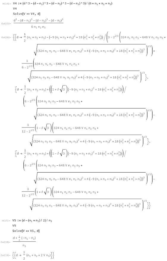
Appendix A. PLIC Inversion with Mathematica

Computation 10 00021 i001Computation 10 00021 i002Computation 10 00021 i003

Appendix B. Code Listings

Listing A1. Fully optimized C implementation of the inverse PLIC solution. To avoid branching between cases (3) and (4), in the implementation, the fdimf(x,y):= max(x-y,0) function is used. Case (2) cannot be included with another fdimf(x,y) because, in case (2), division by n1 must be avoided since it could be zero.
float plic_cube_inverse(const float d0, const float nx, const float ny, const float nz) { // unit cube - plane intersection
      ↪: plane offset d0, normal vector n -> volume V0 in [0,1]
 const float n1 = fmin(fmin(fabs(nx), fabs(ny)), fabs(nz)); // eliminate most cases due to symmetry
 const float n3 = fmax(fmax(fabs(nx), fabs(ny)), fabs(nz));
 const float n2 = fabs(nx)-n1+fabs(ny)+fabs(nz)-n3;
 const float d = 0.5f*(n1+n2+n3)-fabs(d0); // calculate PLIC with reduced symmetry, shift origin from (0.0,0.0,0.0) ->
       ↪ (0.5,0.5,0.5)
 float V;  // 0.0<=V<=0.5
 if(fmin(n1+n2, n3)<=d && d<=n3) {  // case (5)
  V = (d-0.5f*(n1+n2))/n3; // avoid division by n1 and n2
 } else if(d<n1) {  // case (1)
  V = cb(d)/(6.0f*n1*n2*n3);  // condition d<n1==0 is impossible if d==0.0f
 } else if(d<=n2) { // case (2)
  V = (3.0f*d*(d-n1)+sq(n1))/(6.0f*n2*n3);  // avoid ;division by n1
 } else {  // case (3) or (4)
  V =  (cb(d)-cb(d-n1)-cb(d-n2)-cb(fdim(d, n3)))/(6.0f*n1*n2*n3);
 return copysign(0.5f-V, d0)+0.5f;  // apply symmetry for V0>0.5
}
Listing A2. Fully optimized C implementation of our analytic PLIC solution.
float plic_cube_reduced(const float V, const float n1, const float n2, const float n3) {
 const float n1pn2=n1+n2, n3xV=n3*V;
 if (n1pn2<=2.0f*n3xV) return n3xV+0.5f*n1pn2; // case (5)
 const float V6n2n3=6.0f*n2*n3xV, sqn1=sq(n1);
 if (V6n2n3>=sq(n1) && 3.0f*n2*(2.0f*n3xV+n1-n2)<=sqn1) return ;0.5f*n1+0.28867513f*sqrt(24.0f*n2*n3xV-sqn1); // case (2)
 if (V6n2n3<sqn1) return cbrt(V6n2n3*n1); // case (1)
 const float n1xn2=n1*n2;
 const float x3 = 81.0f*n1xn2*(n1pn2-2.0f*n3xV); // x3>0
 const float y32 = fdim(23328.0f*cb(n1xn2), sq(x3)); // y3>=0
 const float u3 = cbrt(sq(x3)+y32);
 const float d3 = n1pn2-(7.5595264f*n1xn2+0.26456684f*u3)*rsqrt(u3)*sin(0.5235988f-0.33333334f*atan(sqrt(y32)/x3)); // x3
       ↪ >0
 if(d3<=n3) return d3; // case (3)
 const float t4 = 9.0f*sq(n1pn2+n3)-18.0f;
 const float x4 =  fmax(n1xn2*n3*(324.0f-648.0f*V), 1.1754944E-38f); // avoid edge  case V==0.5 to make x4>0
 const float y42 = 4.0f*cb(t4)-sq(x4); //  y4>=0
 const float u4 = cbrt(sq(x4)+y42);
 const float d4 = 0.5f*(n1pn2+n3)-(0.20998684f*t4+0.13228342f*u4)*rsqrt(u4)*sin(0.5235988f-0.33333334f*atan(sqrt(y42)/x4))
       ↪ // x4>0
 return d4; // case (4)
}
float  plic_cube(const float V0, const float nx, const float ny, const float nz) {  // unit cube - plane intersection: volume
      ↪ V0 in [0,1], normal vector n -> plane offset d0
 const float ax=fabs(nx), ay=fabs(ny), az=fabs(nz), V=0.5f-fabs(V0-0.5f); // eliminate symmetry cases
 const float n1 = fmin(fmin(ax, ay), az);
 const float n3 = fmax(fmax(ax, ay),  az);
 const float n2 = ax-n1+ay+az-n3;
 const float d = plic_cube_reduced(V, n1, n2, n3); //  calculate PLIC with reduced symmetry
 return copysign(0.5f*(n1+n2+n3)-d, V0-0.5f);  // apply  symmetry for V0>0.5
}
Listing A3. The Fortran implementation [5] of the analytic SZ PLIC solution [4] translated to C without further optimization.
float plic_cube(const float V0, const float nx, const float ny, const float nz) { // unit cube - plane intersection: volume
      ↪ V0 in [0,1], normal vector n -> plane offset d0
 const float l = fabs(nx)+fabs(ny)+fabs(nz); // length in L1 norm
 const float ax=fabs(nx)/l, ay=fabs(ny)/l, az=fabs(nz)/l, w=0.5f-fabs(V0-0.5f); // eliminate symmetry cases
 const float vm1 = fmin(fmin(ax, ay), az);
 const float vm3 = fmax(fmax(ax, ay), az);
 const float vm2 = fdim(1.0f, vm1+vm3); // ensure vm2>=0
 const float vm12 = vm1+vm2;
 float alpha = 0.0f;
 const float v1 = sq(vm1)/(6.0f*vm2*vm3+1E-25f);
 const float w6 = 6.0f*vm1*vm2*vm3*w;
 if(w<v1) {
  alpha = cbrt(w6); // case (1)
 } else if(w<v1+0.5f*(vm2-vm1)/vm3) {
  alpha = 0.5f*(vm1+sqrt(sq(vm1)+8.0f*vm2*vm3*(w-v1))); // case (2)
 } else {
  float v3;
  if(vm3<vm12) {
   v3 =  (sq(vm3)*(3.0f*vm12-vm3)+sq(vm1)*(vm1-3.0f*vm3)+sq(vm2)*(vm2-3.0f*vm3))/(6.0f*vm1*vm2*vm3);
  } else {
   v3 = 0.5f*vm12/vm3;
   if(v3<=w) alpha = vm3*w+0.5f*vm12; // case (5)
  }
  if(alpha==0.0f) {
   float a0, a1, a2;
   if(w<v3) { // case (3)
    a2 = -3.0f*vm12;
    a1 = 3.0f*(sq(vm1)+sq(vm2));
    a0 = w6-cb(vm1)-cb(vm2);
   } else { // case (4)
    a2 = -1.5f;
    a1 = 1.5f*(sq(vm1)+sq(vm2)+sq(vm3));
    a0 = 0.5f*(w6-cb(vm1)-cb(vm2)-cb(vm3));
   }
   const float q0 =  0.16666667f*(a1*a2-3.0f*a0)-3.7037037E-2f*cb(a2); // 3.7037037E-2f = 1/27
   const float sp = sqrt(0.11111111f*sq(a2)-0.33333334f*a1);
   alpha = 2.0f*sp*cos(4.1887902f+0.33333334f*acos(q0/cb(sp)))-0.33333334f*a2; // 4.1887902f = 4/3*pi
  }
 }
return l*copysign(0.5f-alpha, V0-0.5f); // rescale result  and apply symmetry for V0 0.5
}
Listing A4. Fully optimized C implementation of the SZ PLIC solution.
float plic_cube_reduced(const float V, const float n1, const float n2, const float n3) { // optimized solution from SZ and
      ↪ Kawano
 const float n12=n1+n2, n3V=n3*V;
 if(n12<=2.0f*n3V) return n3V+0.5f*n12; // case (5)
 const float sqn1=sq(n1), n26=6.0f*n2, v1=sqn1/n26; // after case (5) check n2>0 is true
 if(v1<=n3V && n3V<v1+0.5f*(n2-n1))  return  0.5f*(n1+sqrt(sqn1+8.0f*n2*(n3V-v1))); // case (2)
 const float V6 = n1*n26*n3V;
 if(n3V<v1) return cbrt(V6); // case (1)
 const float v3 = n3<n12 ? (sq(n3)*(3.0f*n12-n3)+sqn1*(n1-3.0f*n3)+sq(n2)*(n2-3.0f*n3))/(n1*n26) : 0.5f*n12; // after case
       ↪ (2) check n1>0 is true
 const float sqn12=sqn1+sq(n2), V6cbn12=V6-cb(n1)-cb(n2);
 const bool case34 = n3V<v3;  // true: case (3), false: case (4)
 const float a = case34 ? V6cbn12  : 0.5f*(V6cbn12-cb(n3));
 const float b = case34 ? sqn12 : 0.5f*(sqn12+sq(n3));
 const float c = case34 ? n12 : 0.5f;
 const float t = sqrt(sq(c)-b);
 return  c-2.0f*t*sin(0.33333334f*asin((cb(c)-0.5f*a-1.5f*b*c)/cb(t)));
}
float plic_cube(const float V0, const float nx, const float ny, const float nz) { // unit cube - plane intersection: volume
      ↪ V0 in [0,1], normal vector n -> plane offset d0
 const float ax=fabs(nx), ay=fabs(ny), az=fabs(nz), V=0.5f-fabs(V0-0.5f), l=ax+ay+az; // eliminate symmetry cases,
       ↪ normalize n using L1 norm
 const float n1 = fmin(fmin(ax, ay), az)/l;
 const float n3 = fmax(fmax(ax, ay), az)/l;
 const float n2 = fdim(1.0f, n1+n3); // ensure n2>=0
 const float d = plic_cube_reduced(V, n1, n2, n3); // calculate PLIC with reduced symmetry
 return l*copysign(0.5f-d, V0-0.5f); // rescale result and apply symmetry for V0>0.5
}
Listing A5. C implementation of the iterative nested-intervals solution for cases (3) and (4).
int log2_fast(const float x) { // evil log2 hack: log2(x)=(as_uint(x)>>23)-127
 return (as_uint(x)>>23)-127;
}
float plic_cube_reduced(const float V, const float n1, const float n2, const float n3) {
 const float n1pn2=n1+n2, n3xV=n3*V;
 if(n1pn2<=2.0f*n3xV) return n3xV+0.5f*n1pn2; // case (5)
 const float V6n2n3=6.0f*n2*n3xV, sqn1=sq(n1);
 if(V6n2n3>=sq(n1) && 3.0f*n2*(2.0f*n3xV+n1-n2)<=sqn1) return 0.5f*n1+0.28867513f*sqrt(24.0f*n2*n3xV-sqn1); // case (2)
 if(V6n2n3<sqn1) return cbrt(V6n2n3*n1); // case (1)
 const float V6n1n2n3 = V6n2n3*n1;
 float dmin, dmax, d;
 uint k;
 dmin=n2; dmax=n1+n2; d=0.5f*(dmin+dmax);
 k = (uint)log2_fast((dmax-dmin)*1.67772162E7f); // deterdmine number of interval halvings to reach machine precision
 for(uint i=0; i<=k; i++) {
  if(cb(d)-cb(d-n1)-cb(d-n2)<V6n1n2n3) dmin = d;
  else dmax = d;
  d = 0.5f*(dmin+dmax);
}
 if(d<=n3) return d; // case (3)
 dmin=n3; dmax=0.5f*(n1+n2+n3); d=0.5f*(dmin+dmax);
 k = (uint)log2_fast((dmax-dmin)*1.67772162E7f); // deterdmine number of interval halvings to reach machine precision
 for(uint i=0; i<=k; i++) {
  if(cb(d)-cb(d-n1)-cb(d-n2)-cb(d-n3)<V6n1n2n3) dmin = d;
  else dmax = d;
  d = 0.5f*(dmin+dmax);
}
 return d;
}
float plic_cube(const float V0, const float nx, const float ny, const float nz) {
 const float n1 = fmin(fmin(fabs(nx), fabs(ny)), fabs(nz)); // eliminate most cases due to symmetry
 const float n3 = fmax(fmax(fabs(nx), fabs(ny)), fabs(nz));
 const float n2 = fabs(nx)-n1+fabs(ny)+fabs(nz)-n3;
 const float V = 0.5f-fabs(V0-0.5f);
 const float d = plic_cube_reduced(V, n1, n2, n3);
 return copysign(0.5f*(n1+n2+n3)-d, V0-0.5f);  // apply symmetry for V0>0.5
}
Listing A6. C implementation of the iterative Newton–Raphson solution for cases (1), (3) and (4). Calculating case (1) with Newton–Raphson as well instead of the cbrt() function results in a very small but noticeable improvement in performance when executed on the CPU.
float plic_cube_reduced(const float V, const float n1, const float n2, const float n3) {
 const float n1pn2=n1+n2, n3xV=n3*V;
 if(n1pn2<=2.0f*n3xV) return n3xV+0.5f*n1pn2; // case (5)
 const float V6n2n3=6.0f*n2*n3xV, sqn1=sq(n1);
 if(V6n2n3>=sq(n1) && 3.0f*n2*(2.0f*n3xV+n1-n2)<=sqn1) return  0.5f*n1+0.28867513f*sqrt(24.0f*n2*n3xV-sqn1); // case (2)
 const float V6n1n2n3 = V6n2n3*n1;
 float dmin, dmax, d;
 if(V6n2n3<sqn1) {
  dmin=0.0f; dmax=n1; d=0.5f*(dmin+dmax);
  for(uint i=0; i<7; i++) {
   const float f = cb(d)-V6n1n2n3;
   const float fs = 3.0f*sq(d);
   d -= f/fs;
  }
  return d; // case (1)
} 
 dmin=n2; dmax=n1+n2; d=0.5f*(dmin+dmax);
 for(uint i=0; i<4; i++) {
  const float f = cb(d)-cb(d-n1)-cb(d-n2)-V6n1n2n3;
  const float fs = 3.0f*(sq(d)-sq(d-n1)-sq(d-n2));
  d -= f/fs;
}
 if(d<=n3) return d; // case (3)
 dmin=n3; dmax=0.5f*(n1+n2+n3); d=0.5f*(dmin+dmax);
 for(uint i=0; i<4; i++) {
  const float f = cb(d)-cb(d-n1)-cb(d-n2)-cb(d-n3)-V6n1n2n3;
  const float fs = 3.0f*(sq(d)-sq(d-n1)-sq(d-n2)-sq(d-n3));
  d -= f/fs;
}
 return d; // case (4)
}
float plic_cube(const float V0, const float nx, const float ny, const float nz) {
 const float n1 = fmin(fmin(fabs(nx), fabs(ny)), fabs(nz)); // eliminate most cases due to symmetry
 const float n3 = fmax(fmax(fabs(nx), fabs(ny)), fabs(nz));
 const float n2 = fabs(nx)-n1+fabs(ny)+fabs(nz)-n3;
 const float V = 0.5f-fabs(V0-0.5f);
 const float d = plic_cube_reduced(V, n1, n2, n3);
 return copysign(0.5f*(n1+n2+n3)-d, V0-0.5f); // apply symmetry for V0>0.5
}

Appendix C. Paraboloid Curvature, Interface Normal and Least-Squares Fit

Appendix C.1. Calculating the Interface Normal Vector from a 33 Neighborhood

Calculating the normal vector on an interface lattice point in a 3 3 neighborhood in which all fill levels φ i are known works by applying the gradient to the fill levels:
φ ( x , y , z ) = x φ ( x , y , z ) y φ ( x , y , z ) z φ ( x , y , z ) 1 18 φ 1 + φ 7 + φ 9 + φ 13 + φ 15 + φ 19 + φ 21 + φ 23 + φ 26 φ 3 + φ 7 + φ 11 + φ 14 + φ 17 + φ 19 + φ 21 + φ 24 + φ 25 φ 5 + φ 9 + φ 11 + φ 16 + φ 18 + φ 19 + φ 22 + φ 23 + φ 25 1 18 φ 2 + φ 8 + φ 10 + φ 14 + φ 16 + φ 20 + φ 22 + φ 24 + φ 25 φ 4 + φ 8 + φ 12 + φ 13 + φ 18 + φ 20 + φ 22 + φ 23 + φ 26 φ 6 + φ 10 + φ 12 + φ 15 + φ 17 + φ 20 + φ 21 + φ 24 + φ 26 = 1 18 i = 1 26 e i φ i
e i = 0 ± 1 0 0 ± 1 ± 1 0 ± 1 ± 1 0 ± 1 ± 1 ± 1 1 0 0 ± 1 0 ± 1 0 ± 1 1 0 ± 1 ± 1 ± 1 1 ± 1 0 0 0 ± 1 0 ± 1 ± 1 0 1 1 ± 1 1 ± 1 ± 1 , i [ 0 , 26 ]
This is called the center of mass (CM) method:
n CM : = i = 1 26 e i φ i | i = 1 26 e i φ i |
e i are the directions from the center point of the 3 3 -neighborhood to all of its 26 neighbors, including itself.
Another, more accurate approach is the Parker–Youngs (PY) approximation [17,43], which assigns different weights to the gradient components, similar to a Sobel filter (We kindly note that [12] provides the weights in the wrong order.):
n PY : = i = 1 26 w i e i φ i | i = 1 26 w i e i φ i |
with
w i : = 4 for | c i | = 1 2 for | c i | = 2 1 for | c i | = 3
According to [12], the average error for CM is approximately 4 , while for PY, it is approximately 1 . For the surface curvature algorithms below, the more accurate and equally fast PY method is used.

Appendix C.2. Analytic Curvature of a Paraboloid

A paraboloid curve is described by
z = f ( x , y ) = A x 2 + B y 2 + C x y + H x + I y + J
where A, B, C, H, I and J are fitting parameters. For such a 2D surface in 3D space in the Monge patch x , y , z = f ( x , y ) , the mean curvature ([44], p. 185) [45,46,47,48] is
κ : = f x x f y 2 + 1 + f y y f x 2 + 1 2 f x y f x f y 2 f x 2 + f y 2 + 1 3
The partial derivatives of Equation (A6) evaluated at the point ( x = 0 , y = 0 ) are
f x x x = y = 0 = 2 A
f y y x = y = 0 = 2 B
f x y x = y = 0 = C
f x x = y = 0 = 2 A x + C y + H x = y = 0 = H
f y x = y = 0 = 2 B y + C x + I x = y = 0 = I
so that the mean curvature for the paraboloid at the origin is given by
κ : = A ( I 2 + 1 ) + B ( H 2 + 1 ) C H I H 2 + I 2 + 1 3 .
We note here that [9] in Equation (13) have an erroneous factor 2 and that [14] use a different definition of the mean curvature. The strategy for finding the required fitting parameters is to apply a least-squares fit on a neighborhood of points on the interface.

Appendix C.3. Curvature from Least-Squares Paraboloid Fit

The least-squares method [49] is a procedure for fitting an analytic curve—here, a Monge patch—to a set of discretized points located nearby the analytic curve. The general idea is to define the total error as a general expression of all fitting parameters and the entire set of discretized points and then find its global minimum by zeroing its gradient
The analytic curve first needs to be written in a dot product form
z ( x , y ) = x · Q
with x being defined as the vector of parameters that define the curve and Q = Q ( x , y ) being an expression of the continuous coordinates x and y. This equation is then discretized to a set of individual data points ( x i , y i , z i )
z i ( x i , y i ) x · Q i
with Q i = Q i ( x i , y i ) being a vector containing expressions only dependent on a discretized set of points ( x i , y i ) whose corresponding z-component z i is located close to the curve. In this notation, the error E between the z-positions of the analytic curve x · Q and a set of z-positions of at least N neighboring interface points z i is defined by summing up the squared differences
E ( x ) = i = 0 N ( x · Q i z i ) 2
whereby N denotes the dimensionality, which is equal to the number of desired fitting parameters. The gradient of the error E is calculated and set to zero, where the error must have a global minimum:
E ( x ) = 2 i = 0 N ( x · Q i z i ) Q i = 0
With some algebra, this equation is then transformed into a linear equation
i = 0 N Q i Q i T x = i = 0 N z i Q i
M : = i = 0 N Q i Q i T b : = i = 0 N z i Q i
M x = b
which is solved by LU decomposition and provides the desired solution x that uniquely defines the curve.
Note that the matrix M is always symmetrical, meaning that only the upper half and diagonal have to be calculated explicitly and the lower half is copied over. This reduces the computational cost significantly due to every matrix element being a sum over an expression depending on all fitted points. In case there are less than N data points available (lattice points next to solid boundaries may have less interface neighbors), the regular fitting will not work. Instead, then, the amount of fitting parameters is decreased to match the number of available data points by reducing dimensionality in the LU decomposition. The ignored fitting parameters will remain zero.
Finally, from the solution vector x , the constants defining the fitted curve are extracted and the curvature is calculated from them using Equation (A13).

References

  1. Youngs, D.L. Time-dependent multi-material flow with large fluid distortion. In Numerical Methods in Fluid Dynamics; Academic Press: Cambridge, MA, USA, 1982. [Google Scholar]
  2. Youngs, D.L. An Interface Tracking Method for a 3D Eulerian Hydrodynamics Code; Technical Report; Atomic Weapons Research Establishment (AWRE): Aldermaston, UK, 1984; Volume 44, p. 35. [Google Scholar]
  3. Janßen, C.F.; Grilli, S.T.; Krafczyk, M. On enhanced non-linear free surface flow simulations with a hybrid LBM–VOF model. Comput. Math. Appl. 2013, 65, 211–229. [Google Scholar] [CrossRef]
  4. Scardovelli, R.; Zaleski, S. Analytical relations connecting linear interfaces and volume fractions in rectangular grids. J. Comput. Phys. 2000, 164, 228–237. [Google Scholar] [CrossRef]
  5. Kawano, A. A simple volume-of-fluid reconstruction method for three-dimensional two-phase flows. Comput. Fluids 2016, 134, 130–145. [Google Scholar] [CrossRef] [Green Version]
  6. Lehmann, M.; Oehlschlägel, L.M.; Häusl, F.P.; Held, A.; Gekle, S. Ejection of marine microplastics by raindrops: A computational and experimental study. Microplastics Nanoplastics 2021, 1, 18. [Google Scholar] [CrossRef]
  7. Laermanns, H.; Lehmann, M.; Klee, M.; Löder, M.G.; Gekle, S.; Bogner, C. Tracing the horizontal transport of microplastics on rough surfaces. Microplastics Nanoplastics 2021, 1, 11. [Google Scholar] [CrossRef]
  8. Lehmann, M. High Performance Free Surface LBM on GPUs. Master’s Thesis, University of Bayreuth, Bayreuth, Germany, 2019. [Google Scholar]
  9. Bogner, S.; Rüde, U.; Harting, J. Curvature estimation from a volume-of-fluid indicator function for the simulation of surface tension and wetting with a free-surface lattice Boltzmann method. Phys. Rev. E 2016, 93, 043302. [Google Scholar] [CrossRef] [Green Version]
  10. Körner, C.; Thies, M.; Hofmann, T.; Thürey, N.; Rüde, U. Lattice Boltzmann model for free surface flow for modeling foaming. J. Stat. Phys. 2005, 121, 179–196. [Google Scholar] [CrossRef]
  11. Thürey, N.; Körner, C.; Rüde, U. Interactive Free Surface Fluids with the Lattice Boltzmann Method; Technical Report 05-4; University of Erlangen-Nuremberg: Erlangen, Germany, 2005. [Google Scholar]
  12. Pohl, T. High Performance Simulation of Free Surface Flows Using the Lattice Boltzmann Method; Verlag Dr. Hut: Erlangen, Germany, 2008. [Google Scholar]
  13. Schreiber, M.; Neumann, P.; Zimmer, S.; Bungartz, H.J. Free-surface lattice-Boltzmann simulation on many-core architectures. Procedia Comput. Sci. 2011, 4, 984–993. [Google Scholar] [CrossRef] [Green Version]
  14. Popinet, S. An accurate adaptive solver for surface-tension-driven interfacial flows. J. Comput. Phys. 2009, 228, 5838–5866. [Google Scholar] [CrossRef] [Green Version]
  15. Jafari, A.; Shirani, E.; Ashgriz, N. An improved three-dimensional model for interface pressure calculations in free-surface flows. Int. J. Comput. Fluid Dyn. 2007, 21, 87–97. [Google Scholar] [CrossRef]
  16. Xing, X.Q.; Butler, D.L.; Yang, C. Lattice Boltzmann-based single-phase method for free surface tracking of droplet motions. Int. J. Numer. Methods Fluids 2007, 53, 333–351. [Google Scholar] [CrossRef]
  17. Donath, S. Wetting Models for a Parallel High-Performance Free Surface Lattice Boltzmann Method: Benetzungsmodelle Für Eine Parallele Lattice-Boltzmann-Methode Mit Freien Oberflächen; Verlag Dr. Hut: Erlangen, Germany, 2011. [Google Scholar]
  18. Donath, S.; Mecke, K.; Rabha, S.; Buwa, V.; Rüde, U. Verification of surface tension in the parallel free surface lattice Boltzmann method in waLBerla. Comput. Fluids 2011, 45, 177–186. [Google Scholar] [CrossRef]
  19. Anderl, D.; Bogner, S.; Rauh, C.; Rüde, U.; Delgado, A. Free surface lattice Boltzmann with enhanced bubble model. Comput. Math. Appl. 2014, 67, 331–339. [Google Scholar] [CrossRef]
  20. Obrecht, C.; Kuznik, F.; Tourancheau, B.; Roux, J.J. A new approach to the lattice Boltzmann method for graphics processing units. Comput. Math. Appl. 2011, 61, 3628–3638. [Google Scholar] [CrossRef] [Green Version]
  21. Wittmann, M. Hardware-effiziente, hochparallele Implementierungen von Lattice-Boltzmann-Verfahren für komplexe Geometrien. Ph.D. Thesis, Friedrich-Alexander-Universität Erlangen-Nürnberg (FAU), Nürnberg, Germany, 2016. [Google Scholar]
  22. Delbosc, N.; Summers, J.L.; Khan, A.; Kapur, N.; Noakes, C.J. Optimized implementation of the Lattice Boltzmann Method on a graphics processing unit towards real-time fluid simulation. Comput. Math. Appl. 2014, 67, 462–475. [Google Scholar] [CrossRef]
  23. Herschlag, G.; Lee, S.; Vetter, J.S.; Randles, A. GPU data access on complex geometries for d3q19 lattice Boltzmann method. In Proceedings of the 2018 IEEE International Parallel and Distributed Processing Symposium (IPDPS), Vancouver, BC, Canada, 21–25 May 2018; pp. 825–834. [Google Scholar]
  24. Mawson, M.J.; Revell, A.J. Memory transfer optimization for a lattice Boltzmann solver on Kepler architecture nVidia GPUs. Comput. Phys. Commun. 2014, 185, 2566–2574. [Google Scholar] [CrossRef] [Green Version]
  25. Wittmann, M.; Zeiser, T.; Hager, G.; Wellein, G. Comparison of different propagation steps for lattice Boltzmann methods. Comput. Math. Appl. 2013, 65, 924–935. [Google Scholar] [CrossRef]
  26. Kuznik, F.; Obrecht, C.; Rusaouen, G.; Roux, J.J. LBM based flow simulation using GPU computing processor. Comput. Math. Appl. 2010, 59, 2380–2392. [Google Scholar] [CrossRef] [Green Version]
  27. Krüger, T.; Kusumaatmaja, H.; Kuzmin, A.; Shardt, O.; Silva, G.; Viggen, E.M. The Lattice Boltzmann Method; Springer International Publishing: Berlin/Heidelberg, Germany, 2017; Volume 10, pp. 4–15. [Google Scholar]
  28. Chapman, S.; Cowling, T.G.; Burnett, D. The Mathematical Theory of Non-Uniform Gases: An Account of the Kinetic Theory of Viscosity, Thermal Conduction and Diffusion in Gases; Cambridge University Press: Cambridge, MA, USA, 1990. [Google Scholar]
  29. Purqon, A. Accuracy and Numerical Stabilty Analysis of Lattice Boltzmann Method with Multiple Relaxation Time for Incompressible Flows. J. Phys. Conf. Ser. 2017, 877, 012035. [Google Scholar]
  30. Wu, X.; Wu, E. Bubble creation and multi-fluids interaction. In Proceedings of the 2009 11th IEEE International Conference on Computer-Aided Design and Computer Graphics, Huangshan, China, 19–21 August 2009; pp. 87–91. [Google Scholar]
  31. Yuan, M.; Yang, Y.; Li, T.; Hu, Z. Numerical simulation of film boiling on a sphere with a volume of fluid interface tracking method. Int. J. Heat Mass Transf. 2008, 51, 1646–1657. [Google Scholar] [CrossRef]
  32. Ma, C.; Bothe, D. A VOF-based method for the simulation of thermocapillary flow. In APS Division of Fluid Dynamics Meeting Abstracts; Technical University Darmstadt: Darmstadt, Germany, 2010; Volume 63, p. HW-008. [Google Scholar]
  33. Booshi, S.; Ketabdari, M.J. Modeling of solitary wave interaction with emerged porous breakwater using PLIC-VOF method. Ocean Eng. 2021, 241, 110041. [Google Scholar] [CrossRef]
  34. Sato, K.; Koshimura, S. A lattice Boltzmann approach for three-dimensional tsunami simulation based on the PLIC-VOF method. Coast. Eng. Proc. 2018, 36, 90. [Google Scholar] [CrossRef] [Green Version]
  35. Sheng, M.; Chen, W.; Liu, J.; Shi, S. Ejecting performance simulation of an innovative piezoelectric actuated lubrication generator for space mechanisms. Int. J. Mech. Sci. 2011, 53, 867–871. [Google Scholar] [CrossRef]
  36. Meredith, J.S.; Childs, H. Visualization and Analysis-Oriented Reconstruction of Material Interfaces. In Computer Graphics Forum; Wiley Online Library: Hoboken, NJ, USA, 2010; Volume 29, pp. 1241–1250. [Google Scholar]
  37. NVIDIA. Parallel Thread Execution ISA Version 6.4. 2019. Available online: https://docs.nvidia.com/cuda/parallel-thread-execution/ (accessed on 21 July 2021).
  38. Ataei, M.; Bussmann, M.; Shaayegan, V.; Costa, F.; Han, S.; Park, C.B. NPLIC: A machine learning approach to piecewise linear interface construction. Comput. Fluids 2021, 223, 104950. [Google Scholar] [CrossRef]
  39. Porcù, F.; D’adderio, L.P.; Prodi, F.; Caracciolo, C. Effects of altitude on maximum raindrop size and fall velocity as limited by collisional breakup. J. Atmos. Sci. 2013, 70, 1129–1134. [Google Scholar] [CrossRef]
  40. Bourke, P. Polygonising a Scalar Field. 1994. Available online: http://paulbourke.net/geometry/polygonise/ (accessed on 21 July 2021).
  41. Lorensen, W.E.; Cline, H.E. Marching cubes: A high resolution 3D surface construction algorithm. ACM Siggraph Comput. Graph. 1987, 21, 163–169. [Google Scholar] [CrossRef]
  42. Vega, D.; Abache, J.; Coll, D. A Fast and Memory-Saving Marching Cubes 33 Implementation with the Correct Interior Test. J. Comput. Graph. Tech. Vol. 2019, 3. Available online: https://jcgt.org/published/0008/03/01/paper.pdf (accessed on 21 July 2021).
  43. Parker, B.; Youngs, D. Two and Three Dimensional Eulerian Simulation of Fluid Flow with Material Interfaces; Atomic Weapons Establishment: Aldermaston, UK, 1992. [Google Scholar]
  44. Pressley, A.N. Elementary Differential Geometry; Springer Science & Business Media: Berlin/Heidelberg, Germany, 2010. [Google Scholar]
  45. Abbena, E.; Salamon, S.; Gray, A. Modern Differential Geometry of Curves and Surfaces with Mathematica; Chapman and Hall/CRC: Boca Raton, FL, USA, 2017. [Google Scholar]
  46. Yu, J.; Yin, X.; Gu, X.; McMillan, L.; Gortler, S. Focal surfaces of discrete geometry. In ACM International Conference Proceeding Series; Eurographics Association/Association for Computing Machinery: Norrköping, Sweden, 2007; Volume 257, pp. 23–32. [Google Scholar]
  47. Har’el, Z. Curvature of Curves and Surfaces—A Parabolic Approach; Department of Mathematics, Technion–Israel Institute of Technology: Haifa, Israel, 1995. [Google Scholar]
  48. Jia, Y.B. Gaussian and Mean Curvatures; Com S 477/577 Notes; Iowa State University: Ames, IA, USA, 2018. [Google Scholar]
  49. Eberly, D. Least Squares Fitting of Data; Magic Software: Chapel Hill, NC, USA, 2000. [Google Scholar]
Figure 1. All possible intersection cases of a plane and a unit cube. The truncated volume in reduced symmetry space V (cyan) of cases (1) to (4) is a tetrahedral pyramid with zero (1), one (2), two (3) or all three (4) corners extending outside of the unit cube, being cut-off tetrahedral pyramids themselves. The distance in reduced symmetry space d would be the shortest line from the covered bottom left corner to the intersection plane (not shown).
Computation 10 00021 g001
Figure 2. The idea of the Volume-of-Fluid model illustrated in 2D: A sharp interface (black curved line) divides the gas phase (white cells) from the fluid phase (dark blue cells). Lattice points are located at the center of each cell. All cells through which the interface extends are called interface cells (light blue). Every lattice cell has a fill level φ [ 0 , 1 ] assigned to it, which is φ = 0 for gas, φ = 1 for fluid and φ ] 0 , 1 [ for interface—based on where exactly the sharp interface cuts through.
Computation 10 00021 g002
Figure 3. The curvature calculation procedure with PLIC illustrated in 2D. (a) The fill levels of the interface lattice points indicate the position of the true interface (not known; here illustrated as a black curve), but only a 3 3 -neighborhood of these fill levels is available in memory. For obtaining the local curvature, the steps are to (b) identify all interface neighbors (Equation (34)), (c) correct the relative interface neighbor positions with the PLIC offset (Section 2), (d) rotate/translate these now PLIC-corrected points into a coordinate system (Equation (41)) with the PLIC-corrected center point being the origin and the z-axis being colinear with the local surface normal (Appendix C.1) and finally (e) perform a paraboloid fit with these points (Appendix C.3).
Computation 10 00021 g003
Figure 4. L 1 error for our proposed curvature calculation method (red) depending on sphere radius. We also show what happens when we use the PLIC reconstruction for the interface neighborhood not with the center normal vector, but with the normal vectors of the interface neighbors, as discussed in Section 3.2 (orange). For comparison, we provide the curvature approximation method proposed by Donath [17] in both its variants (green and blue).
Computation 10 00021 g004
Figure 5. Local L 1 error | κ sim κ theo | κ theo for our proposed curvature calculation method illustrated for spheres of radius R { 16 , 32 , 64 , 128 } .
Computation 10 00021 g005
Figure 6. Average curvature for a flat plane of different inclination (rotated around the x-axis). For 0 inclination, the curvature is exactly 0. However, due to the fitting procedure, for an inclination other than 0 , it is not, and deviations are especially large in the region 2 to 15 .
Computation 10 00021 g006
Figure 7. A 5 mm diameter raindrop impacting a lake at 9.2 m s mean sea level pressure terminal velocity [39] and 10 C water temperature, simulated with the VoF-LBM GPU simulation code FluidX3D at a lattice resolution of 400 × 400 × 340 with the D3Q19 discretization and the SRT collision operator. Frames are shown at times t { 0 , 1 , 2 , 3 , 4 , 5 } ms . Computing time for this simulation is less than one minute on a single Nvidia Titan Xp GPU. Visualization is done with a custom GPU implementation of the marching cubes algorithm [40,41,42].
Computation 10 00021 g007
Table 1. Number of operations counted from C code. Arithmetic operations contain all floating-point and integer operations except for those listed separately. For nested intervals, k 20 denotes the number of iterations until sufficient convergence.
PLIC VariantArithmetic OpsBranching 1 x x x 3 sin/cosasin/acosatan
Listing A2 our solution9542332 2
Listing A3 SZ Kawano1236 2111
Listing A4 SZ optimized973 2111
Listing A5 nested intervals 750 ( 70 + 34 k ) 44 ( 4 + 2 k ) 11
Listing A6 Newton-Raphson3084 1
Table 2. Comparison of execution time and accuracy of the different PLIC variants with compiler optimizations disabled.
PLIC VariantExecution Time/ns E avg
Listing A2 our analytic solution 40.1 ± 7.9 2.04 × 10 8
Listing A3 SZ solution by Kawano 51.3 ± 8.3 NaN
Listing A4 SZ solution optimized 35.6 ± 11.4 4.70 × 10 8
Listing A5 nested intervals 416.7 ± 19.5 2.62 × 10 8
Listing A6 Newton-Raphson 49.3 ± 7.6 1.70 × 10 8
Table 3. Comparison of execution time and accuracy of the different PLIC variants with compiler optimizations enabled but AVX2 auto-vectorization disabled.
PLIC VariantExecution Time/ns E avg
Listing A2 our analytic solution 33.0 ± 5.1 2.04 × 10 8
Listing A3 SZ solution by Kawano 36.6 ± 5.1 NaN
Listing A4 SZ solution optimized 35.3 ± 7.0 4.70 × 10 8
Listing A5 nested intervals 266.0 ± 11.2 2.62 × 10 8
Listing A6 Newton-Raphson 10.6 ± 5.8 1.70 × 10 8
Table 4. Comparison of execution time and accuracy of the different PLIC variants with compiler optimizations enabled and with AVX2 auto-vectorization allowed.
PLIC VariantExecution Time/ns E avg
Listing A2 our analytic solution 37.0 ± 8.2 2.04 × 10 8
Listing A3 SZ solution by Kawano 37.2 ± 3.6 NaN
Listing A4 SZ solution optimized 35.6 ± 5.3 4.70 × 10 8
Listing A5 nested intervals 252.2 ± 8.7 2.62 × 10 8
Listing A6 Newton-Raphson 9.6 ± 3.1 1.70 × 10 8
Table 5. Comparison of execution time and accuracy of the different PLIC variants in OpenCL on a GPU.
PLIC VariantExecution Time/ps N a N b TFLOPs/s E avg
Listing A2 our analytic solution 19.0 ± 1.7 18913 9.9 5.73 × 10 8
Listing A3 SZ solution by Kawano 16.0 ± 1.5 14914 9.3 NaN
Listing A4 SZ solution optimized 12.8 ± 1.0 13212 10.3 6.58 × 10 8
Listing A5 nested intervals 106.4 ± 6.2 10613 10.0 2.86 × 10 8
Listing A6 Newton-Raphson 19.2 ± 1.8 25611 13.3 5.47 × 10 8
Publisher’s Note: MDPI stays neutral with regard to jurisdictional claims in published maps and institutional affiliations.

