Comparing the Robustness of Statistical Estimators of Proficiency Testing Schemes for a Limited Number of Participants

Abstract

This study aims at developing models in analyzing the results of proficiency testing (PT) schemes for a limited number of participants. The models can determine the best estimators of location and dispersion using unsatisfactory results as a criterion by combining: (a) robust and classical estimators; (b) kernel density plots; (c) Z-factors; (d) Monte Carlo simulations; (e) distributions derived from the addition of one or two contaminating distributions and one main Gaussian. The standards ISO 13258:2015, ISO 5725:2:1994, and EN ISO/IEC 17043:2010 are the basis of the analysis. The study describes an algorithm solving the optimization problem for (a) Gaussian, bimodal or trimodal distributions; (b) participating labs from 10 to 30; (c) fraction of the contaminating population up to 0.10; (d) variation coefficient of the main distribution equal to 2; (e) equal standard deviations of all the distributions, and provide figures with the optimal estimators. We also developed a generalized algorithm using kernel density plots and the previous algorithm, which is not subject to restrictions (b)–(e) and implemented in the results of a PT for the 28-day strength of cement with 12–13 participants. Optimal estimators’ figures and the generalized algorithm are helpful for a PT expert in choosing robust estimators.

1. Introduction

In an interlaboratory test, different laboratories measure one or more characteristics of one or various homogenous samples, following the corresponding standards and documented procedures. The evaluation of participant performance against pre-established criteria through interlaboratory comparisons is called proficiency testing (PT) [1] (p. 2). The PT is a means in verifying and improving the technical competence of labs, and it is one of the accreditation requirements according to ISO/IEC 17025: 2017 [2] (p. 14). Z-score usually expresses the performance of each participant. The value of Z depends on both assigned value and standard deviation for proficiency assessment [1] (p. 30). These two values are frequently affected by results appearing inconsistent with the remainder dataset, called outliers. ISO/IEC 17043:2010 requires the use of robust statistical methods or appropriate tests to detect statistical outliers, where such statistical methods are defined as being insensitive to small departures from underlying assumptions surrounding a probabilistic model [1] (pp. 2–3). The vulnerability of the most common statistical estimators to the data contamination by noise or outliers led to this research and motivated the use of robust statistical estimation. The robustness measure of the first statistical estimators was the influence function, and they were robust to small changes of a single measurement. Later, the focus of robust estimation became methods with a high breakdown point [3]. In connection to the above, the finite sample breakdown point of an estimator is the minimum proportion of observations that, when altered sufficiently, can render the statistic beyond all bounds [4,5]. A systematic treatment of robust statistics is provided by Hampel et al. [6], Huber et al. [7], and Maronna et al. [8]. A series of researchers focused on specific areas of robust statistics, such as the kernel density estimation [9,10,11] and the robust estimates of location and standard deviation in control charts [12,13]. Annex C of ISO 13258:2015 [14] describes a series of robust estimators for the population mean and standard deviation widely used in PT schemes as an alternative to the classical method analyzed in 5725–2:1994 [15]. The estimators of the population mean are the median value, MED; the average according to algorithm A with iterated scale, Ax*; the Hampel estimator for mean, Hx*. The corresponding estimates of the standard deviation are the scaled median absolute deviation, MADe; the normalized interquartile range, nIQR; the estimator according to algorithm A with iterated scale, As*; the estimator according to the Q method, Hs*. ISO 13253:2015 [14] (p. 53) notifies that the MADe estimator shows appreciable negative bias for participants less than 30, which may adversely affect the Z values. Rosseeuw et al. [16] constructed alternative estimators to the MADe by studying their influence functions, their bias curves, and their finite sample performance. These methods rely on applying univariate algorithms to results of one measurand or test material at a time. A multivariate approach is necessary if the participants provide measurements of a characteristic in several test materials. Various researchers have faced and successfully solved the multivariate problem [17,18,19,20].

Although there is widespread development and implementation of PT schemes worldwide for a variety of types of analyzes, tests, and laboratories, the number of studies comparing these estimators for their optimality is limited. Rosario et al. [21] evaluated one round of data of a PT scheme on precious alloys by comparing four statistical methods: (a) ISO 5725-2 to calculate the grand mean and reproducibility; (b) MED and MADe; (c) algorithm A of ISO 13528 for the robust average and standard deviation; (d) fit-for-purpose criterion [22] using the robust average and a target reproducibility derived from past tests. They comment on the results of each method without coming up with an optimal one for these results. Srnková et al. [23] investigated 953 datasets of chemical analyzes performed in soils, sludge and sediments, and other materials of various PT schemes. The processing using the average and standard deviation calculated according to algorithm A with iterated scale [14] was found to be the most suitable for matrices and levels of measurands. Tripathy et al. [24] compared a series of statistical methods for outliers’ detection in PT data of lead analysis in an aqueous solution. They used typical outliers’ tests described in ISO 5725-2 and the Z-score derived from robust methods like MED-nIQR and method A with an iterated scale. They also utilized a procedure provided by the National Association of Testing Authorities (NATA) of Australia, concluding that it seems more suitable in outliers’ detection for the evaluated dataset. Daszykoswki et al. [25], in an excellent review of robust statistics in data analysis, note that the Q estimator shows higher efficiency than MADe at Gaussian distributions. De Oliveira et al. [26] compare different statistical approaches, classical and robust, to evaluate the participants’ performance in a PT program for lead in blood determination. One of their main conclusions is that a PT provider should conduct studies using different statistical approaches to obtain the best standard deviation estimate since there is no consensus on which method is more suitable for the experimental data. All the reported comparative studies between the procedures described in the international standards refer to individual PT schemes. A more generalized and practical approach to the robustness and optimal use of these methods remains challenging. Kojima et al. [27] attempted such generalization using a Monte Carlo approach by adding a contaminating Gauss distribution to the main one. They also discuss an actual PT for a dioxin isomer compared with the simulation results. They restricted their study to the next set of parameters: (a) The number of participants is 200; (b) the standard deviation of the main population is 5% of the mean value; (c) the secondary population is 20% of the total. They concluded that the robustness to outliers of the MED-nIQR is more significant than the algorithm A with iterated scale and the Q-Hampel method. However, they noticed that the MED-nIQR does not always provide the best conclusion in the actual PT due to its reduced degrees of freedom.

ISO 13528:2015 dedicates a part of the informative annex D to describe procedures for a small number of participants [14] (pp. 63–64). Belli et al. [28] and Kuselman et al. [29] studied the implementation of PT schemes for a limited number of participants and the comparability of their results. Hund et al. [30] report the importance of the labs’ number to determine repeatability and reproducibility. The PT organizer usually performs the test several times a year because the participating labs must regularly demonstrate their technical competence.

This study uses the Monte Carlo approach to investigate the optimal use of the robust methods mentioned above by taking as initial point the idea of the addition of a Gaussian distribution and one or two contaminating ones and considering participants ranging from 10 to 30. The ISO guide 98-3 [31], referred to the expression of the uncertainty in measurement, also utilizes the same Monte Carlo approach to investigate the propagation of distributions. The simulation cooperates with the kernel density plots created following ISO 13528:2015 [14] (pp. 32–33). Actual results of the 28-day cement strength measured according to EN 196-1 [32] are also processed, belonging to a PT scheme of cement organized by Eurocert S.A. This company is the provider for several accredited and fully conforming with ISO/IEC 17043:2010 PT schemes in construction materials, one of which is the PT of cement. The organizer performs the cement scheme nine rounds a year with 11–14 participants per round, including all the tests defined by the standard EN 197-1 [33]. All tests performed on all PT schemes follow international test standards of the respective materials to minimize the uncertainty due to the measurement method. For all the PT schemes, the organizer shows special care for the homogeneity and stability of the distributed samples by strictly applying the corresponding sections of the standards ([1] pp. 8–9, [14] pp. 44–51). Note that this is not an easy task for samples of some building materials. Examples include preparing cubic specimens of fresh concrete and obtaining hardened concrete cores. Participants pass their results on specialized software forms to avoid numerical errors as much as possible. The organization has a committee to assess the results of all schemes and a technical expert who developed the software for evaluating the results. This software computes all estimators for location, standard deviation, and repeatability provided in [14,15], including uncertainties for assigned value and repeatability. The algorithm calculates the Z-factors per participant and each test result, using the respecting values of Hx* and Hs*. The report of each round comprises, except the numerical results, various charts assisting in evaluating the performance of each lab: Control charts of Z-score; Grubbs’ test; Cochran’s test; Kernel density plots; plots of repeatability standard deviation. The central evaluating indicator is the Z-score, while the others are informative.

The structure of the paper is as follows. Section 2 presents the kernel density plots as a possibility to estimate the results’ distribution and shows that the sum of two or three normal distributions of adjustable parameters can adequately approximate an actual kernel density plot. The section also describes the Monte Carlo-based model and its inputs and outputs. Section 3 compares the population means and standard deviations of all the methods reported in [14,15] for selected distributions. It also provides an algorithm in determining the best estimators for a small number of laboratories when the contaminating populations are up to 10% of the total. Section 4 implements this algorithm concluding in some tables of optimal estimators if the model assumptions are valid or nearly valid. Additionally, it provides a generalized algorithm taking into account the findings of Section 2 and Section 3, which, finally, is applied to 18 datasets of actual PT results. The author developed all software in C#.

2. Model Development

One of the main goals of a PT scheme is to enable the participating laboratories to have a unimodal distribution of results through the corrective actions taken in each round of tests. However, the distribution of most data sets is not symmetrical or includes a proportion of results that are distant from the rest. One of the tasks of this research is the effective modeling of these density functions in a form convenient to apply the estimators of the location and variance referred to the statistical standards related to the PT schemes and to calculate the respecting Z-factors. The probabilistic assumption used in modeling the density distribution of the PT results is that it comes from the addition of Gaussian distributions of different mean values and equal or unequal variations. The model assumes up to three distributions, one of which is the main one and the others are contaminating ones. The resulting sum of such distributions fits well with the actual ones, as one can see in Section 2.1.

2.1. Kernel Density Plots and Initial Simulations

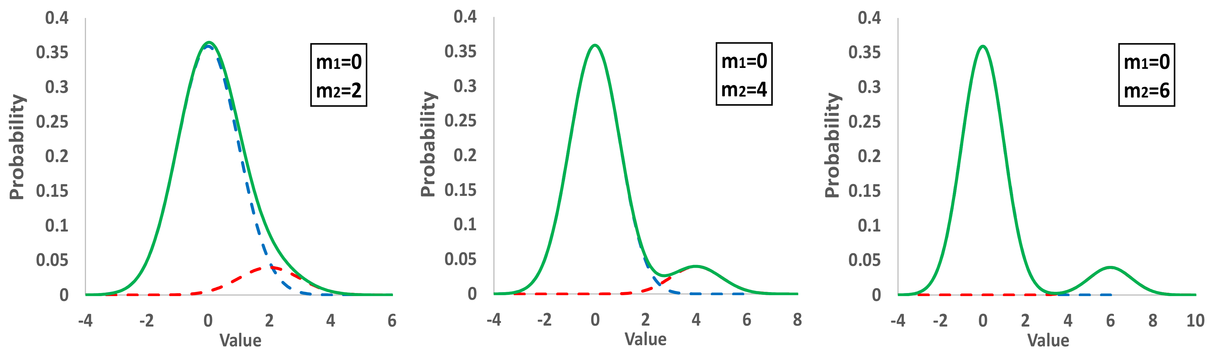
ISO 13258-2015 [14] (p. 10, Note 1) refers that a kernel density plot is functional in identifying bimodalities or lack of symmetry. This standard describes the algorithm to develop these plots in paragraph 10.3 [14] (pp. 32–33), and Figure 1 shows two examples of kernels plots of two 28-day strength tests performed during 2020. The software utilizes normal distributions and the nIQR as the standard deviation estimator to derive the kernels, as the standard recommends [14] (p. 32).

The results of each test belong to distributions that are difficult to disclose for participating laboratories, 11 to 13 per round. However, the results of all yearly tests are a population large enough to estimate the distribution. The algorithm achieves normalization by using the difference of the assigned value from the mean value of each participant, D_ij = x_ij − x_pt,j, where i is the participant and j is the round. Figure 2 depicts the kernel functions and the actual 28-day strength results for the 2019 and 2020 rounds.

The addition of one or two contaminating normal distributions to the main distribution effectively simulates such situations. The best-fitting mix of normal distributions, having the minimum distance from the kernel distribution, is also presented in Figure 2. The fraction of the surface of each distribution and the corresponding parameters have been computed using the Generalized Reduced Gradient non-linear regression technique, and their values are shown in

Table 1. Parameters of the normal distributions.

Parameter	2019	2020
Main distribution mean value, m1, MPa	0.00	0.04
Main distribution standard deviation, s1, MPa	1.24	1.46
Second distribution mean value, m2, MPa	2.51	4.00
Second distribution standard deviation, s2, MPa	0.90	0.70
Third distribution mean value, m3, MPa	−4.30	−3.60
Third distribution standard deviation, s3, MPa	0.90	0.70
Fraction of the main distribution, fr1	0.812	0.925
Fraction of the second distribution, fr2	0.107	0.019
Fraction of the third distribution, fr3	0.081	0.057
Distance of m1 and m2, |m2 − m1|/s1	2.0	2.7
Distance of m1 and m3, |m3 − m1|/s1	3.5	2.5

.

Using the subsequent two simple simulations, one can observe the impact of the secondary contaminating distributions on the main one:

(i)

The main normal distribution with m₁ = 0 and s₁ = 1 represents 90% of the population, while a secondary group representing the rest 10% has m₂ = 2s₁, 4s₁, 6s₁, and s₂ = s₁. The sum of the two populations results in a bimodal distribution.

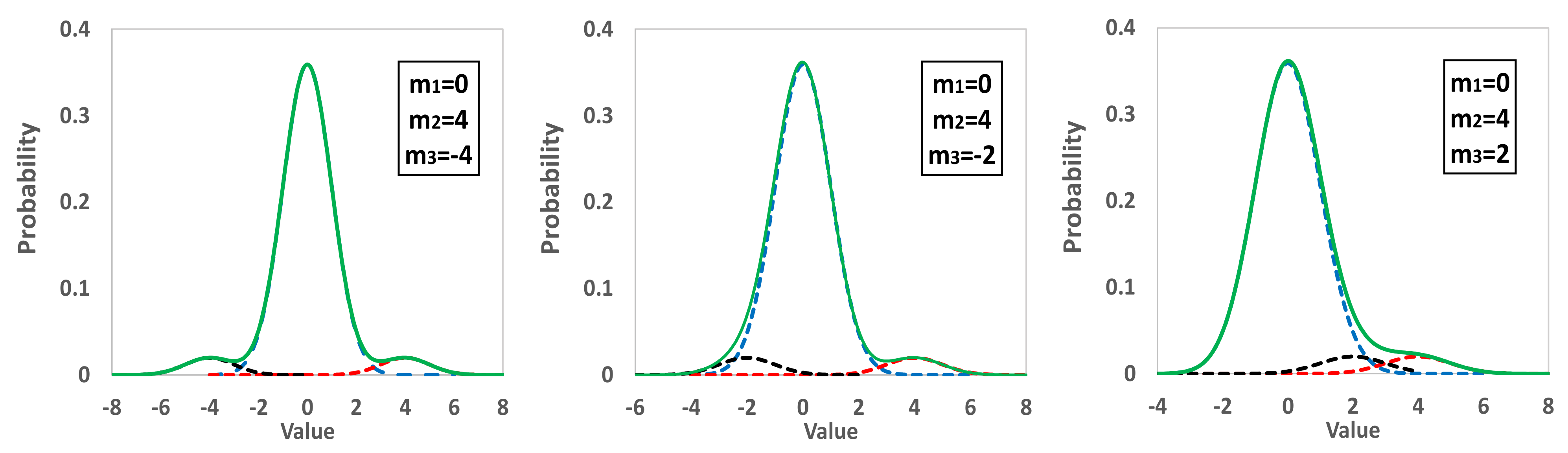
(ii)

The main distribution with m₁ = 0 and s₁ = 1 represents 90% of the population, a second one the 5% with m₂ = 4s₁, while a third distribution the rest 5% with m₃ = −4s₁, −2s₁, 2s₁. All the standard deviations are equal to one, and the derived distribution is trimodal.

(iii)

Figure 3 and Figure 4 demonstrate the results of these initial simulations, and one can recognize a lot of actual distributions obtained in proficiency testing.

2.2. Monte Carlo Simulations

The model developed utilizes the Monte Carlo approach to investigate and compare the robust methods used in the PT schemes. It assumes a default normal distribution of mean m₁ and standard deviation s₁, contaminated with one or two secondary distributions with mean values m₂ and m₃, respectively, and standard deviations equal to s₁. The following data are inputs and independent variables of the algorithm:

• Number of participating laboratories, N_lab;
• Number of replicate analyses per laboratory, N_rep;
• Repeatability standard deviation, s_r;
• Mean of the main normal distribution, m₁;
• Standard deviation of the main normal distribution, s₁;
• Mean and standard deviation of the second distribution, m₂, s₂;
• Population fraction of second distribution, fr₂;
• Mean and standard deviation of the third distribution, m₃, s₃;
• Population fraction of third distribution, fr₃;
• Number of iterations, N_iter;
• Number of simulations, N_s;
• Number of buckets to create histograms, N_b.

The Monte Carlo simulation initially selects a main normal distribution with mean value m₁ and standard deviation s₁ and adds two distributions contaminating the first one. The mean values of these two added populations are m₂ and m₃, their standard deviation s₂ = s₃ = s₁, the repeatability of each result is equal to s_r, and their fractions fr₂ and fr₃ correspondingly. Consequently, the fraction of the main population is fr₁ = 1 − fr₂ − fr₃. This approach manages to create three types of distributions: (a) if fr₂ = fr₃ = 0, a single normal distribution; (b) if fr₂ > 0 and fr₃ = 0, a bimodal population; (c) if fr₂ > 0 and fr₃ > 0, a trimodal population. The simulation assumes N_lab participating laboratories and selects for each laboratory’s result a random number, Rnd, between 0 and 1. If Rnd < fr₃, the result belongs to the third population. If fr₃ ≤ Rnd < fr₃ + fr₂, it belongs to the second population. If fr₃ + fr₂ ≤ Rnd, it is found in the main distribution. The mean value of each laboratory result is calculated by Equation (1):

$$X_i=Norm.Inv\left(m_k,s_k,Rn{d}_1\right)$$

(1)

where X_i is the mean value of the laboratory i, Norm.Inv is the inverse of the cumulative function of the normal distribution with mean value m_k, standard deviation s_k, and probability Rnd₁ which is a random number between 0 and 1. The index k is 1, 2, or 3 depending on the value of Rnd. The number of replicate analyses per laboratory is assumed to be always two. The same formula (1) applies to computing the value of each analysis by replacing: (a) m_k with X_i; (b) s_k with s_r; (c) Rnd₁ with Rnd₂ and 1-Rnd₂ for each calculation where Rnd₂ represents a random number between 0 and 1. Each simulation includes N_iter = 1000 iterations, and for each dataset, the software performs N_s = 25 simulations to compute the statistics of the randomly generated populations. The developed algorithm calculates the mean values, standard deviations, and the performance statistics shown in

Table 2. Classical and robust statistics.

Statistic	Applied Standard	Variable Name
Mean values
General mean	ISO 5725-2:1994, 7.4	GM1
Median value	ISO 13528:2015, C. 2.1	MED
Robust mean—Algorithm A with iterated scale	ISO 13528:2015, C. 3.1	Ax*
Hampel estimator for mean	ISO 13528:2015, C. 5.3.2	Hx*
Standard deviations
Scaled median absolute deviation	ISO 13528:2015, C. 2.2	MADe
Normalized interquartile range	ISO 13528:2015, C. 2.3	nIQR
Reproducibility standard deviation without outliers	ISO 5725-2:1994, 7.4	sRep
Robust standard deviation—Algorithm A with iterated scale	ISO 13528:2015, C. 3.1	As*
Robust standard deviation—Q method	ISO 13528:2015, C. 5.2.2	Hs*
Absolute Z factors
Z using MED, MADe	17043:2010. B3.1.3	Z_MADe
Z using MED, nIQR		Z_nIQR
Z using GM, sRep		Z_sRep
Z using Ax*, As*		Z_A
Z using Q/Hampel, Hx*, Hs*		Z_Hamp

¹ The abbreviation GM, used for general mean, should not be confused with that commonly used for GM-estimators (generalized M-estimators) described in [34].

, according to the analysis of ISO 13258-2015 [14] (pp. 52–62), ISO 5725-2:1994 [15] (pp. 10–14), and EN ISO/IEC 17043:2010 [1] (pp. 30–33). This table demonstrates the respecting clause of the standard applied as well as the variable name.

The outliers in the application of ISO 5725-2 for mean and reproducibility were determined using the Cochran’s and Grubbs’ tests: The first test was applied once, while the second one for the highest and lowest values. Tables 4 and 5 of ISO 5725-2 have critical values of the two outliers’ tests, up to a maximum number of participating laboratories N_lab = 40 [15] (pp. 21–22). The software used the following Equations (2) and (3) to compute the 1% critical values for any N_lab [35,36], which were also verified in case N_lab ≤ 40:

$$C_{crit}=\frac{1}{\left(1+\frac{N_{lab}-1}{1+F.Inv\left(\frac{a}{N_{lab}},N_{rep}-1, \left(N_{lab}-1\right)· \left(N_{rep}-1\right)\right)}\right)}$$

(2)

$$G_{crit}=\frac{\left(N_{lab}-1\right)·t.Inv\left(\frac{a}{N_{lab}},N_{lab}-2\right)}{\sqrt{N_{lab}}}·\sqrt{\frac{1}{N_{lab}-2+t.Inv{\left(\frac{a}{N_{lab}},N_{lab}-2\right)}^2}}$$

(3)

where C_crit, G_crit are the critical values of Cochran’s and Grubbs’ tests, correspondingly, for α = 0.01, and t.Inv, F.Inv are the inverse functions of the Student and Fisher distributions. The software applied the robust algorithms described in Annex C of ISO 13528:2015 to calculate the population means and standard deviations provided in Table 2. The Z-factor for laboratory value X_i, assigned value x_PT, and population standard deviation σ_PT is determined using Equation (4) according to 17043:2010 [1] (p. 30):

$$Z=\frac{X_i-x_{PT}}{{\sigma }_{PT}}$$

(4)

3. Comparisons of Population Mean Values and Standard Deviations

3.1. Initial Implementation of Simulations

The Monte Carlo simulation was first applied to a wide range of participating laboratories and a narrow range for the other independent variables presented in Section 2.2. In Section 2.1, one can see kernel density plots of actual 28-day strength results and computed parameters of the mix of three Gaussian distributions. The initial implementation of the simulation uses long-term 28-day strength data for the mean value and the variance of the normally distributed main population. Afterwards, the simulator adds a contaminating population following the same distribution with the main one and differing in mean value from it. The settings used were: N_lab = 15, 20, 30, 40, 60, 80, 100, 150, 200, 300, 400; N_rep = 2; s_r = 0.40, 0.01 MPa; m₁ = 50.8 MPa; s₁ = 1.76 MPa; m₂ = 52.6, 54.4, 56.2 MPa; s₂ = 1.76 MPa; fr₂ = 0, 0.05, 0.10; fr₃ = 0; N_iter = 1000; N_s = 25; N_b = 20; The mean value m₁ = 50.8 MPa is the average of the population means of 81 rounds the PT scheme performed from 2012 to 2020 using the Hampel estimator. The s₁ = 1.76 and s_r = 0.4 represent the average between laboratories’ standard deviation, s_L, and the repeatability for the same rounds. Q-method uses all the results of each laboratory, while the other robust methods use the mean value of each participant. By applying two s_r values, the simulation investigates the possible impact of the repeatability on the Q-method results. The settings selected correspond to bimodal distributions, where the mean of the second population m₂ is in distances of 1.02 (=1.8/1.76), 2.05, and 3.07 from the mean m₁ in s₁ units.

Table 3. Average and standard deviation of the mean values.

	GM	MED	Ax*	Hx*	GM	MED	Ax*	Hx*	GM	MED	Ax*	Hx*	GM	MED	Ax*	Hx*
Nlab	Mean values, mav				Standard deviations, sav				Mean values, mav				Standard deviations, sav
	m2 = 52.6 MPa, mtot = 50.98 MPa, fr2 = 0.10								m2 = 54.4 MPa, mtot = 51.16 MPa, fr2 = 0.10
15	50.98	50.96	50.97	50.97	0.48	0.59	0.50	0.50	51.16	51.05	51.09	51.09	0.54	0.63	0.55	0.55
20	50.98	50.96	50.97	50.97	0.41	0.50	0.42	0.42	51.15	51.04	51.09	51.09	0.47	0.53	0.47	0.47
30	50.97	50.96	50.97	50.97	0.33	0.41	0.34	0.34	51.15	51.04	51.09	51.09	0.38	0.44	0.38	0.38
40	50.98	50.96	50.97	50.97	0.28	0.34	0.28	0.28	51.15	51.03	51.08	51.08	0.31	0.36	0.31	0.31
60	50.98	50.96	50.97	50.97	0.23	0.28	0.23	0.23	51.15	51.03	51.09	51.09	0.26	0.30	0.26	0.26
80	50.98	50.96	50.97	50.97	0.21	0.25	0.21	0.21	51.16	51.03	51.09	51.09	0.23	0.27	0.23	0.23
100	50.98	50.96	50.97	50.97	0.18	0.23	0.19	0.19	51.16	51.03	51.09	51.09	0.21	0.24	0.21	0.21
150	50.98	50.96	50.97	50.97	0.15	0.19	0.15	0.15	51.16	51.04	51.09	51.09	0.17	0.20	0.17	0.17
200	50.98	50.96	50.97	50.97	0.13	0.16	0.13	0.13	51.16	51.03	51.09	51.09	0.15	0.17	0.15	0.15
300	50.98	50.96	50.97	50.97	0.11	0.13	0.11	0.11	51.16	51.03	51.09	51.09	0.12	0.14	0.12	0.12
400	50.98	50.96	50.97	50.97	0.09	0.11	0.09	0.09	51.16	51.03	51.09	51.09	0.10	0.12	0.10	0.10
	m2 = 56.2 MPa, mtot = 51.34 MPa, fr2 = 0.10
15	51.31	51.06	51.15	51.15	0.63	0.64	0.59	0.59
20	51.31	51.06	51.16	51.15	0.55	0.54	0.51	0.51
30	51.32	51.05	51.15	51.15	0.45	0.44	0.41	0.41
40	51.32	51.05	51.15	51.15	0.38	0.37	0.34	0.34
60	51.33	51.05	51.14	51.14	0.31	0.31	0.28	0.28
80	51.33	51.05	51.14	51.14	0.27	0.27	0.25	0.25
100	51.33	51.05	51.14	51.14	0.24	0.25	0.23	0.23
150	51.33	51.05	51.14	51.14	0.20	0.20	0.18	0.18
200	51.34	51.05	51.14	51.14	0.17	0.17	0.16	0.16
300	51.34	51.05	51.14	51.14	0.14	0.14	0.13	0.13
400	51.34	51.05	51.14	51.14	0.12	0.12	0.11	0.11

presents the average values and standard deviations of mean values of the population, m_av and s_av, correspondingly, calculated from Equations (5) and (6), for fr₂ = 0.10:

$$m_j={{\displaystyle \sum }}_{i=1}^{N_{iter}}{m}_{ij}/N_{iter}, s{m}_j=\sqrt[]{\frac{{{\displaystyle \sum }}_{i=1}^{N_{iter}}{\left(m_{ij}-m_j\right)}^2}{N_{iter}-1}} j=1 to N_s$$

(5)

$$m_{av}={{\displaystyle \sum }}_{j=1}^{N_s}{m}_j/N_s, s_{av}={{\displaystyle \sum }}_{j=1}^{N_s}s{m}_j/N_s$$

(6)

where m_ij are the mean values of each N_lab, m_j is the mean value, and sm_j is the standard deviation of m_ij for the simulation j.

For comparison reasons, the mean value of the bimodal distribution is provided, computed from Equation (7):

$$m_{tot}=\left(1-f{r}_2\right)·m_1+f{r}_2·m_2$$

(7)

The four estimators of the mean population value are approximately equal for m₂ = 52.6 MPa and close to m₁. For larger values of m₂, the GM estimator starts to be higher than the others and approaches the m_tot value, meaning that when m₂ > m₁ + s₁, GM is not a robust estimator. The three robust estimators provide a good approximation of m₁, but the median value shows a higher variance, especially for smaller N_lab.

The average values and standard deviations of the population standard deviations are computed by Equations (8) and (9):

$$s_j={{\displaystyle \sum }}_{i=1}^{N_{iter}}{s}_{ij}/N_{iter}, s{s}_j= \sqrt[]{\frac{{{\displaystyle \sum }}_{i=1}^{N_{iter}}{\left(s_{ij}- s_j\right)}^2}{N_{iter}-1}} j=1 to N_s$$

(8)

$$m_{std}={{\displaystyle \sum }}_{j=1}^{N_s}{s}_j/N_s, s_{std}={{\displaystyle \sum }}_{j=1}^{N_s}s{s}_j/N_s$$

(9)

where s_ij is the standard deviation of each N_lab, s_j is the mean value, and ss_j is the standard deviation of s_ij for the simulation j. Figure 5 and Figure 6 show the average values and standard deviations of the population standard deviation for fr₂ = 0 and 0.10, from which one can conclude the following:

(i)

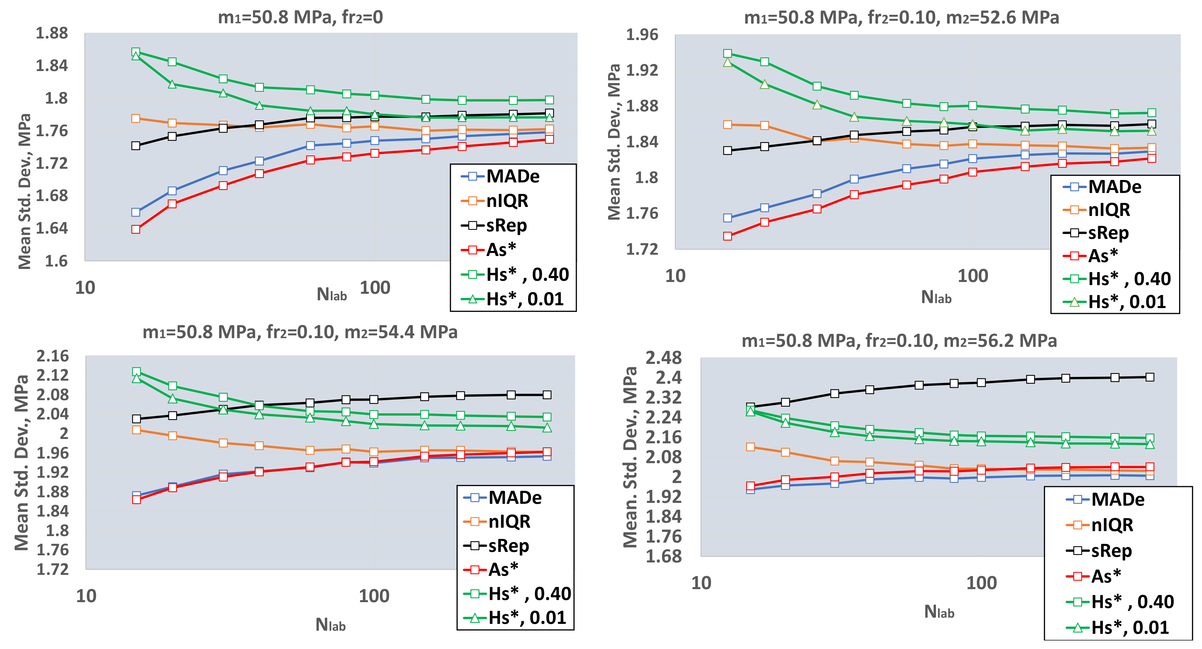
For a large number of laboratories, N_lab ≥ 200, the mean values of the estimators converge to different values. MADe, nIQR, and As* approach approximately the same value, while the convergence value of Hs* is higher for both repeatability values. The sRep is between these values for fr₂ = 0 and m₂ = m₁ + s₁ and becomes higher from both for m₂ ≥ m₁ + 2s₁. The above proves that this estimator is not resistant to outliers. The high value of sRep for high m₂ can underestimate the number of laboratories with |Z|>3.

(ii)

All functions between estimators and N_lab are monotonic. Those of MADe, sRep, and As* are increasing and those of nIQR and Hs* are decreasing. The MADe and As* low values for small N_lab may overestimate |Z| values. The current analysis shows MADe and As* are the lowest among robust estimators for small N_lab.

(i)

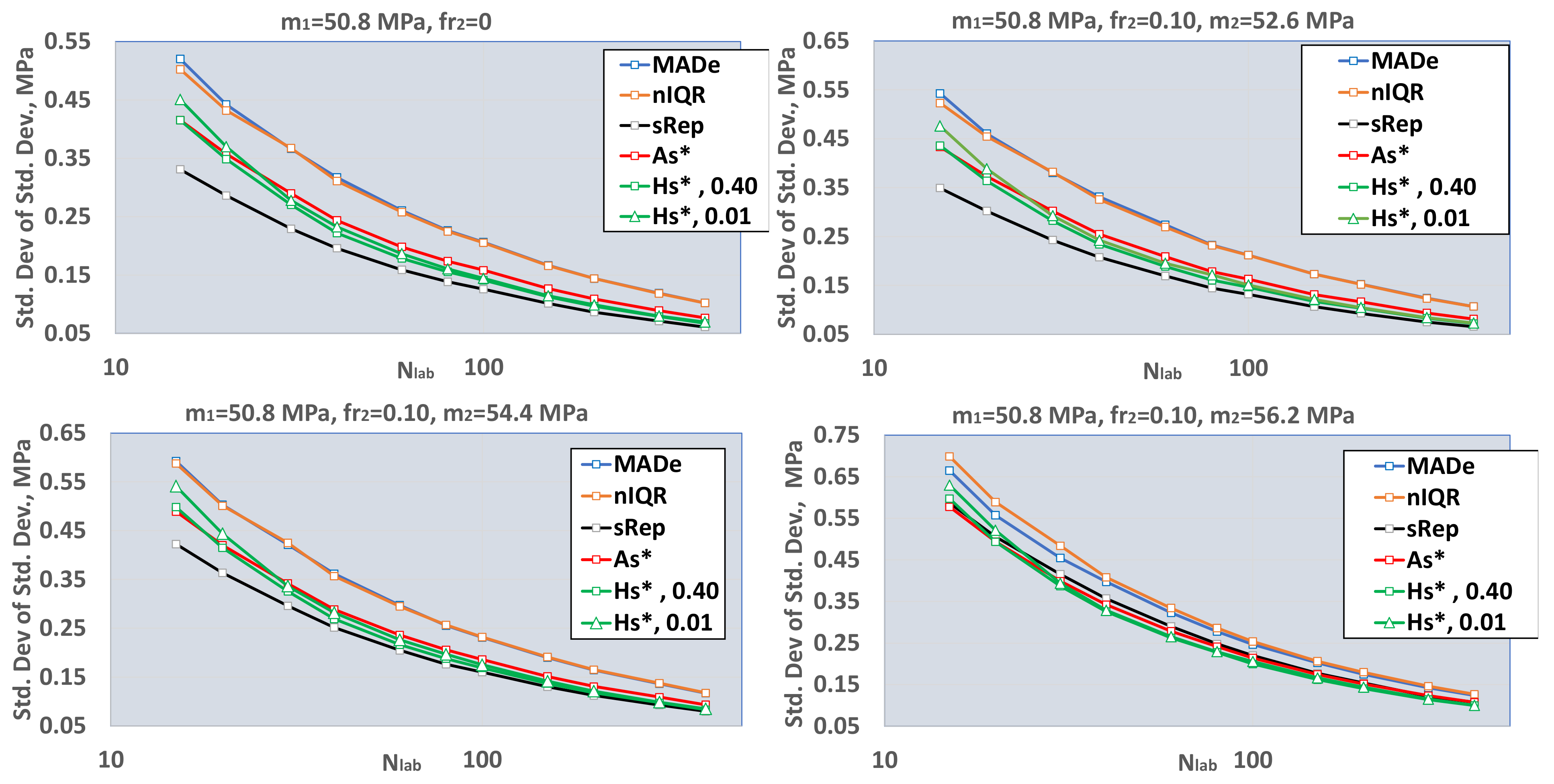
Increasing the m₂ value, the average value and standard deviation of the population standard deviation also increase.

(ii)

The standard deviation of the population standard deviation of MADe and nIQR is continuously higher than the respecting values of the other three estimators. The above is in good agreement with paragraph 6.5.2 of ISO 13253:2015 [14] (p. 12), which further notes that more sophisticated robust estimators provide better performance for approximately normally distributed data, while retaining much of the resistance to outliers offered by MADe and nIQR.

(iii)

The average standard deviation of the Q method with s_r = 0.40 is a little higher than that with negligible repeatability, s_r = 0.01. Further simulations will utilize only s_r = 0.01 for the Q method to be comparable with the other robust methods.

Figure 7 depicts the distributions of the population standard deviations for one simulation with N_iter = 10000, N_s = 1, s_r = 0.01, m₂ = 52.6 MPa, 56.2 MPa, fr₂ = 0.10, N_b = 20, and N_lab = 20, 40, from where one can observe:

(i)

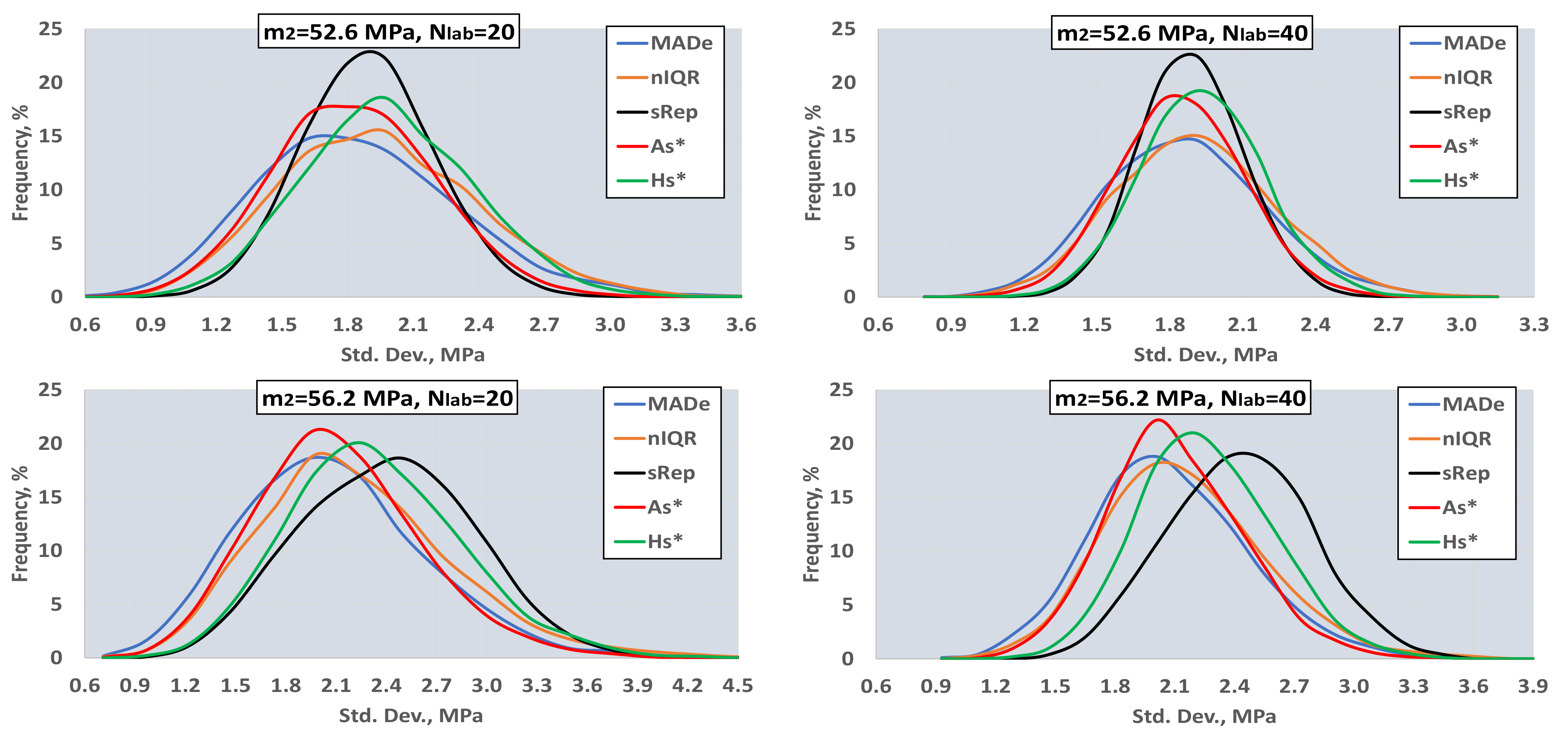
All distributions are approximately symmetric around their mean;

(ii)

The variance of MADe and nIQR is greater than that of other estimators, especially for lower values of m₂.

3.2. Determining the Best Estimators for a Small Number of Laboratories

As proved in Section 3.1, the estimators GM and sRep are not resistant to outliers. The problem needing a solution is the determination of the best robust estimators based on the number of participants and the actual distribution of the results. The proposed method uses the absolute value of the Z-factor given by Equation (4). According to EN ISO/IEC 17043:2010 [1] (p. 32), if |Z|>3, the laboratory performance is unsatisfactory, and the result is an outlier. Using robust estimators to detect the outliers indicates that the approach is nonparametric. Supposing that a distribution of a large number of results, actual or simulated, contains Zu% non-satisfactory results, the question is which robust estimators best approach these values when the number of labs is N_lab. The developed algorithm applies the Monte Carlo simulation presented in Section 2.2 and follows the subsequent steps:

(i)

It creates a main normal distribution D₁ with mean value m₁ and standard deviation s₁ and two contaminating distributions D₂, D₃ with mean values m₂, m₃, and standard deviations s₂ = s₃ = s₁.

(ii)

The fractions of the contaminating distributions are fr₂ and fr₃, and, depending on these two values, the total distribution can be unimodal, bimodal, or trimodal.

(iii)

The mean values m₂ and m₃ differ by an integer number of standard deviations s₁ from m₁, n₂ and n₃, shown in Equation (10). In the case of trimodal distribution, if n₂·n₃ > 0, then D₂ and D₃ are both to the same side of the D₁. Otherwise, one is to the left and the other to the right of D₁. Figure 4 of Section 2.1 depicts such distributions:

$$m_2=m_1+n_2·s_1 ,m_3=m_1+n_3·s_1 with n_2\ge 0 and n_3\ge 0 or n_3<0$$

(10)

(iv)

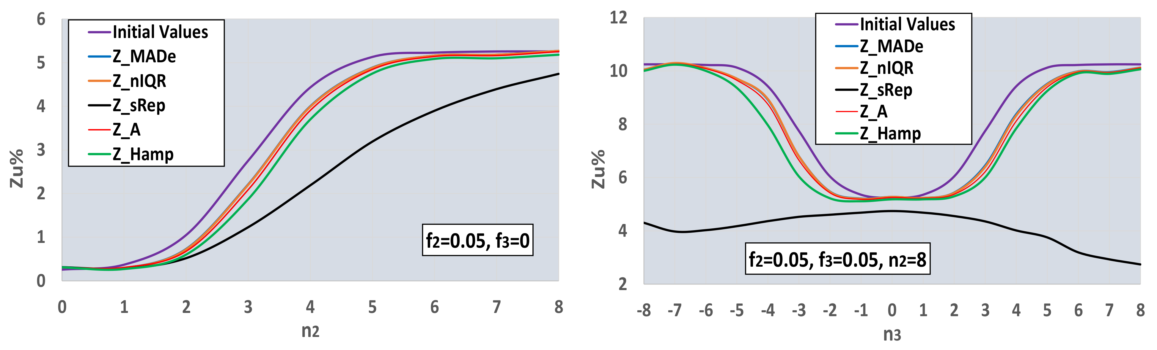
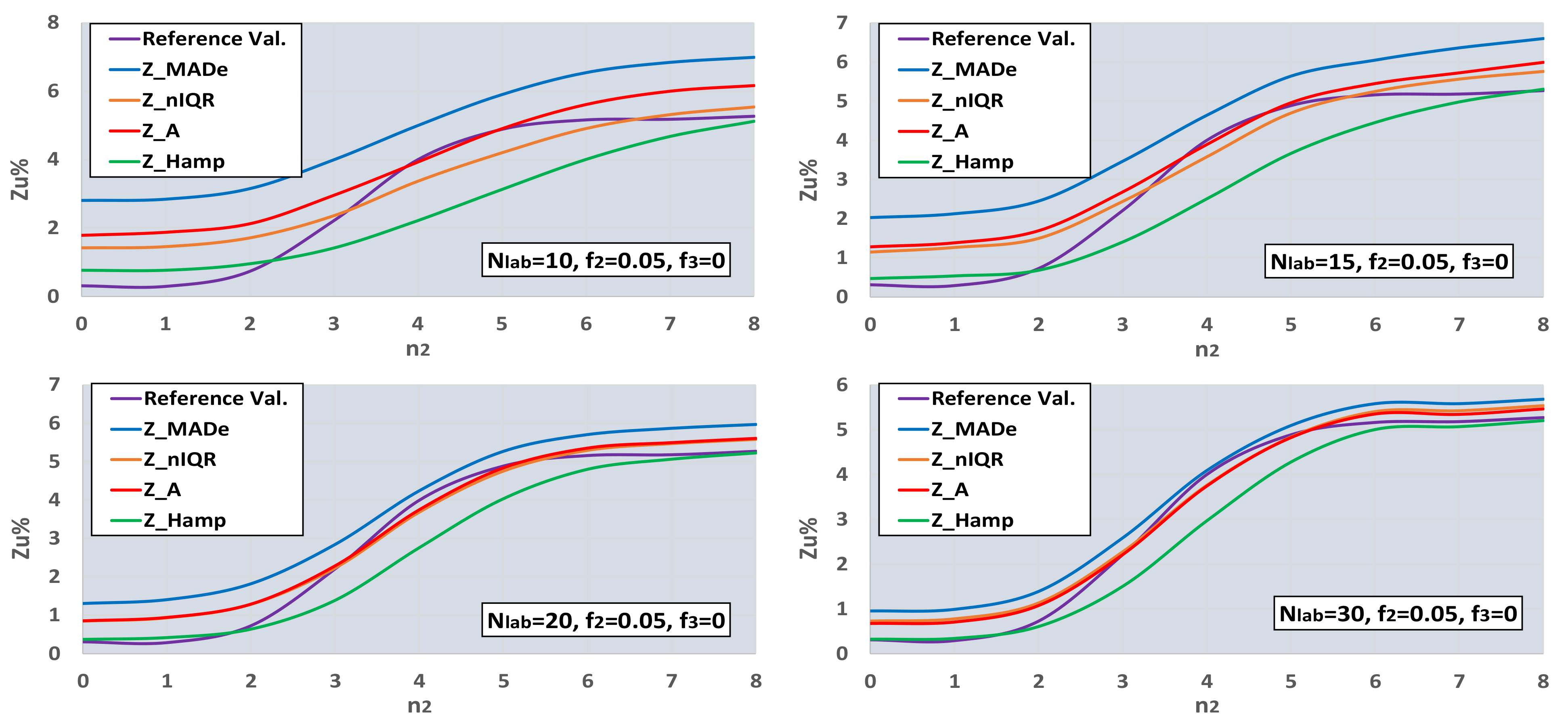
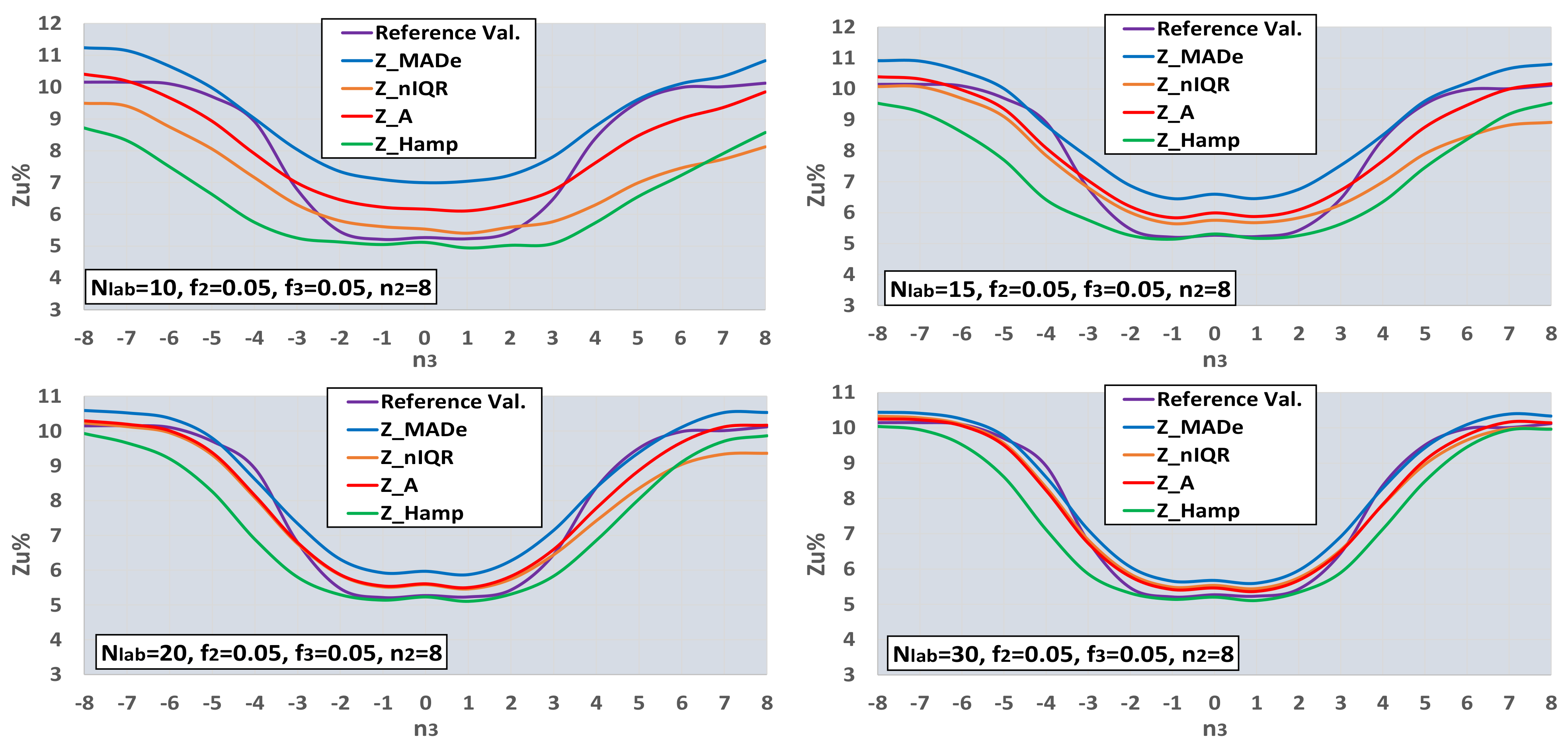
According to the values of fr₂, fr₃, n₂, and n₃, the software calculates the values of Zu%, which are unsatisfactory, compared to the normal distribution function with mean and standard deviation m₁ and s₁, correspondingly. These values are the initial values. For example, if fr₂ = 0.1, fr₃ = 0, and n₂ = 3, then Zu% = 0.24 (from D₁) + 5.0 (from D₂) = 5.24.

(v)

The algorithm calculates all the estimators for the mean and standard deviation shown in Table 1 and the Zu% for the absolute values of the five Z-factors presented in the same table using a N_lab = 400. Afterwards, it calculates the average of Zu% for N_iter = 400 and N_s = 4. The other settings are the ones shown in

Table 4. Simulation settings.

Setting	Value
Nlab	10, 15, 20, 30 and 400 1
Nrep	2
sr, MPa	0.01
m1, MPa	50
s1, MPa	1
m2, MPa	m2 = m1 + n2·s1, n2 = 1 to 8 and step 1
fr2	0, 0.025, 0.05, 0.075, 0.1 2
m3, MPa	m3 = m1 + n3·s1, n3 = −8 to 8 and step 1
fr3	0, 0.025, 0.05
s2, s3, MPa	1
Niter	1000
Ns	25

¹ If N_lab = 400, then the N_s = 4. ² If fr₃ = 0, then the maximum value of fr₂ is 0.1. Otherwise fr_2Max = 0.075 and fr₂ + fr₃ ≤ 0.1.

. For this number of participants, all estimators converge to their final value. Figure 8 illustrates the procedure.

(vi)

The Zu% of each of the five Z-factors are compared with the initial results of step (iv). Those results closest to the initial ones are the reference values and represent the best estimation of the robust methods in approaching the unsatisfactory results calculated using the main distribution.

(vii)

The simulations implemented all the settings shown in Table 4 for participants up to 30. The populations correspond to unimodal, bimodal, and trimodal distributions with a maximum total fraction of secondary distributions up to 0.1. The coefficient of variation of the main distribution is 2% (=1/50 × 100).

(viii)

The software performs N_iter iterations and N_s simulations for each N_lab. For all these results, the average of each one of the five Zu% is calculated. These results are compared with each other and with reference values. The estimator providing the closest value to the reference value for each parameter set is optimal.

Figure 8 proves that the calculation of Zu% using Z_sRep results leads to a severe underestimation of the percentage of the unacceptable Z-factors, compared to all the other estimators. The Zu% values derived from the robust estimators are close to each other and not far from the initial values computed using the main normal distribution. The Zu% values calculated by Z_Hamp are slightly worse than the values calculated by Z_MADe, Z_nIQR, and Z_A. The simulator compared all Zu% for N_lab = 400 and all the other settings of Table 4. It found that the closest estimator of unacceptable Z-factors to the estimation based on the main normal distribution is the Z_MADe in 95% of cases. For this reason, it uses the values of this estimator as a reference in further calculations. However, this does not mean that the Z_MADe is consistently the optimal estimator for a small number of participants.

Figure 9 and Figure 10 depict the Zu% for the reference values and all the robust estimators for selected bimodal and trimodal distributions of the results’ population. In both figures, the number of labs is from 10 to 30.

One can observe that the optimal estimator is a function of both the number of deviations and the number of labs. In bimodal distribution and for the given f₂, Z_Hamp is optimal for n₂ ≤ 2 and n₂ ≥ 6, depending on the N_lab value. Z_MADe is more efficient for N_lab ≥ 20 and n₂ = 4, while for the other values of n₂ and N_lab, the optimal estimators are Z_nIQR and Z_A. The trimodal distributions of Figure 10 contain two bimodal distributions in the case n₃ = 0 and 8. For the given value of n₂, Z_Hamp is more efficient in the center for −2 ≤ n₃ ≤ 2. Z_A and Z_nIQR are optimal in the two side zones for n₃ ≤ −6 and n₃ ≥ 7 and n₃ = −3, n₃ = 3. Finally, Z_MAde is the closest estimator to the reference values in the two intermediate zones for −5 ≤ n₃ ≤ −4 and 4 ≤ n₃ ≤ 6. The conclusion from the processing so far is that there is no generally optimal robust estimator, but its choice depends on the type of population distribution and its variance.

4. Optimal Robust Estimators for a Limited Number of Participants

4.1. Use of a Normal Distribution Mix

The application of steps (i)–(viii) of 3.2 for the full range of N_lab, n₂, n₃, fr₂, and fr₃ of Table 4 leads to a complete and exhaustive evaluation of the optimal robust estimator of the percentage of unacceptable results for each set of the mentioned settings and guides a PT scheme expert on which estimator to choose. The core of such an option for an actual PT is to disclose the distribution of results using the kernel plots and to fit a mixture of normal distributions into it, as described in Section 2.1. If the PT scheme organizer executes the test several times a year, selecting the results of the last and several recent rounds to generate the kernel plots is preferable. The last results have a significant probability of belonging to a population similar to the recent results’ population, especially if the same or almost the same laboratories participate. On the contrary, if the PT scheme expert would use only the last round to build the distribution, the parameters could have severe uncertainty due to the small number of participants.

Figure 11 shows the optimal robust estimators of Zu% for the bimodal distributions and the settings of Table 4. For f₂ = 0.025, the Q/Hampel estimator is predominant for most of the n₂ values, and only for n₂ = 4 method A and MED-nIQR are optimal. By increasing f₂, Q/Hampel remains optimal for n₂ ≤ 2, and its performance gradually decreases to high values of n₂. For f₂ = 0.05, method A and MED-nIQR predominate for 3 ≤ n₂ ≤ 6. As f₂ increases, MED-MADe becomes optimal near the mid-range of n₂, while the optimal Z_A move to the right, replacing Z_nIQR and Z_Hamp.

Figure 12, Figure 13, Figure 14 and Figure 15 depict the optimal estimators of Zu% for the trimodal distributions and all the combinations of f₂ and f₃ with f₂ + f₃ ≤ 0.10. For f₂ + f₃ = 0.05, Q/Hampel is optimal in the center (−3 ≤ n₃ ≤ 3) and in the two sides (n₃ ≤ −6, n₃ ≥ 6) for low and high n₂ values. Method A and MED-nIQR are highly performing in the remaining area of n₂, n₃. These results agree with those of Figure 11. For f₂ + f₃ = 0.075, Q/Hampel is optimal mainly in the center (−2 ≤ n₃ ≤ 2) for low and high n₂ values. MED-MADe shows the higher performance for the two mid-ranges of n₃ (n₃ = −4, −5, and n₃ = 4, 5) while method A and MED-nIQR remain optimal in the remaining area. For f₂ + f₃ = 0.10, the area covered by optimal Z_MADe is larger, replacing Z_A and Z_nIQR. Especially for f₂ = 0.05 and f₃ = 0.05, the region of optimal Z_Hamp becomes narrower, replaced mainly by Z_nIQR. Figure 11, Figure 12, Figure 13, Figure 14 and Figure 15 are suitable for practical reasons because they allow the PT scheme expert to select the proper robust estimator to evaluate the unsatisfactory results when the number of participants is between 10 and 30 with the underlying assumption that the main distribution presents a coefficient of variation ~2. Rounding to the values given in these figures is necessary for the number of labs and the f₂ and f₃ fractions calculated from the actual distribution.

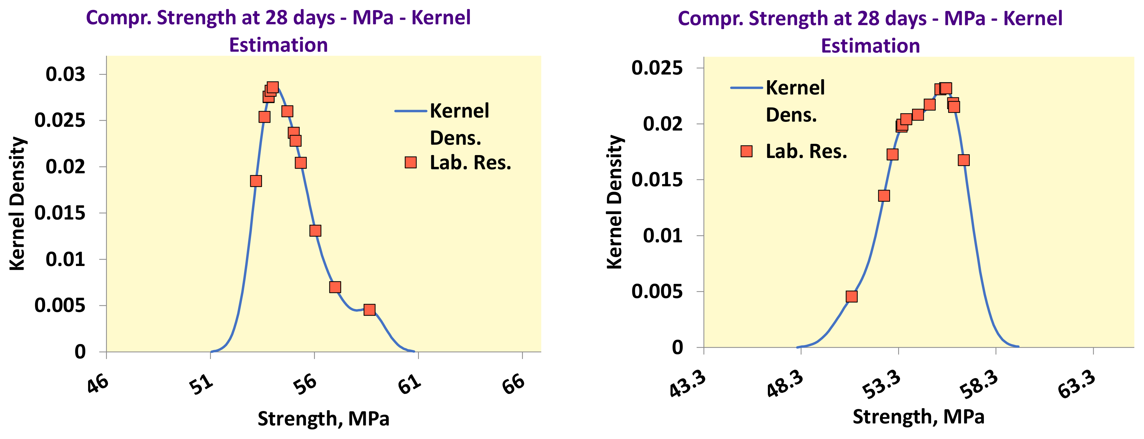
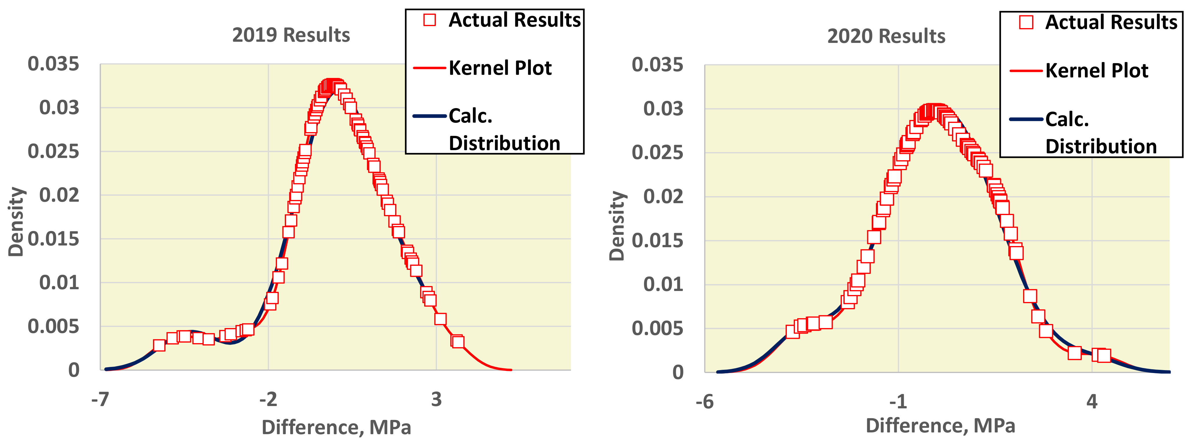
4.2. Use of Kernel Density Plots

Using the methods described in Section 2.1 and Section 3.2, we provide a generalized algorithm in determining the optimal robust estimators using actual results. The description of the algorithm follows using the practical example of the mentioned EUROCERT PT scheme. In that particular PT example, the organizer performs the 28-day strength test 9 times a year. The proposed algorithm implements the kernel density plot of each round, including the last test and the previous eight. For a small number of participants and several repeats of the test during the year, the estimated distribution using moving time horizon results should be closer to the real one than taking into account the limited number of the last round’s results. The algorithm performs normalization using the formula D_ij = x_ij − x_pt,j, described already in Section 2.1, before building the kernel density plot. It then assumes a main normal distribution. The addition of one or two contaminating normal distributions to the main follows, and the best-fitting mix of them, having the minimum distance from the kernel plot, is computed via non-linear regression. The values of m₁, m₂, m₃, s₂, s₃, f₂, and f₃ are the outputs of this process. Afterwards, the algorithm applies steps (i) to (viii) of Section 3.2 and determines the optimal estimator.

Table 5. Normal distribution parameters and optimum robust estimators for 18 consecutive 28-day strength tests.

	Code
	012019	022019	032019	042019	052019	062019	092019	102019	112019
Count	1	2	3	4	5	6	7	8	9
Nlab average	12	12	13	13	13	13	12	13	13
m1, MPa	0.12	0.09	0.03	0.05	0.12	0.07	0.12	0.1	-0.02
s1, MPa	1.48	1.56	1.59	1.64	1.51	1.37	1.46	1.48	1.23
f2	0.024	0.015	0.019	0.017	0.015	0.036	0.015	0.033	0.105
m2, MPa	4.55	4.5	5.19	5.28	5.36	3.75	5.34	4	2.46
s2, MPa	0.67	0.82	0.74	0.63	0.52	1.45	0.49	1.36	0.85
f3	0.101	0.08	0.044	0.053	0.08	0.074	0.06	0.056	0.081
m3, MPa	−3.52	−3.51	−4.14	−4.31	−3.9	−3.96	−4.16	−4.5	−4.32
s3, MPa	1.15	1.13	0.8	0.88	1.01	0.93	0.96	0.88	0.99
$\left(m_2-m_1\right)/s_1$	2.99	2.83	3.25	3.19	3.47	2.69	3.58	2.64	2.02
$\left(m_3-m_1\right)/s_1$	−2.46	−2.31	−2.62	−2.66	−2.66	−2.94	−2.93	−3.11	−3.50
f2 + f3	0.125	0.095	0.063	0.070	0.095	0.110	0.075	0.089	0.186
Optimal	Z_Hamp	Z_Hamp	Z_nIQR, Z_Hamp	Z_nIQR, Z_Hamp	Z_nIQR	Z_nIQR	Z_nIQR, Z_A	Z_nIQR	Z_nIQR
Status	N/A	OK	OK	OK	OK	OK	OK	OK	N/A
Figure		14	13	13	14	14	13	13
Nlab, n2, n3		10, −2, 3	15, −3, 3	15, −3, 3	15, −3, 3	15, −3, 3	10, −3, 4	15, −3, 3
	Code
	012020	022020	032020	042020	052020	062020	092020	102020	112020
Count	11	12	13	14	15	16	17	18	19
Nlab average	12	12	12	12	12	12	12	12	12
m1, MPa	−0.14	0.43	−0.28	−0.3	−0.37	−0.41	0.08	0.16	0.04
s1, MPa	1.28	1.51	0.73	0.71	0.71	0.78	1.26	1.43	1.5
f2	0.142	0.154	0.171	0.196	0.367	0.375	0.08	0.045	0.015
m2, MPa	2.31	−0.58	1.47	1.42	1.25	1.34	2.94	1.43	4.7
s2, MPa	0.84	0.6	0.62	0.61	0.9	0.9	1.3	2.63	0.8
f3	0.059	0.068	0.383	0.389	0.166	0.151	0.081	0.061	0.041
m3, MPa	−4.27	−4.04	−0.16	−0.23	−2.63	−3.03	−3.54	−3.61	−3.69
s3, MPa	1.01	1.1	2.49	2.46	1.52	1.29	0.82	0.69	0.53
$\left(m_2-m_1\right)/s_1$	1.91	−0.67	2.40	2.42	2.28	2.24	2.27	0.89	3.11
$\left(m_3-m_1\right)/s_1$	−3.23	−2.96	0.16	0.10	−3.18	−3.36	−2.87	−2.64	−2.49
f2 + f3	0.201	0.222	0.554	0.585	0.533	0.526	0.161	0.106	0.056
Optimal	Z_nIQR	Z_nIQR	Z_nIQR	Z_nIQR	Z_nIQR	Z_nIQR, Z_Hamp	Z_Hamp	Z_Hamp	Z_Hamp
Status	N/A	N/A	N/A	N/A	N/A	N/A	N/A	Not OK	OK
Table									13
Nlab, n2, n3									10, −2, 3

shows the parameters of the distributions for 18 consecutive 28-day strength tests, along with the average N_lab and the optimal robust estimators of Zu% using the mentioned algorithm. If a second estimator differs from the reference value less than 5% from the respecting distance of the optimal one, the estimator is also optimal. If f₂ + f₃ is lower than or close to 0.1, the algorithm compares the optimal estimator with the one predicted in Figure 11, Figure 12, Figure 13, Figure 14 and Figure 15. In the case of a positive check, the table indicates the values of N_lab, n₂, and n₃ of the corresponding figure. In 8 out of the 9 cases where f₂ and f₃ meet the conditions of Figure 11, Figure 12, Figure 13, Figure 14 and Figure 15, the prediction of these figures is correct, although the standard deviations are not equal and s₁ ≈ 1.5 MPa. The long-term average of the populations’ means is around 50 MPa, as reported in 3.1, concluding that the coefficient of variation of D₁ is about 3%. That means that the results of Figure 11, Figure 12, Figure 13, Figure 14 and Figure 15 obtained for a variation coefficient of 2% are robust for values up to 3%. Table 5 shows that the algorithm is suitable for an expanded range of the secondary populations’ fractions and unequal standard deviations s₁, s₂, and s₃.

Figure 16 depicts all the Zu% results, including the optimal ones, Z_Optim, leading to the following conclusions for N_lab = 12–13:

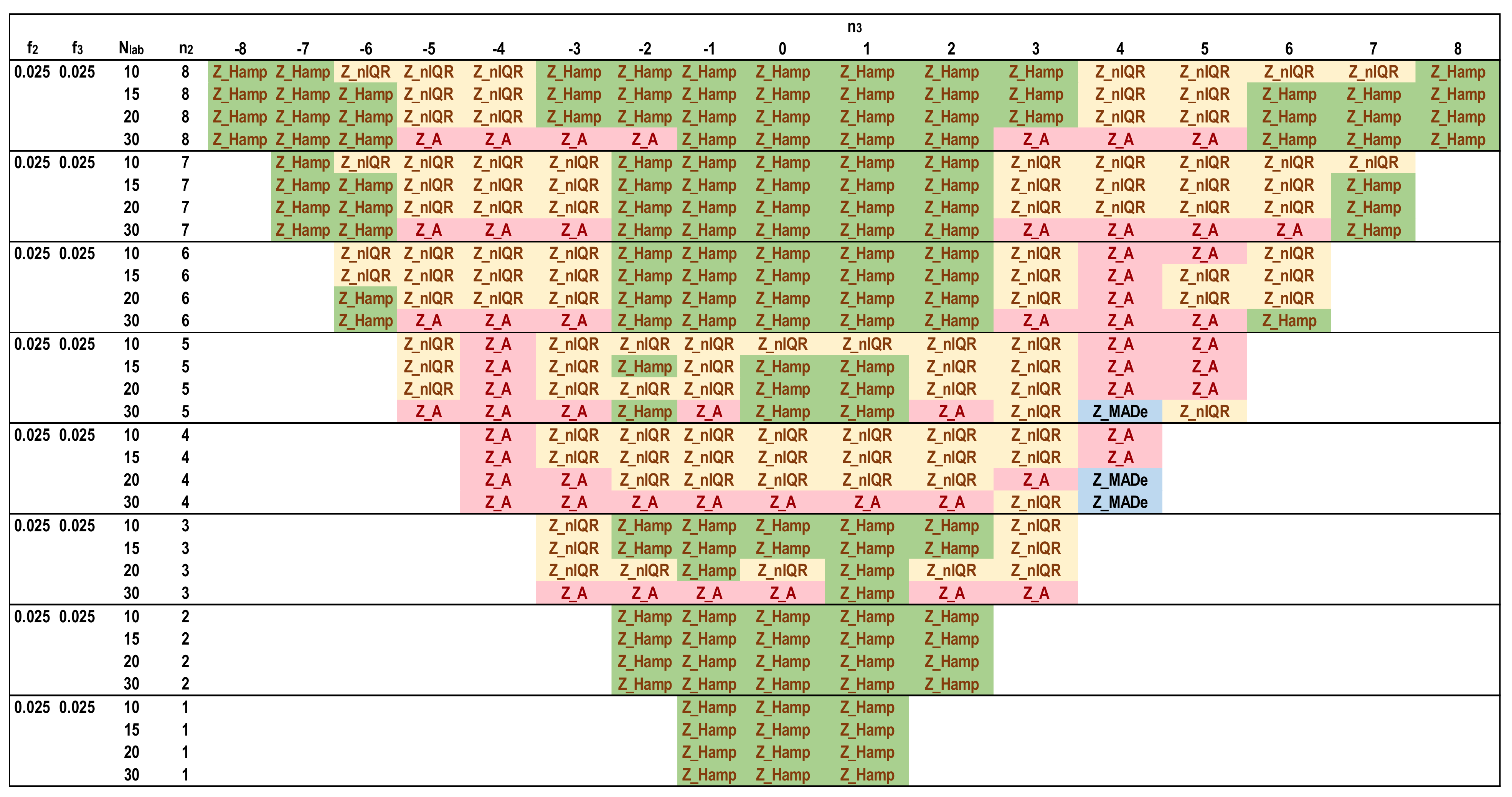
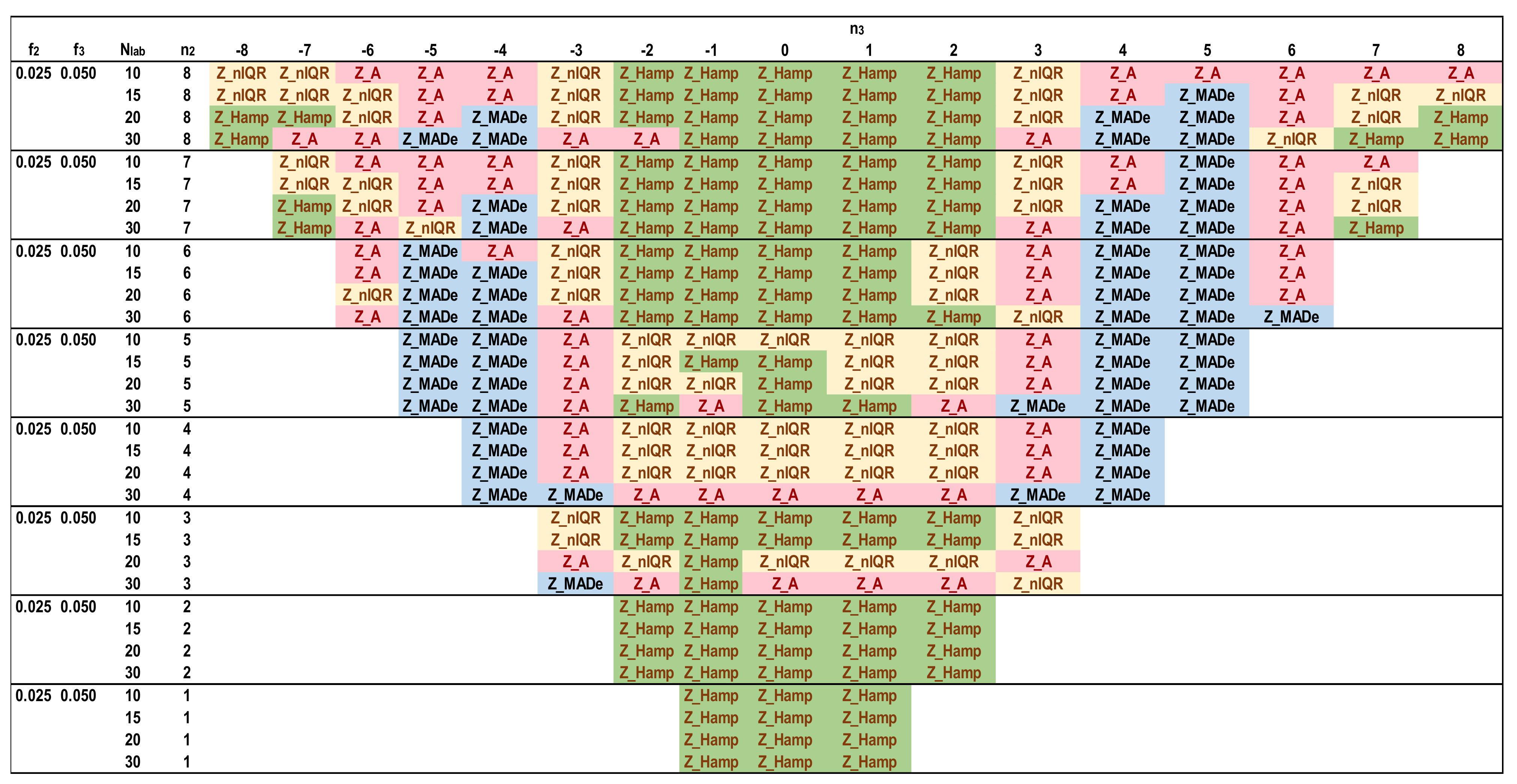
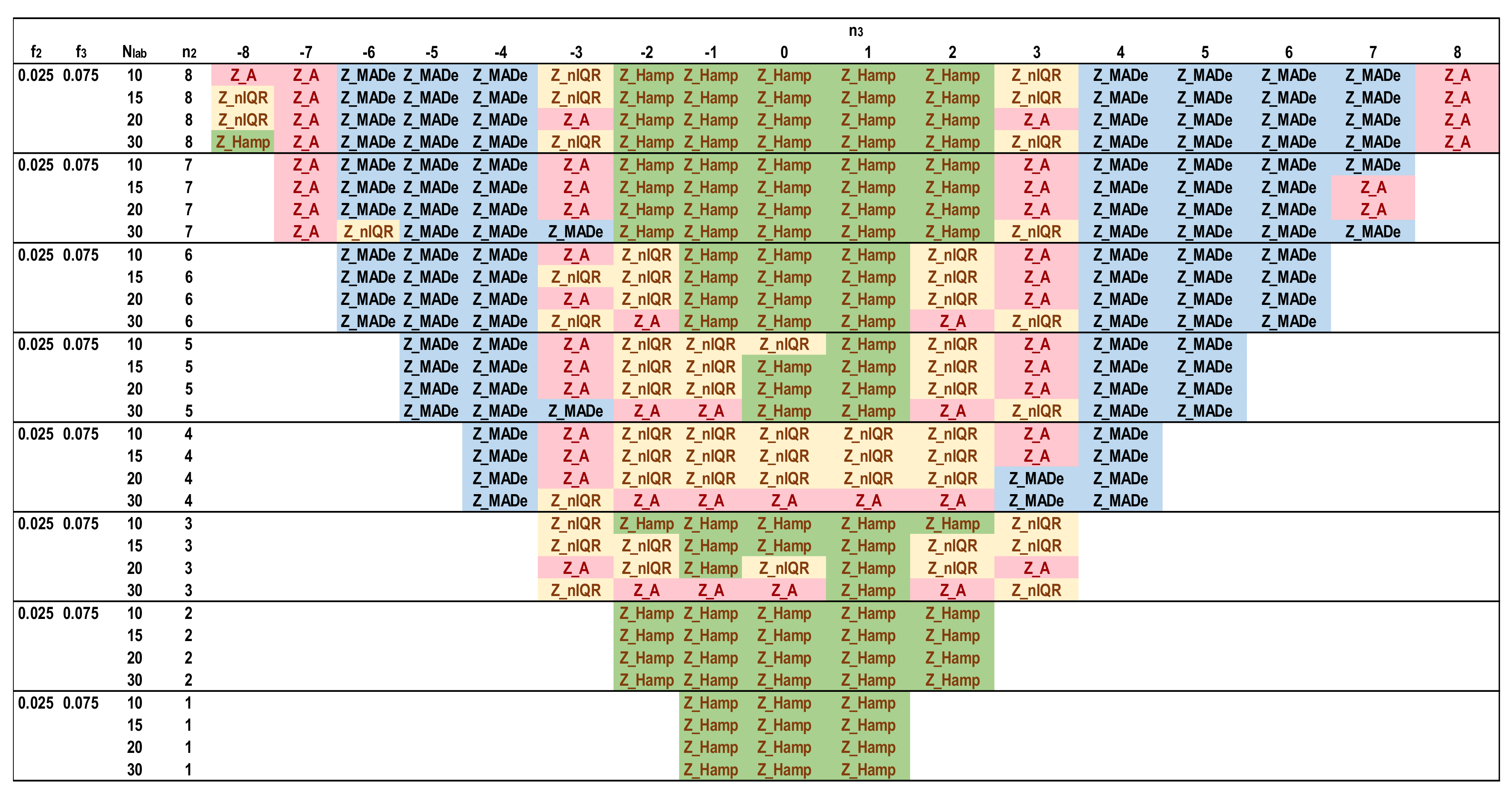
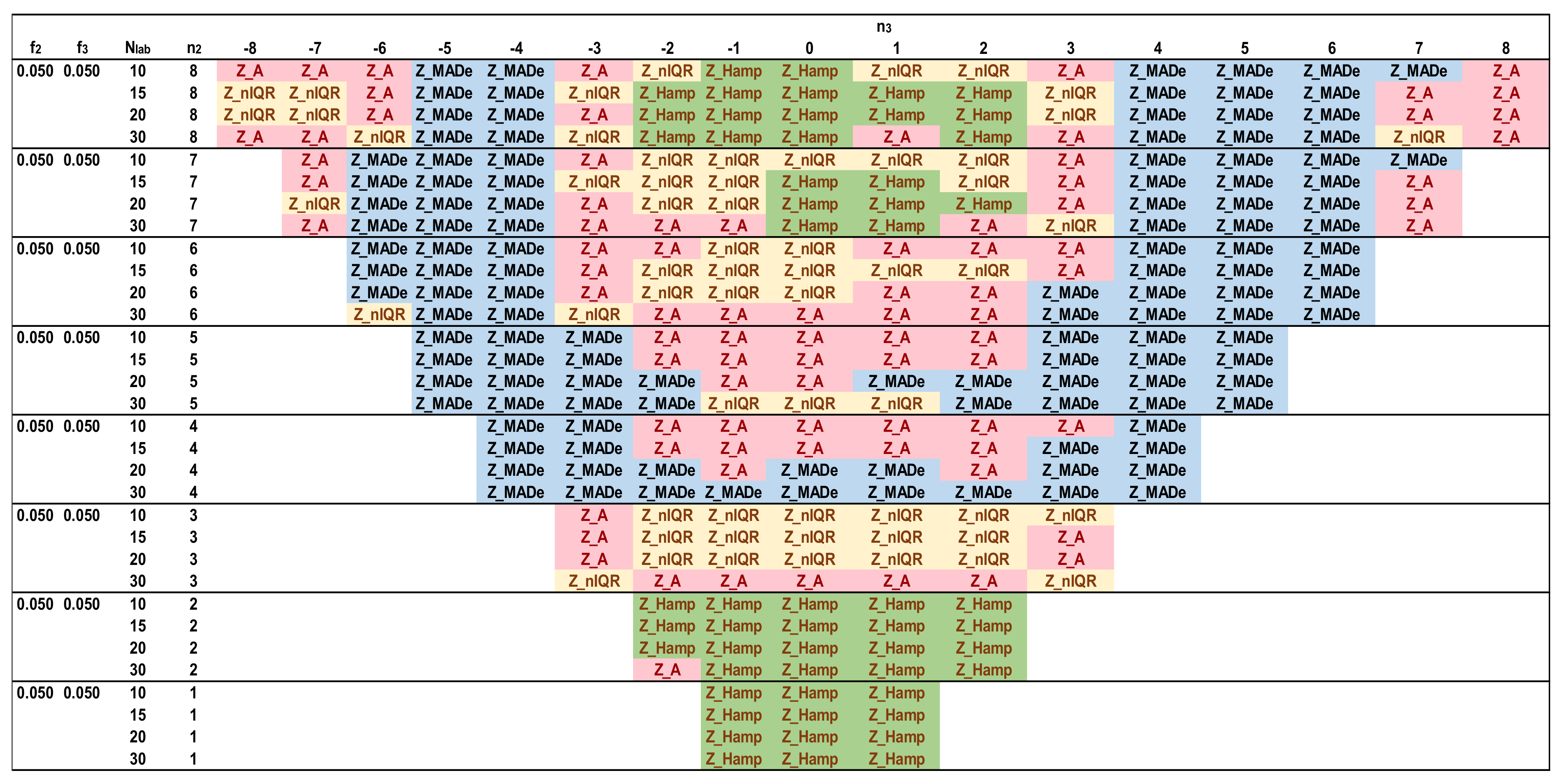
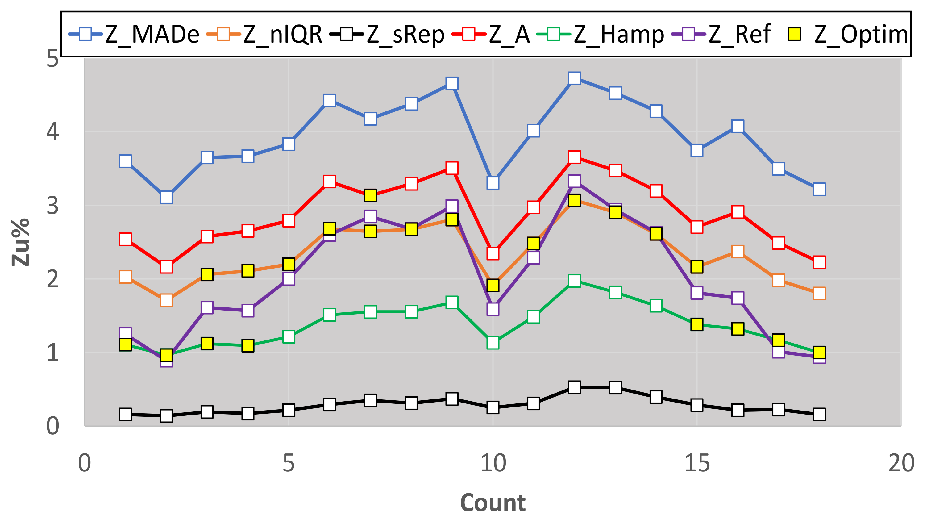
• The best estimator provided by the generalized algorithm depends on the distribution parameters.
• Z_sRep is always much lower than the reference values, Z_Ref, proving that it is not a robust estimator and verifying the findings of Section 3.2.
• For the given levels of N_lab and distribution parameters, Z_MADe is always much higher than Z_Ref and never optimum, verifying paragraph C. 2.3 of 13253:2015 [14] (p. 53). Z_A is closer to Z_Ref than Z_MADe but continuously overestimates Zu%.
• For the given range of m₁, m₂, m₃, and s₁, Z_nIQR and Z_Hamp are the best estimators: the first is 13 times, while the second is 8 times optimal. The results show that Z_Hamp is optimum for lower values of Zu% and Z_nIQR for higher Zu% values.

5. Conclusions

This study developed efficient models in analyzing the results of PT schemes by combining: (a) robust and classical estimators of the population mean and standard deviation; (b) kernel density plots; (c) distributions derived from the addition of two or three Gaussians; (d) Monte Carlo simulations; and (e) Z-factors.

The analysis shows that the sum of two or three normal distributions of adjustable parameters can adequately approximate an actual kernel density plot, so it is a good approximation of the results’ distribution. The one distribution is the main while the others contaminate it. Monte Carlo simulations implemented to such sums of distributions are effective in studying the characteristics of location and dispersion estimators based on ISO 13258:2015 and ISO 5725:2:1994. Assuming a distribution of a large number of results contain Zu% unsatisfactory results according to EN ISO/IEC 17043:2010, the simulator can find the estimators providing non-satisfactory results close to this percentage when the number of labs is limited. The study describes an algorithm solving the above optimization problem with the following constraints: (a) Gaussian, bimodal or trimodal distributions; (b) participants from 10 to 30; (c) fraction of the contaminating population up to 0.10 of the total; (d) variation coefficient of the main distribution equal to 2; (e) equal standard deviations of all the distributions. The analysis proves that using the robust estimators of location and variance is necessary because the classical estimators based on ISO 5725-2:1994 lead to a severe underestimation of the percentage of outliers. The answer to which is the best robust estimator is by no means categoric because the selection depends on the fraction of the contaminating populations and the distances of the mean values of the distributions. The corresponding figures showing the optimal estimators for the constraints (a)–(e) are helpful for a PT expert to decide which estimator to choose if the Gaussian distributions approximating the actual kernel density plot fulfill these constraints. Generally, if the fraction of the contaminating population is ≤0.05 of the total, the selection of MED-MADe is not suitable.

By extending the above, we provided a generalized algorithm, using actual kernel density plots and the previous algorithm, which is not subject to restrictions (b)–(e) and implemented to the results of 18 consecutive rounds of a PT for the 28-day strength of cement with 12–13 participants in average per round. The optimal estimators in the cases studied in this particular test were the MED-nIQR and Q/Hampel methods. The generalized algorithm is suitable for various PT schemes in selecting the optimal robust estimators because it covers an expanded range of the secondary populations’ fractions and unequal standard deviations.

Based on the above arguments, the novelty of this study is the combination of actual kernel density plots and robust estimators through Gaussian distributions and Monte Carlo simulations, helping to select the best robust estimator for the correct calculation of outliers. The investigation of the optimal estimators can continue in the following directions:

▪

The impact of assigned value and standard deviation uncertainty on the Z-factors;

▪

Type I and Type II errors of the estimators;

▪

Comparison of the statistic estimators (a) for a medium and large number of participants; (b) for a range of variation coefficient of results’ distribution;

▪

Direct use of the kernel density plots, by taking into account our generalized algorithm, in determining the best estimator;

▪

Estimators’ comparisons for Z-factors of absolute value between two and three.

References

1. CEN. EN ISO/IEC 17043:2010 Conformity Assessment—General Requirements for Proficiency Testing; CEN Management Centre: Brussels, Belgium, 1994; pp. 2–3, 8–9, 30–33. [Google Scholar]
2. ISO Committee on Conformity Assessment. ISO/IEC 17025:2017 General Requirements for the Competence of Testing and Calibration Laboratories, 3rd ed.; ISO: Geneva, Switzerland, 2017; p. 14. [Google Scholar]
3. Rousseeuw, P.J.; Leroy, A.M. Robust Regression and Outlier Detection; John Wiley & Sons, Inc.: New York, NY, USA, 1987; pp. 9–18. [Google Scholar]
4. Jurečková, J.; Picek, J.; Schindler, M. Robust Statistical Methods with R, 2nd ed.; CRC Press: New York, NY, USA, 2019. [Google Scholar]
5. Wilcox, R.R. Introduction to Robust Estimation and Hypothesis Testing, 5th ed.; Academic Press: London, UK, 2021. [Google Scholar]
6. Hampel, F.R.; Ronchetti, E.M.; Peter, J.; Rousseeuw, P.J.; Stahel, W.A. Robust Statistics: The Approach Based on Influence Functions; John Wiley & Sons, Inc.: New York, NY, USA, 1986. [Google Scholar]
7. Huber, P.J.; Ronchetti, E.M. Robust Statistics, 2nd ed.; John Wiley & Sons, Inc.: Hoboken, NJ, USA, 2009. [Google Scholar]
8. Maronna, R.A.; Martin, R.D.; Yohai, V.J.; Salibián-Barrera, M. Robust Statistics: Theory and Methods (with R), 2nd ed.; John Wiley & Sons, Inc.: Hoboken, NJ, USA, 2018. [Google Scholar]
9. Wang, H.; Mirota, D.; Hager, G.D. A Generalized Kernel Consensus-Based Robust Estimator. IEEE Trans. Pattern Anal. Mach. Intell. 2010, 32, 178–184. [Google Scholar] [CrossRef] [PubMed] [Green Version]
10. Vandermeulen, R.A.; Scott, C.D. Robust Kernel Density Estimation by Scaling and Projection in Hilbert Space. Available online: https://arxiv.org/pdf/1411.4378.pdf (accessed on 16 February 2022).
11. Humbert, P.; Le Bars, B.; Minvielle, L.; Vayatis, N. Robust Kernel Density Estimation with Median-of-Means Principle. Available online: https://arxiv.org/pdf/2006.16590.pdf (accessed on 16 February 2022).
12. Nazir, H.Z.; Schoonhoven, M.; Riaz, M.; Does, R.J. Quality quandaries: A stepwise approach for setting up a robust Shewhart location control chart. Qual. Eng. 2014, 26, 246–252. [Google Scholar] [CrossRef]
13. Nazir, H.Z.; Riaz, M.; Does, R.J. Robust CUSUM control charting for process dispersion. Qual. Reliab. Eng. Int. 2015, 31, 369–379. [Google Scholar] [CrossRef]
14. ISO/TC 69. ISO 13528:2015 Statistical Methods for Use in Proficiency Testing by Interlaboratory Comparison, 2nd ed.; ISO: Geneva, Switzerland, 2015; pp. 12, 32–33, 44–51, 52–62. [Google Scholar]
15. ISO/TC 69. ISO 5725-2:1994 Accuracy (Trueness and Precision) of Measurement Methods and Results—Part 2: Basic Method for the Determination of Repeatability and Reproducibility of a Standard Measurement Method, 1st ed.; ISO: Geneva, Switzerland, 1994; pp. 10–14, 21–22. [Google Scholar]
16. Rousseeuw, P.J.; Croux, C. Alternatives to the Median Absolute Deviation. J. Am. Stat. Assoc. 1993, 88, 1273–1283. [Google Scholar] [CrossRef]
17. Filzmoser, P.; Maronna, R.; Werner, M. Outlier identification in high dimensions. Comput. Stat. Data Anal. 2008, 52, 1694–1711. [Google Scholar] [CrossRef]
18. Kalina, J.; Schlenker, A. A Robust Supervised Variable Selection for Noisy High-Dimensional Data. Biomed. Res. Int. 2015, 320385. [Google Scholar] [CrossRef] [PubMed]
19. Hubert, M.; Debruyne, M.; Rousseeuw, P.J. Minimum covariance determinant and extensions. Wiley Interdiscip. Rev. Comput. Stat. 2018, 10, e1421. [Google Scholar] [CrossRef] [Green Version]
20. Ellison, S.L.R. Applications of Robust Estimators of Covariance in Examination of Inter-Laboratory Study Data. Available online: https://arxiv.org/abs/1810.02467 (accessed on 16 February 2022).
21. Rosário, P.; Martínez, J.L.; Silván, J.M. Evaluation of Proficiency Test Data by Different Statistical Methods Comparison. In Proceedings of the First International Proficiency Testing Conference, Sinaia, Romania, 11–13 October 2007. [Google Scholar]
22. Thompson, M.; Ellison, S.L.R. Fitness for purpose–the integrating theme of the revised harmonized protocol for proficiency testing in analytical chemistry laboratories. Accredit. Qual. Assur. 2006, 11, 467–471. [Google Scholar] [CrossRef]
23. Srnková, J.; Zbíral, J. Comparison of different approaches to the statistical evaluation of proficiency tests. Accredit. Qual. Assur. 2009, 14, 373–378. [Google Scholar] [CrossRef]
24. Tripathy, S.S.; Saxena, R.K.; Gupta, P.K. Comparison of Statistical Methods for Outlier Detection in Proficiency Testing Data on Analysis of Lead in Aqueous Solution. Am. J. Theor. Appl. Stat. 2013, 2, 233–242. [Google Scholar] [CrossRef]
25. Daszykowski, M.; Kaczmarek, K.; Heyden, Y.V.; Walczaka, B. Robust statistics in data analysis—A review: Basic concepts. Chemom. Intell. Lab. Syst. 2007, 85, 203–219. [Google Scholar] [CrossRef]
26. De Oliveira, C.C.; Tiglea, P.; Olivieri, J.C.; Carvalho, M.; Buzzo, M.L.; Sakuma, A.M.; Duran, M.C.; Caruso, M.; Granato, D. Comparison of Different Statistical Approaches Used to Evaluate the Performance of Participants in a Proficiency Testing Program. Available online: https://www.researchgate.net/publication/290293736_Comparison_of_different_statistical_approaches_used_to_evaluate_the_performance_of_participants_in_a_proficiency_testing_program (accessed on 12 February 2022).
27. Kojima, I.; Kakita, K. Comparative Study of Robustness of Statistical Methods for Laboratory Proficiency Testing. Anal. Sci. 2014, 30, 1165–1168. [Google Scholar] [CrossRef] [PubMed] [Green Version]
28. Belli, M.; Ellison, S.; Fajgelj, A.; Kuselman, I.; Sansone, U.; Wegscheider, W. Implementation of proficiency testing schemes for a limited number of participants. Accredit. Qual. Assur. 2007, 12, 391–398. Available online: https://link.springer.com/article/10.1007/s00769-006-0247-0 (accessed on 16 February 2022). [CrossRef] [Green Version]
29. Kuselman, I.; Belli, M.; Ellison, S.L.R.; Fajgelj, A.; Sansone, U.; Wegscheider, W. Comparability and compatibility of proficiency testing results in schemes with a limited number of participants. Accredit. Qual. Assur. 2007, 12, 563–567. Available online: https://link.springer.com/article/10.1007/s00769-007-0309-y (accessed on 16 February 2022). [CrossRef]
30. Hund, E.; Massart, D.; Smeyers-Verbeke, J. Inter-laboratory studies in analytical chemistry. Anal. Chim. Acta 2000, 423, 145–165. [Google Scholar] [CrossRef]
31. Working Group 1 of the Joint Committee for Guides in Metrology. ISO/IEC GUIDE 98-3/Suppl.1 Uncertainty of Measurement, Part 3: Guide to the Expression of Uncertainty in Measurement (GUM:1995), Supplement 1: Propagation of Distributions Using a Monte Carlo Method; ISO: Geneva, Switzerland, 2008. [Google Scholar]
32. CEN/TC 51. EN 196-1:2005, Methods of Testing Cement–Part 1: Determination of Strength; CEN Management Centre: Brussels, Belgium, 2005. [Google Scholar]
33. CEN/TC 51. EN 197-1:2011, Cement. Part 1: Composition, Specifications and Conformity Criteria for Common Cements; Management Centre: Brussels, Belgium, 2011. [Google Scholar]
34. Simpson, D.G.; Yohai, V.J. Functional stability of one-step GM-estimators in approximately linear regression. Ann. Statist. 1998, 26, 1147–1169. [Google Scholar] [CrossRef]
35. Cochran Variance Outlier Test. Available online: https://www.itl.nist.gov/div898/software/dataplot/refman1/auxillar/cochvari.htm (accessed on 5 January 2022).
36. Grubbs’ Test for Outliers. Available online: https://www.itl.nist.gov/div898/handbook/eda/section3/eda35h1.htm (accessed on 5 January 2022).
Figure 1. Examples of kernel density plots.
Computation 10 00044 g001
Figure 2. Actual distributions, kernel plots, and calculated distributions for all the yearly results.
Computation 10 00044 g002
Figure 3. Distribution of populations consisting of a main and secondary distribution. Dashed lines; main and secondary groups, and solid line; total population.
Computation 10 00044 g003
Figure 4. Distribution of populations consisting of a main and two secondary distribution. Dashed lines; main and secondary groups, and solid line; total population.
Computation 10 00044 g004
Figure 5. Average values of the population standard deviations. MADe: scaled median absolute deviation; nIQR: normalized interquartile range; sRep: reproducibility standard deviation without outliers; As*: standard deviation—Algorithm A; Hs*, 0.40: standard deviation using Q method and sr = 0.40; Hs*, 0.01: standard deviation using the Q method and sr = 0.01.
Computation 10 00044 g005
Figure 6. Standard deviations of the population standard deviations. MADe: scaled median absolute deviation; nIQR: normalized interquartile range; sRep: reproducibility standard deviation without outliers; As*: standard deviation—Algorithm A; Hs*, 0.40: standard deviation using Q method and sr = 0.40; Hs*, 0.01: standard deviation using Q method and sr = 0.01.
Computation 10 00044 g006
Figure 7. Distribution of the population standard deviations.
Computation 10 00044 g007
Figure 8. Function between Zu% and number of standard deviations n2, n3, and Nlab = 400. Calculation of initial values using step (iv) of Section 3.2.
Computation 10 00044 g008
Figure 9. Functions between Zu% and number of standard deviations n2, for the reference values and robust estimators, and Nlab = 10, 15, 20, 30.
Computation 10 00044 g009
Figure 10. Functions between Zu% and number of standard deviations n3, for the reference values and robust estimators, and Nlab = 10, 15, 20, 30.
Computation 10 00044 g010
Figure 11. Optimal robust estimators of Zu% for number of standard deviations n2 = 0 to 8, f2 = 0.025 to 0.10 and Nlab = 10, 15, 20, 30.
Computation 10 00044 g011
Figure 12. Optimal robust estimators of Zu% for trimodal distributions, f2 = 0.025 and f3 = 0.025.
Computation 10 00044 g012
Figure 13. Optimal robust estimators of Zu% for trimodal distributions, f2 = 0.025 and f3 = 0.05.
Computation 10 00044 g013
Figure 14. Optimal robust estimators of Zu% for trimodal distributions, f2 = 0.025 and f3 = 0.075.
Computation 10 00044 g014
Figure 15. Optimal robust estimators of Zu% for trimodal distributions, f2 = 0.05 and f3 = 0.05.
Computation 10 00044 g015
Figure 16. Estimators of Zu% for 18 rounds of the 28-day strength test.
Computation 10 00044 g016