Mathematical Modeling: Global Stability Analysis of Super Spreading Transmission of Respiratory Syncytial Virus (RSV) Disease

Abstract

In this paper, a model for the transmission of respiratory syncytial virus (RSV) in a constant human population in which there exist super spreading infected individuals (who infect many people during a single encounter) is considered. It has been observed in the epidemiological data for the diseases caused by this virus that there are cases where some individuals are super-spreaders of the virus. We formulate a simply SEI_rI_sR (susceptible–exposed–regular infected–super-spreading infected–recovered) mathematical model to describe the dynamics of the transmission of this disease. The proposed model is analyzed using the standard stability method by using Routh-Hurwitz criteria. We obtain the basic reproductive number ($R_0$) using the next generation method. We establish that when $R_0<1$, the disease-free state is locally asymptotically stable and the disease endemic state is unstable. The reverse is true when $R_0>1$, the disease endemic state becomes the locally asymptotically stable state and the disease-free state becomes unstable. It is also established that the two equilibrium states are globally asymptotically stable. The numerical simulations show how the dynamics of the disease change as values of the parameters in the SEI_rI_sR are varied.

1. Introduction

Respiratory syncytial virus (RSV) (a single-stranded RNA virus) is a common respiratory virus. RSV causes respiratory tract diseases such as infection of the airway, of the lungs, and of the middle ear. It is the most common cause of the common cold, Bronchitis, Croup, Bronchiolitis, and of Pneumonia. This virus usually causes severe infection in some people, especially in premature babies, older adults, infants, and adults with heart and lung disease, and in anyone who has a very weak immune system [1,2,3,4,5,6]. The virus can be transmitted by direct contact with infectious secretions or be spread by droplets from the cough of infected people. It can be accidentally transmitted by contact with hands that have been contaminated by touching eating utensils or any articles that have been freshly soiled by nasal or throat discharges of an infected person. In other words, the virus is easily spread. The incubation period is 1–10 days, usually 5–7 days. The infection usually subsides in about 1–2 weeks. Most cases are mild and the patients can be managed with standard treatment. Severe cases may however need oxygen therapy and tube feeding [1,2,3,4,7,8]. Antiviral agents should be considered for patients with congenital heart or lung diseases. Antibiotics may be needed only if there are bacterial complications such as pneumonia, sinusitis, or otitis media. Respiratory disease causes an immense worldwide health burden. It is estimated that 235 million people suffer from asthma, more than 200 million people have chronic obstructive pulmonary disease (COPD), 65 million moderate-to-severe COPD, 1–6% of the adult population (more than 100 million people) experience tumultuous millions with pulmonary hypertension, and more than 50 million people struggle with occupational lung diseases. In total, more than 1 billion persons suffer from chronic respiratory conditions. It is estimated that illnesses associated with RSV infections cause about 24.8 million cases and 76,600 deaths annually [1,2,3,4,9,10,11,12].

This study aims to systematically aggregate and analyze the published epidemiological data regarding respiratory tract infections. The published data for some of the diseases caused by some of the respiratory syncytial virus indicate the existence of super-spreaders of the diseases, i.e., individuals who infect many other people, not just one or two. These were first seen at the start of the SARS (severe acute respiratory syndrome) epidemic where a single medical doctor infected the 11 other people on an elevator in Hong Kong in 2003 [12]. This type of individual was again seen during the Middle East Respiratory Syndrome (MERS) epidemic in Korea in 2016 and in patients with acute Middle East syndrome coronavirus (MERS-CoV) pneumonia in 2018 [13,14,15]. In both cases, the illnesses were caused by the corona-virus. In the present pandemic which is caused by the COVID-19 virus, situations where many individuals are infected are referred to as a superinfection event. At these events, a person with a high viral load would have been present. We will refer to this type of infected person as I_s, a person having a high viral load. When this person coughs, a large amount of the corona virus is introduced into the environment. We adopt a SEI_rI_sR (susceptible–exposed–regular infected–super-spreading infected–recovered) model for two infection groups in this model, where the transmission rate in humans will be one of the control factors [10,16,17,18]. A study of the possible behaviors simulated by numerically solving the mathematical models as the values of the parameters used in the model are varied will allow to control the epidemic caused by Respiratory syncytial virus (RSV).

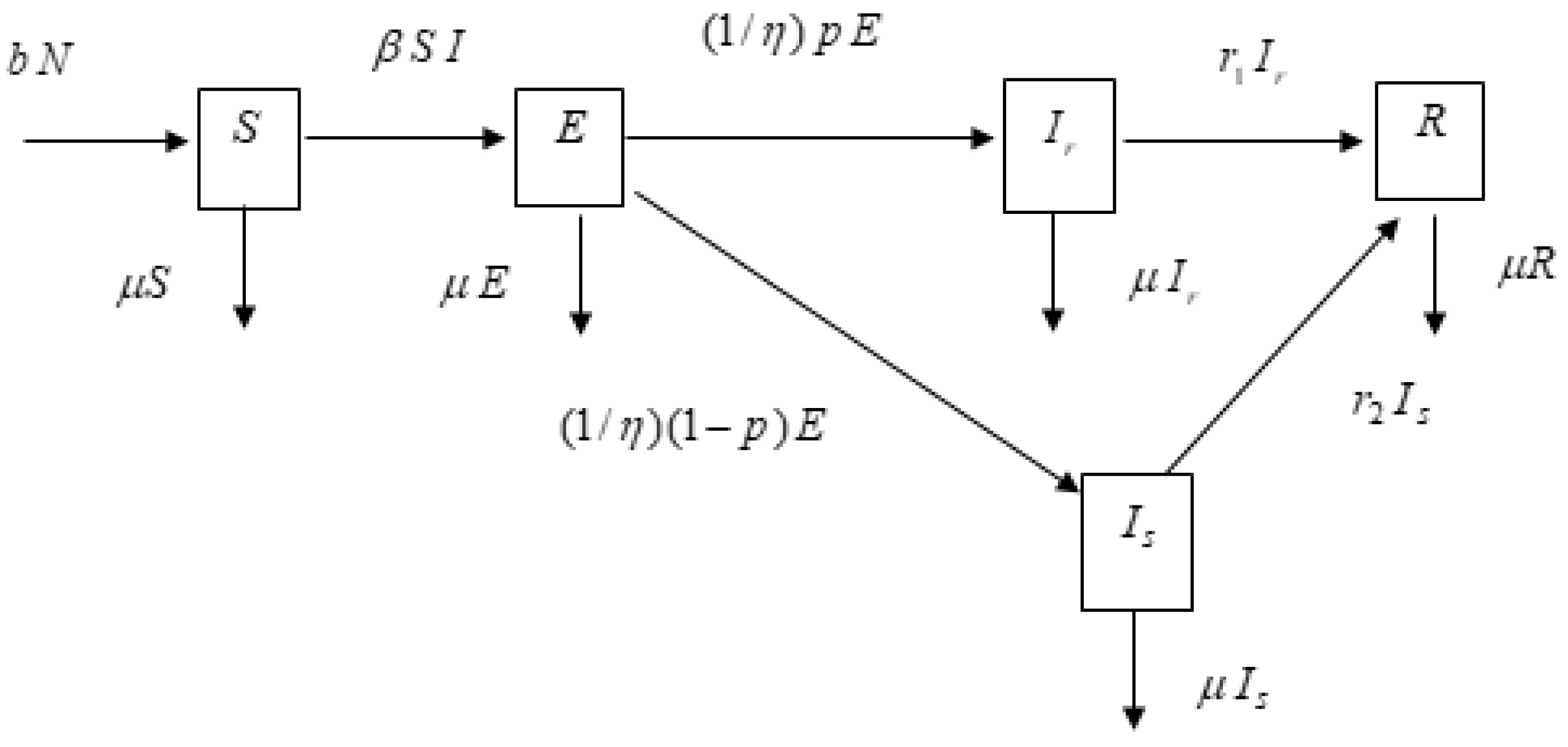
2. Materials and Methods

Based on the epidemic SIR (susceptible–infected–recovered) model implemented by Youngmin Kim and Namsuk Cho [18,19,20,21,22,23,24] and Zhen Jin and Pongsumpun et al. [13,14,15,24], we have developed this SIR model by adding exposed individuals (E) as well as two classes of infected individuals (I_r and I_s) to create the SEI_rI_sR model. The respiratory syncytial virus may die or multiply into a normal amount or high amount of new RSV’s in the person depending on the immunological status of the individual. This means that the exposed person can become a R, I_r, or I_s. What occurs to a particular exposed individual can only be determined after it happens. Taking into account what we have just mentioned, we propose the following SEIR model to describe the dynamics of four sub population (classes): susceptible, exposed, normal infectious, super infectious, and recovered individuals, whose flow charts are shown on Figure 1.

From the above flow chart, we see that the transmission dynamics of the respiratory disease are given by the following set of ordinary differential equations, which are just the mathematical expressions of the time rate of changes in the number of individuals of each class being equal to the number entering into the class minus the number leaving:

$$\frac{dS(t)}{dt} = bN - \beta S(t) I(t) - \mu S(t)$$

(1)

$$\frac{dE(t)}{dt} = \beta S(t) I(t) - \left(\frac{1}{\eta }\right)p E(t) - \left(\frac{1}{\eta }\right)( 1 - p) E (t) - \mu E(t)$$

(2)

$$\frac{d{I}_r(t)}{dt} = \left(\frac{1}{\eta }\right)pE (t) - r_1{I}_r(t) - \mu I_r (t)$$

(3)

$$\frac{d{I}_s(t)}{dt} = \left(\frac{1}{\eta }\right)( 1 - p) E(t) - r_2{I}_s (t) - \mu I_s (t)$$

(4)

$$\frac{dR(t)}{dt} = r_1{I}_r(t) + r_2{I}_s(t) - \mu R(t)$$

(5)

where

$b$ is the birth rate of the human population;

$N$ is the total human population;

$\mu$ is the death rate of human population;

$\beta$ is the transmission rate of virus between human;

$\eta$ is the incubation time of virus in human;

$p$ is the probability that a new case will be a normal infected human;

$(1-p)$ is the probability that a new case will be a super-spreading infected human;

$r_1$ is the recovery rate of regular infected human;

$r_2$ is the recovery rate of super-spreading infected human.

Proposition 1.

Let $(S^{\prime }(t), E^{\prime }(t), I_r{}^{\prime }(t), I_s{}^{\prime }(t), R^{\prime }(t))$ be the solutions of Equations (1)–(5). Denoting also the invariant set $\psi = \{(S^{\prime }(t), E^{\prime }(t), {I^{\prime }}_r(t), {I^{\prime }}_s(t), R^{\prime }(t) ) \in R_{+}^5 : N \le \frac{b}{\mu }\}$. Then the closed set $\psi$ is positive invariant.

Proof of Proposition 1.

We set $N (t) = (S^{\prime }(t)+ E^{\prime }(t)+ {I^{\prime }}_r(t)+ {I^{\prime }}_s(t)+ R^{\prime }(t))$ and assume that $N \le \frac{b}{\mu }$. Note that the total population $N$ is non–negative on $R_{+}^5$. Then we have:

$$\begin{array}{ll}\frac{dN(t)}{dt}& =\frac{dS(t)}{dt}+\frac{dE(t)}{dt}+\frac{d{I}_r(t)}{dt}+\frac{d{I}_s(t)}{dt}+\frac{dR(t)}{dt}\\ & =(bN-\beta S(t)I(t)-\mu S(t))+(\beta S(t)I(t)-\left(\frac{1}{\eta }\right)pE(t)-\left(\frac{1}{\eta }\right)(1-p)E(t)-\mu E(t))\\ & +(\left(\frac{1}{\eta }\right)pE(t)-r_1{I}_r(t)-\mu I_r(t))+(\left(\frac{1}{\eta }\right)(1-p)E(t)-r_2{I}_s(t)-\mu I_s(t))+\\ & (r_1{I}_r(t)+r_2{I}_s(t)-\mu R(t))\\ & =bN-\mu (S(t)+E(t)+I_r(t)+I_s(t)+R(t))\le b-\mu N\end{array}$$

Then it follows that $\frac{dN}{dt} \le 0$ on $0 \le N (t) \le N(0)e^{-\mu t} + \frac{b}{\mu } (1 - e^{\mu t})$. As $t \to \infty , e^{-\mu t} \to \infty$ and we have $\underset{t\to \infty }{\lim } N (t) \le \frac{b}{\mu }, N(t)$ approaches $\frac{b}{\mu }$. Since the region of all solutions of Ψ is in $R_{+}^5$ [8,10,12]. □

3. Analysis of the Model

3.1. Equilibrium Points

For this model, there are two equilibrium points: the disease-free equilibrium point and an endemic equilibrium point. Two equilibrium points are found by setting the right hand side (RHS) of Equations (1)–(5) to zero [19].

Proposition 2.

The equilibrium point is the disease-free steady state ${\mathit{\zeta }}_1^{*} = (S^{*}(t),E^{*}(t),I_r^{*}(t), I_s^{*}(t),R^{*}(t)) \in \psi$ for $R_0 \le 1$. For $R_0 > 1$, the equilibrium point is the endemic steady state ${\mathit{\zeta }}_2^{*} = (S^{*}(t),E^{*}(t),I_r^{*}(t), I_s^{*}(t),R^{*}(t)) \in \psi$ and we will $E^{*}\left(t\right)\ne 0, I_r^{*}\left(t\right)\ne 0$ and $I_s^{*}\left(t\right)\ne 0$ Performing the steps of setting the RHS of Equations (1)–(5) to zero,[17,18,19,20,21,22]we get

A. Disease-free equilibrium points${\zeta }_1^{*}=(S^{*}(t),E^{*}(t),I_r^{*}(t),I_s^{*}(t),R^{*}(t))\in \psi$

$${\zeta }_1^{*} = (\frac{bN}{\mu }, 0 , 0, 0 , 0 )$$

B. Endemic Equilibrium Points ${\zeta }_2^{*}=(S^{*}(t),E^{*}(t),I_r^{*}(t),I_s^{*}(t),R^{*}(t))\in \psi ,$ we obtained

$$S^{*}(t) = ( 1 + \mu \eta ) A C$$

$$E^{*}(t) = \eta (- \mu C A + B)$$

$$I_r{}^{*} (t) = \frac{p (- B + \mu A C ) }{r_1 + \mu }$$

$$I_s{}^{*}(t) = \frac{ B ( - 1+ p ) (-1 + \mu A C ) }{r_2 + \mu }$$

$$R^{*}(t) = \frac{(-B + \mu A C ) ( - (- 1 + p) r_2 \mu + r_{1 }(r_{2 }+ p\mu )}{\mu C}$$

where

$$A=\frac{1}{\beta (r_1 - p r_1 +p r_2 + \mu ) },B=\frac{bN}{1 + \eta },C=(r_1+\mu )(r_2+\mu )$$

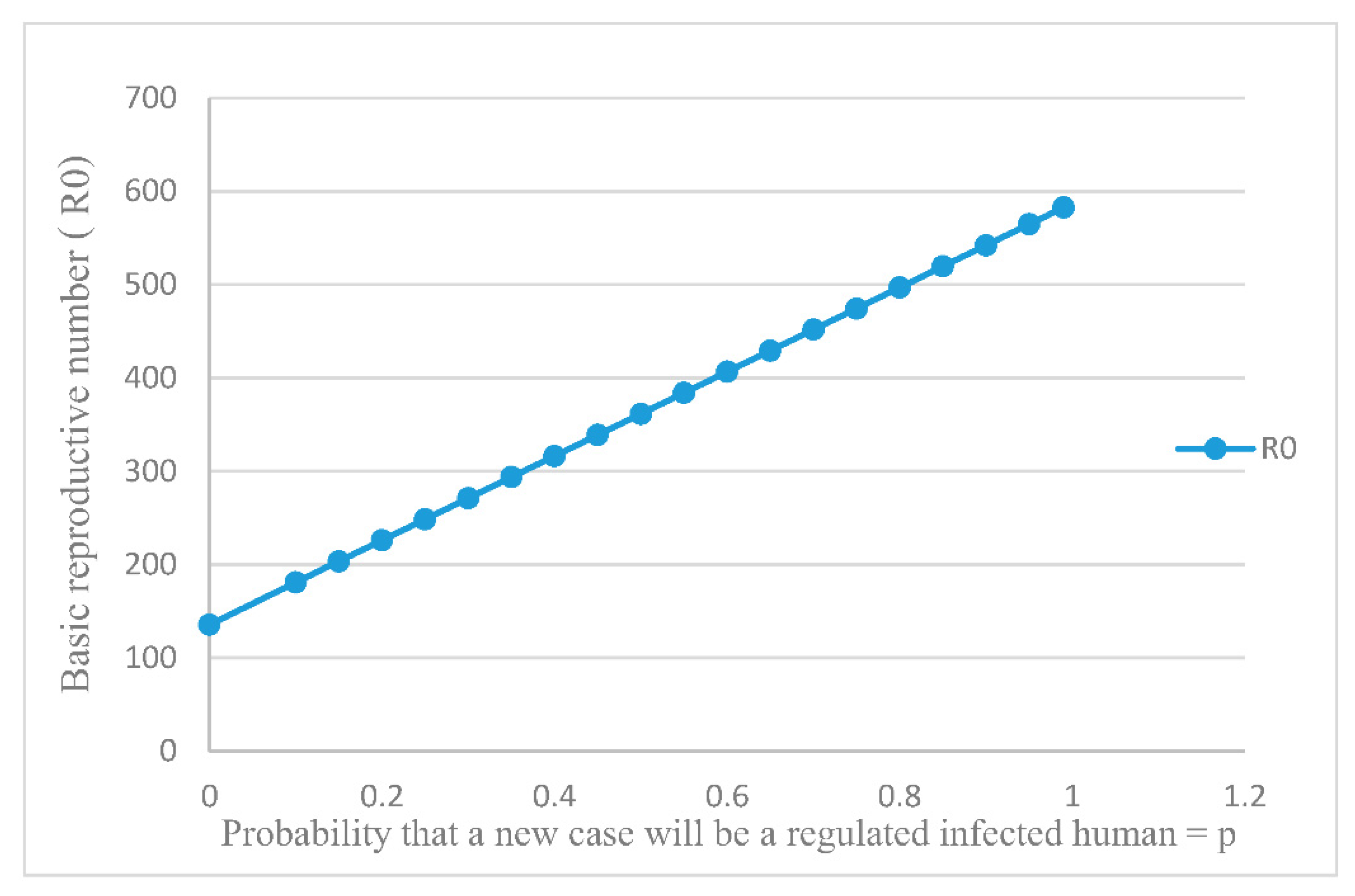
3.2. Basic Reproductive Number

The basic reproductive number ($R_0$) is an important threshold in mathematical epidemiology. It can be obtained by the next generation method and is the spectral radius (Van den Driessche and Watmough, 2002) [19,20,21]. We now rewrite the equations in the matrix from

$$\frac{dX}{dt} = F(x) - V(x)$$

where,$F(x)$ is the matrix of new infectious and $V(x)$ is the matrix for the transfers between the compartments in the infective equations. Doing this, we have;

$$X = \left[\begin{array}{c}S(t)\\ E(t)\\ I_r(t)\\ I_s(t)\\ R(t)\end{array}\right] , F(x) = \left[\begin{array}{c}0\\ \beta S(t) I(t) \\ 0\\ 0\\ 0\end{array}\right] \mathrm{and}$$

$$V(x) = \left[\begin{array}{c} -bN + \beta S(t) I(t) + \mu S (t) \\ \left(\frac{1}{\eta }\right)p E(t) + \left(\frac{1}{\eta }\right) ( 1 - p) E(t) + \mu E (t) \\ -\left(\frac{1}{\eta }\right)p E(t) + r_1{I}_r(t) + \mu I_r(t) \\ -\left(\frac{1}{\eta }\right)E (t)- \left(\frac{1}{\eta }\right) pE(t) + r_2{I}_s(t) + \mu I_s(t)\\ -r_1{I}_r(t) - r_2{I}_s (t) + \mu R(t) \end{array}\right]$$

We now evaluate the Jacobian of $F(x)$ and $V(x)$ at the first equilibrium point ${\zeta }_1^{*} = (\frac{b}{\mu }, 0 , 0, 0 , 0 )$, and put them into the form $DF (x) = F$ and $DV (x) = V$.

We now define $R_0$ as the threshold for the stability of the disease-free equilibrium ${\zeta }_1^{*}$. It will now have the matrix form

$$R_0 = \rho (F{V}^{-1})$$

where $\rho$ is defined as the spectral radius of the next generation matrix FV⁻¹. For our model, the Jacobian matrix [21] becomes

$$F({\zeta }_1) = \left[\begin{array}{ccccc}0& 0& 0& 0& 0\\ \beta I(t) & 0 & \beta S(t)& \beta S(t)& 0\\ 0& 0& 0& 0& 0\\ 0& 0& 0& 0& 0\\ 0& 0& 0& 0& 0\end{array}\right]$$

and

$$V({\zeta }_1) = \left[\begin{array}{ccccc} \beta I + \mu & 0& \beta S(t)& \beta S(t)& 0\\ 0& \left(\frac{1}{\eta }\right)p + \left(\frac{1}{\eta }\right) ( 1 - p) + \mu & 0& 0& 0\\ 0& -\left(\frac{1}{\eta }\right)p& r_1 + \mu & 0& 0\\ 0& -\left(\frac{1}{\eta }\right) - \left(\frac{1}{\eta }\right) p& 0& r_2 + \mu & 0\\ 0& 0& -r_1& -r_2& \mu \end{array}\right]$$

Therefore, the next generation matrix is given as follows:

$$F{V}^{-1} = \left[\begin{array}{ccccc}0& 0& -\frac{b^2{\beta }^2(r_1+p{r}_1+p{r}_2+\mu +2p\mu )}{{\mu }^3(r_1 +\mu )(r_2+\mu )(1+\mu \eta )}& -\frac{b^2{\beta }^2(r_1+p{r}_1+p{r}_2+\mu +2p\mu )}{{\mu }^3(r_1 +\mu )(r_2+\mu )(1+\mu \eta )}& 0\\ 0& 0& \frac{b\beta \eta }{\mu +{\mu }^2\eta }& \frac{b\beta \eta }{\mu +{\mu }^2\eta }& 0\\ 0& 0& \frac{b p\beta }{\mu (r_1 +\mu )(1+\mu \eta )}& \frac{b p\beta }{\mu (r_1 +\mu )(1+\mu \eta )}& 0\\ 0& 0& \frac{b(1+p)\beta }{\mu (r_2+\mu )(1+\mu \eta )}& \frac{b(1+p)\beta }{\mu (r_2+\mu )(1+\mu \eta )}& 0\\ 0& 0& \frac{b\beta ((1+p)r_2 \mu + r_1(r_2 + 2p{r}_2+p\mu ))}{{\mu }^2(r_1+\mu ) (r_2+\mu )(1+\mu \eta )}& \frac{b\beta ((1+p)r_2 \mu + r_1(r_2 + 2p{r}_2+p\mu ))}{{\mu }^2(r_1+\mu ) (r_2+\mu )(1+\mu \eta )}& 0\end{array}\right]$$

The spectral radius of $F{V}^{-1}$ is given as $\rho (F{V}^{-1})$

$$\rho (F{V}^{-1}) = \left[\begin{array}{ccccc}-\lambda & 0& -\frac{b^2{\beta }^2(r_1+p{r}_1+p{r}_2+\mu +2p\mu )}{{\mu }^3(r_1 +\mu )(r_2+\mu )(1+\mu \eta )}& -\frac{b^2{\beta }^2(r_1+p{r}_1+p{r}_2+\mu +2p\mu )}{{\mu }^3(r_1 +\mu )(r_2+\mu )(1+\mu \eta )}& 0\\ 0& -\lambda & \frac{b\beta \eta }{\mu +{\mu }^2\eta }& \frac{b\beta \eta }{\mu +{\mu }^2\eta }& 0\\ 0& 0& \left(\frac{b p\beta }{\mu (r_1 +\mu )(1+\mu \eta )}\right)-\lambda & \frac{b p\beta }{\mu (r_1 +\mu )(1+\mu \eta )}& 0\\ 0& 0& \frac{b(1+p)\beta }{\mu (r_2+\mu )(1+\mu \eta )}& \left(\frac{b(1+p)\beta }{\mu (r_2+\mu )(1+\mu \eta )}\right)-\lambda & 0\\ 0& 0& \frac{b\beta ((1+p)r_2 \mu + r_1(r_2 + 2p{r}_2+p\mu ))}{{\mu }^2(r_1+\mu ) (r_2+\mu )(1+\mu \eta )}& \frac{b\beta ((1+p)r_2 \mu + r_1(r_2 + 2p{r}_2+p\mu ))}{{\mu }^2(r_1+\mu ) (r_2+\mu )(1+\mu \eta )}& -\lambda \end{array}\right]$$

where

$$\rho (F{V}^{-1}) = \mu (r_1 +\mu )(r_2+\mu )(1+\mu \eta )$$

We obtain

$$R_0 = \frac{b \beta (r_1+ p r_1 + p{r}_2 + \mu +2 p\mu )}{\mu (r_1 +\mu ) (r_2+\mu ) (1+\mu \eta )}$$

(6)

As it appears in (6), the basic reproductive number of systems defined by Equations (1)–(5) depends on the parameter appearing in the system of equations.

3.3. Local Asymptotical Stability

Theorem 1.

(i) The disease-free steady state is locally asymptotically stable if.

Proof of Theorem 1.

We apply the Routh–Hurwitz criterion. First, we calculate the Jacobian matrix at the disease-free steady state and obtain

$$J_0 = \left[\begin{array}{cccc}(- \mu )- \lambda & 0& - \beta (\frac{b}{\mu })& - \beta (\frac{b}{\mu }) \\ 0 & (- \left(\frac{1}{\eta }\right)p - \left(\frac{1}{\eta }\right) ( 1 - p) - \mu )- \lambda & \beta (\frac{b}{\mu }) & \beta (\frac{b}{\mu }) \\ 0& \left(\frac{1}{\eta }\right)p & ( - r_1- \mu )- \lambda & 0\\ 0& \left(\frac{1}{\eta }\right) ( 1 - p) & 0& (- r_2 - \mu )- \lambda \end{array}\right] = 0$$

(7)

The eigenvalues of the $J_0$ are obtained by solving det(J₀ − λI = 0). We obtained the characteristic Equation (7):

$$(\lambda +\mu )({\lambda }^3+a_1{\lambda }^2+a_2\lambda +a_3)=0$$

where:

$$a_1=\frac{\mu + r_1 \mu \eta +r_2 \mu \eta +3 {\mu }^3 \eta }{\mu \eta }$$

$$a_2=\frac{1}{\mu \eta }(-b\beta +\mu (r_1+r_2+2\mu +(r_1{r}_2+2(r_1+r_2)\mu +3{\mu }^3)\eta ))$$

$$a_3 = \frac{1}{\mu \eta }(b\beta ((-1 + p ) r_1 - p{r}_2 - \mu ) + \mu (r_1+\mu ) (r_2 +\mu ) (1+ \mu \eta )$$

Under the assumption$b > \mu$, that the birth rate is greater than the death rate. According to the Routh–Hurwitz criterion [10,16,25], the following three conditions have to be satisfied: [16,19]

$$a_{1 }>0, a_3>0, a_1{a}_2>a_3$$

It is seen that $a_{1 }>0$ if $R_0<1.$This is the case for the second condition that $a_3>0.$For the last condition, we have

$$a_{1 }{a}_2 = \frac{1}{\mu {\eta }^2} (1 + (r_1 + r_2 + 3\mu )\eta (-b\beta + \mu (r_1 + r_2 + 2\mu +(r r_2 +2(r_1 + r_2) \mu +3{\mu }^3)\eta )).$$

We can see that $a_1{a}_2>a_3$ for $R_0<1$, and so based on the Routh–Hurwitz criterion, the disease-free steady state is locally asymptotically stable if and only if $R_0 < 1$.

(ii) The disease endemic steady state is locally asymptotically stable if $R_0\ge 1$. At the disease endemic equilibrium point ${\zeta }_2^{*}=(S^{*},E^{*},I_r^{*},I_s^{*},R^{*})$the Jacobian is given by

$$J_1 = \left[\begin{array}{cccc}(- \beta ( I_r{}^{*} +I_s{}^{*}) - \mu )- \lambda & 0& - \beta S^{*}& - \beta S^{*} \\ \beta S ( I_r{}^{*} +I_s{}^{*}) & (- \left(\frac{1}{\eta }\right)p - \left(\frac{1}{\eta }\right) ( 1 - p) - \mu )- \lambda & \beta S^{*} & \beta S^{*} \\ 0& \left(\frac{1}{\eta }\right)p & ( - r_1- \mu )- \lambda & 0\\ 0& \left(\frac{1}{\eta }\right) ( 1 - p) & 0& (- r_2 - \mu )- \lambda \end{array}\right] = 0.$$

The characteristic equation of the above matrix is

$${\lambda }^4 + c_1{\lambda }^3 + c_2{\lambda }^2 + c_3{\lambda }^{} + c_4 = 0$$

where

$$c_1 = (I_r{}^{*}(t) + I_s{}^{*}(t))\beta + r_1 + r_2 +4\mu + \frac{1}{\eta }$$

$$\begin{array}{l}{c}_2 = \left(\frac{1}{\eta }\right) (((I_r{}^{*}(t) + I_s{}^{*}(t)- S^{*}(t))\beta + r_1 + r_2 +3\mu + ( r_1{r}_2 + 3 (r_1 + r_2 )\mu + 6{\mu }^2 + I_r{}^{*}(t) \beta ( r_1 + r_2 +3\mu ) +\\ I_s{}^{*}(t)\beta ( r_1 + r_2 +3\mu ) )\eta )\end{array}$$

$$\begin{array}{l}{c}_3 = \left(\frac{1}{\eta }\right)(-S^{*}(t)\beta r_1 + p S^{*(t)}\beta r_1 - p S^{*}(t)\beta r_2 +r_1 r_2 - 2 S^{*}(t)\beta \mu + 2r_1 \mu + 2 r_2 \mu + 3{\mu }^3 + \\ \mu ( 2r_1 r_2 + 3 (r_1 + r_2 ) \mu + 4 {\mu }^2 ) \eta + I_r{}^{*}(t) \beta ( r_1 + r_2 +2\mu + (r_1 r_2 + 2 (r_1 + r_2 ) \\ \mu + 3{\mu }^2 )\eta )+I_s{}^{*}(t)\beta (r_1 + r_2 + 2\mu + (r_1 r_2 + 2 (r_1 + r_2 ) \mu + 3{\mu }^2)\eta )) \end{array}$$

$$\begin{array}{l}{c}_4 = \left(\frac{1}{\eta }\right) (I_r{}^{*}(t)\beta (r_1 + \mu ) ( r_2 + \mu ) (1+ \mu \eta ) + I_s{}^{*}(t)\beta (r_1 + \mu ) ( r_2 + \mu ) (1+ \mu \eta ) \\ + \mu (S^{*} (t)\beta ((-1 + p) r_1 - p r_2 - \mu ) + (r_1 + \mu ) ( r_2 + \mu ) (1+ \mu \eta ) ))\end{array}$$

The four eigenvalues of ${\lambda }^4+c_1{\lambda }^3+c_2{\lambda }^2+c_3{\lambda }^{}+c_4=0$ will have a negative real part if they satisfy the Routh–Hurwitz criteria. Thus, ${\zeta }_2^{*}$ will be locally asymptotically stable for $R_0\ge 1$ if the following conditions are satisfied:

$$c_1 > 0, c_3 > 0, c_4 > 0, c_1{c}_2{c}_3 > {c_3}^2+{c_1}^2{c}_4$$

It can be easily seen that the four conditions are satisfied and so the endemic equilibrium state${\zeta }_2^{*} = (S^{*}(t),E^{*}(t),I_r^{*}(t), I_s^{*}(t),R^{*}(t)) \in \psi$is locally asymptotically stable when$R_0 > 1$.

Proposition 3.

Let $(S(t), E(t), I_r(t), I_s(t), R(t))$ be the solution of (1)–(5) with the initial condition $(S(0), E(0), I_r(0), I_s(0), R(0))$ and the compact set

$$\psi = \left\{(S(t), E(t), I_r(t), I_S(t), R(t)) \in R_5^{+}, P \le N_T = \frac{b}{\mu }\right\}$$

is a positively invariant set that attracts all solutions in $R_5^{+}$.

Proof of Proposition 3.

We define the Lyapunov function as

$P\left(t\right)=\left(P_1\right(t\left)\right)$$= ( S(t) + E(t) + I_r(t) + I_s(t) + R (t))$ being positive on $R_5^{+}$ and so

$$\begin{gathered} \frac{dP(t)}{dt}=\left(\frac{dS(t)}{dt} + \frac{dE(t)}{dt} + \frac{d{I}_r(t)}{dt} + \frac{d{I}_s(t)}{dt} +\frac{dR(t)}{dt}\right) \\ =bN-\mu (S(t)+E(t)+I_r(t)+I_s(t)+R(t)) \end{gathered}$$

We suppose that the total numbers of population are constants. We use the fact that $N_T = \frac{b}{\mu }$. With this in mind, it is not difficult to prove that

$$\frac{dP(t)}{dt}=b-\mu P(t)\le 0 \mathrm{for} P(t)\ge \frac{b}{\mu }$$

(8)

From (1)–(5), one has that $\frac{dP}{dt} \le 0$ which refers to it being a positively invariant set. In other words, by solving (8) on has $0 \le P(t) \le \frac{b}{\mu } + P(0)e^{-\mu t}$ where $P(0)$, the initial condition of $P(t)$ thus, $t \to \infty , 0 \le P(t) \le \frac{b}{\mu } = N_T$ and one can conclude that $\psi$ is an attractive set. □

3.4. Global Stability of the Equilibrium States

Theorem 2.

Let ${\zeta }_1^{*} = (S^{*}(t),E^{*}(t),I_r^{*}(t), I_s^{*}(t),R^{*}(t)) = (\frac{b}{\mu }, 0 , 0, 0 , 0 ) \in \psi$.

If $R_0 < 1$, then the disease-free equilibrium. ${\zeta }_1^{*}$ is globally stable on $\psi$.

Proof of Theorem 2.

We now introduce $\psi$, a new Lyapunov function by Lili Liu [22,26,27].

$$\delta (t) = (S(t)- S^{*}\ln S) + E(t) + I_r(t) + I_s(t) + R(t).$$

(9)

The derivative of the new Lyapunov with respect to time yields.

$$\begin{array}{lll}\frac{\delta (t) }{dt}& =& \frac{dS(t)}{dt} (1- \frac{S^{*}}{S}) + \frac{dE(t)}{dt} + \frac{d{I}_r(t)}{dt} + \frac{ d{I}_s(t)}{dt} + \frac{dR(t)}{dt}\\ & =& (bN - \beta S(t) I(t) - \mu S(t)) \left(1 - \frac{S^{*}}{S}\right) + \left(\beta S(t) I(t) -\left(\frac{1}{\eta }\right)p E (t) - \left(\frac{1}{\eta }\right) ( 1 - p) E(t)-\mu E(t)\right) +\\ & & \left(\left(\frac{1}{\eta }\right)p E(t) - r_1{I}_r (t)- \mu I_r (t)\right) +\left(\left(\frac{1}{\eta }\right)( 1 - p) E(t) - r_2{I}_s (t) - \mu I_s (t)\right)+ \left( r_1{I}_r(t) + r_2{I}_s (t) - \mu R(t) \right) \\ & =& (bN - \beta S (t)I (t)- \mu I(t)) \left(1 - \frac{S^{*}}{S}\right) + \beta S(t) I(t) - \mu E(t) - \mu I_r (t)- \mu I_s (t)- \mu R (t)\\ & =& bN \left(1 - \frac{S^{*}}{S}\right) - \beta S(t) I(t) + \beta S(t) I (t) \left( \frac{S^{*}}{S}\right) - \mu S(t) + \mu S(t) \left( \frac{S^{*}}{S}\right) + \beta S(t) I(t)- \mu E(t) - \mu I_r(t) - \mu I_s (t)- \mu R(t) \\ & =& bN \left(1 - \frac{S^{*}}{S}\right) +\beta I(t) S^{*} + \mu S(t)\left(1 - \frac{S^{*}}{S} \right) - \mu E (t)- \mu I_r(t) - \mu I_s (t)- \mu R(t)\end{array}$$

If $S^{*} = \frac{b}{\mu }$

$$\begin{array}{l}= bN \left(1 - \frac{S^{*}}{S}\right) +\beta I(t) S^{*}+\mu S\left(1 - \frac{S^{*}}{S} \right) - \mu E(t) - \mu I_r(t) - \mu I_s (t)- \mu R(t)\\ = bN \left(1 - \frac{S^{*}}{S}\right) +bN \left(1 - \frac{S}{S^{*}}\right) + \frac{\beta I(t) b}{\mu } - \mu E(t) - \mu I_r(t) - \mu I_s (t)- \mu R(t)\end{array}$$

$$\begin{array}{lll}\frac{\delta (t) }{dt}& =& bN\left(2 - \frac{S^{*}}{S} - \frac{S}{S^{*}}\right) -\mu E (t)- \mu I_r (t)- \mu I_s(t) - \mu R(t)\\ & =& -bN \frac{{(S^{*} - S)}^2}{S S^{*}} - \mu E(t) - \mu I_r(t) - \mu I_s(t) - \mu R(t)\end{array}$$

So $\frac{\delta (t) }{dt} \le 0$ by used LaSalle function for Lyapunov $S (t) = S^{*}, E (t) = 0, I_r(t) = 0, I_s (t) = 0, R (t) = 0$. However, it can be concluded that the disease-free equilibrium, ${\zeta }_1^{*}$, is asymptotically stable in Ψ. Next, we consider the global property of the endemic equilibrium of (1)–(5). □

Theorem 3.

If $R_0\ge 1$, the endemic equilibrium state${\zeta }_2^{*} = (S^{*}(t),E^{*}(t),I_r^{*}(t), I_s^{*}(t),R^{*}(t)) \in \psi$exists and is globally as asymptotically stable on$\psi$with assumptions as follow:

$$\{\begin{array}{l}\mu = \frac{\beta b}{\mu } - r_1\\ r_2 = \frac{\beta b}{\mu } - \mu \end{array}$$

(10)

Proof of Theorem 3.

The new Lyapunov function for the system is:

$$\kappa (t) = (S - S^{\prime }\ln S) + E(t) + I_r(t) + I_s(t)$$

The time derivative yields

$$\begin{array}{lll}\frac{d\kappa (t)}{dt}& =& \frac{d}{dt} \left[ (S - S^{\prime }\ln S) + E(t) + I_r(t) + I_s(t)\right]\\ & =& \frac{d}{dt} (S - S^{\prime }\ln S) + \frac{d E(t)}{dt} + \frac{d I_r(t)}{dt} + \frac{d{I}_s(t)}{dt}\\ & =& \frac{dS}{dt} \left(1 - \frac{S^{\prime }}{S}\right) + \frac{d E(t)}{dt} + \frac{d I_r(t)}{dt} + \frac{d{I}_s(t)}{dt}\\ & =& (bN - \beta S(t) I (t)- \mu S(t)) \left(1 - \frac{S^{\prime }}{S}\right) + \left(\beta S(t) I(t) - \left(\frac{1}{\eta }\right)p E(t) - \left(\frac{1}{\eta }\right) ( 1 - p) E (t) - \mu E(t)\right) +\\ & & \left(\left(\frac{1}{\eta }\right)p E(t) - r_1{I}_r(t) - \mu I_r (t)\right) +\left(\left(\frac{1}{\eta }\right) ( 1 - p) E(t) - r_2{I}_s (t) - \mu I_s(t) \right)\\ & =& bN \left(1 - \frac{S^{\prime }}{S}\right) - \mu S(t) \left(1 - \frac{S^{\prime }}{S}\right) - \beta S (t)I(t) \left(\frac{S^{\prime }}{S}\right) - \mu E(t) - r_1{I}_r (t)- \mu I_r(t) - \mu I_s(t)- r_2{I}_s(t)\\ & =& bN \left(1 - \frac{S^{\prime }}{S}\right) + \mu S^{\prime } \left(1 - \frac{S}{S^{\prime }}\right) + \beta S^{\prime } I (t) - \mu E (t)- r_1{I}_r(t) - \mu I_r(t) - \mu I_s(t)- r_2{I}_s(t)\end{array}$$

Using $\frac{b}{\mu } = S^{\prime }$ in Equations (1)–(5), the above becomes

$$\begin{array}{lll}\frac{d\kappa (t)}{dt}& =& bN \left(1 - \frac{S^{\prime }}{S}\right) + \mu S^{\prime } \left(1 - \frac{S}{S^{\prime }}\right) + \beta S^{\prime } I - \mu E(t) - r_1{I}_r (t)- \mu I_r(t) - \mu I_s(t)- r_2{I}_s(t)\\ & =& bN \left(1 - \frac{S^{\prime }}{S}\right) + b \left(1 - \frac{S}{S^{\prime }}\right) + \beta \left( I_r(t) + I_s(t)\right) \left(\frac{b}{\mu }\right) - \mu E(t) - \left(r_1 + \mu \right) I_r (t) - \left( r_2+ \mu \right)I_s(t) \left(\beta \right)\\ & =& bN \left(1 - \frac{S^{\prime }}{S}\right) + bN \left(1 - \frac{S}{S^{\prime }}\right) - \mu E (t) - \left(r_1 + \mu - \frac{\beta b}{\mu }\right) I_r (t)- \left( r_2+ \mu -\frac{\beta b}{\mu } \right) I_s(t)\end{array}$$

$$= bN \left(2 - \frac{S^{\prime }}{S} - \frac{S}{S^{\prime }}\right) - \mu E (t) - \left(r_1 + \mu - \frac{\beta b}{\mu }\right) I_r(t) -\left( r_2+ \mu -\frac{\beta b}{\mu } \right) I_s(t)$$

Condition (10) ensures K(t) ≥ 0 for all $(S^{*}(t),E^{*}(t),I_r^{*}(t), I_s^{*}(t),R^{*}(t)) \in \psi$ and $\kappa (t) = 0$ if and only if $S(t) = S^{\prime },E (t)= E^{\prime }, I_r (t) = {I^{\prime }}_r$ and $I_s (t) = {I^{\prime }}_s$. This makes the point ${\zeta }_2^{*}$ belong to the only positive invariant set in the equation that exists in $L = \left\{ (S(t), E(t), I_r(t), I_s(t), R(t)) , S(t) = S^{\prime },E(t) = E^{\prime }, I_r(t) = {I^{\prime }}_r,I_s(t) = {I^{\prime }}_s\right\}$. Based on the asymptotically stable theorem, the endemic equilibrium state ${\zeta }_2^{*}$ satisfies the Theorem 3 in Ψ. □

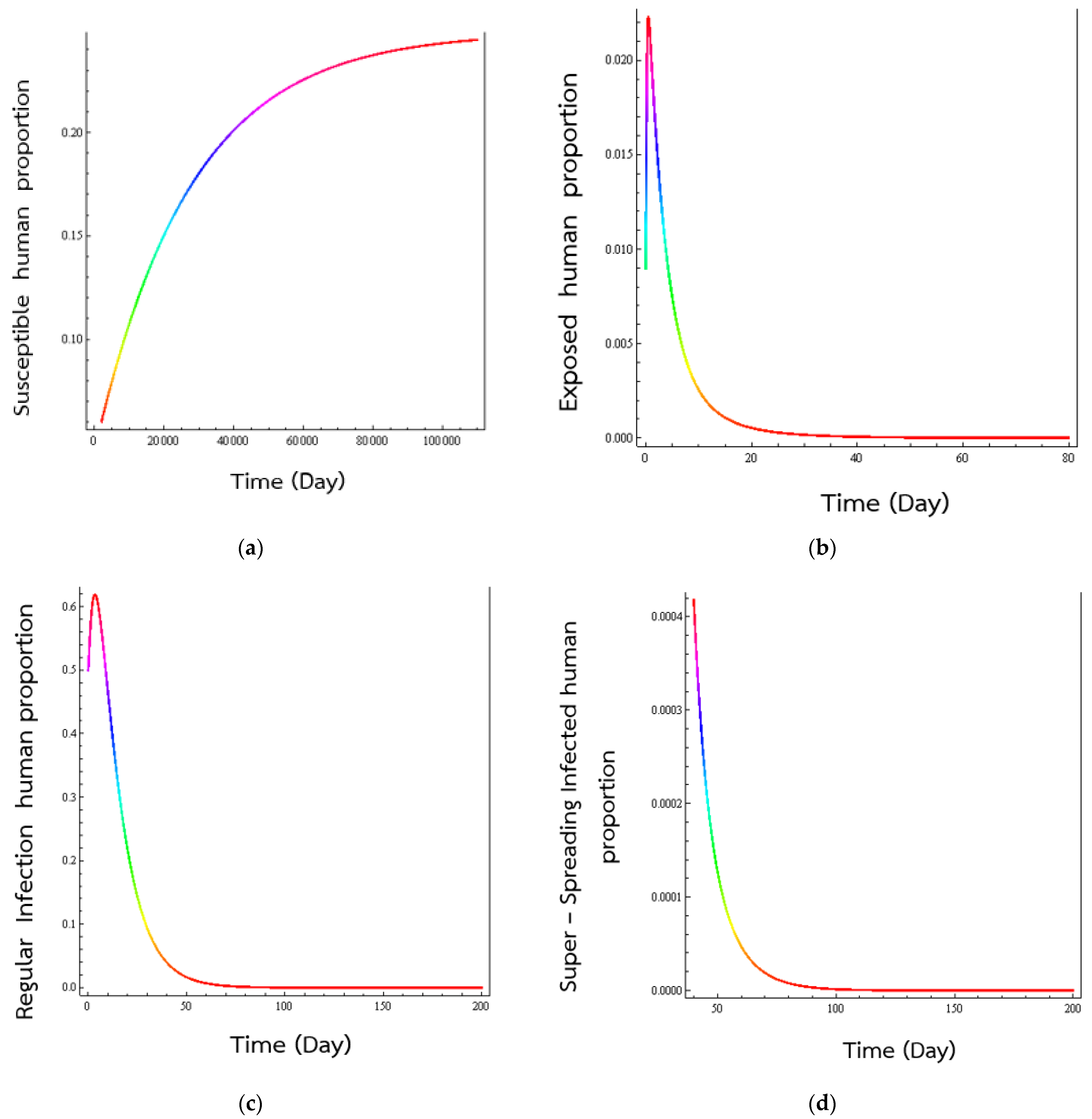
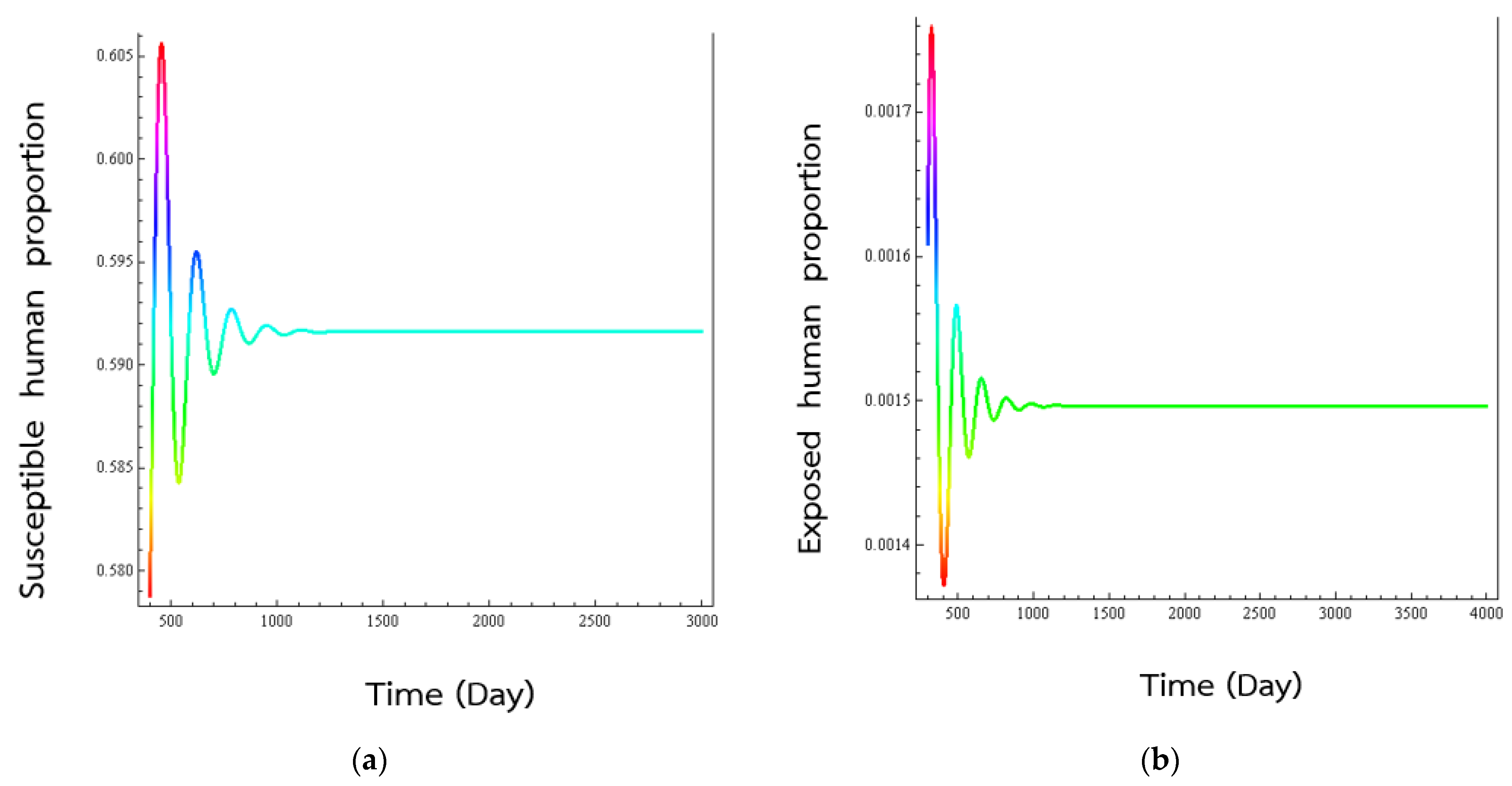
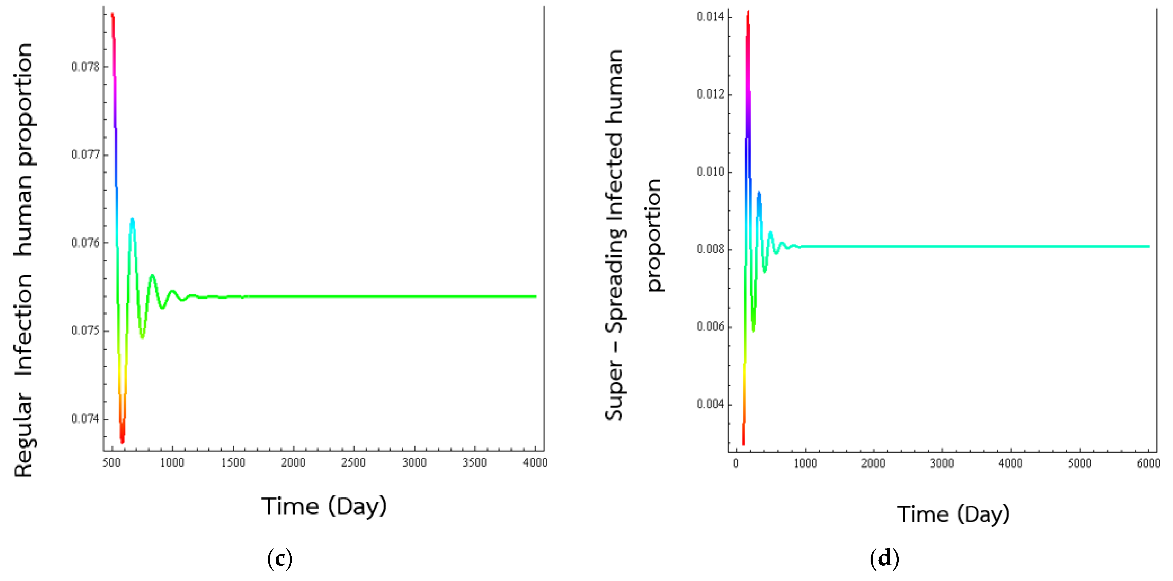
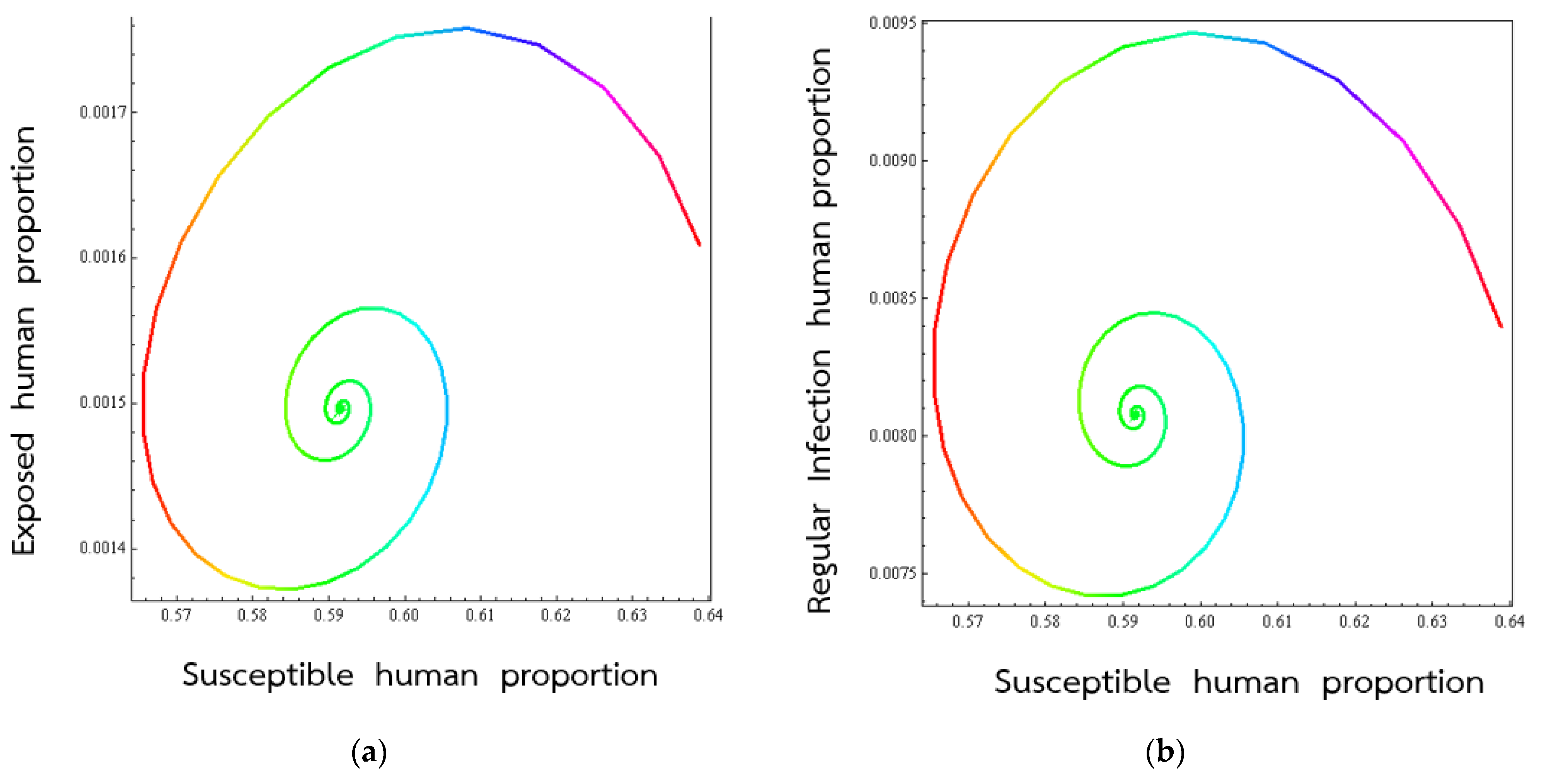
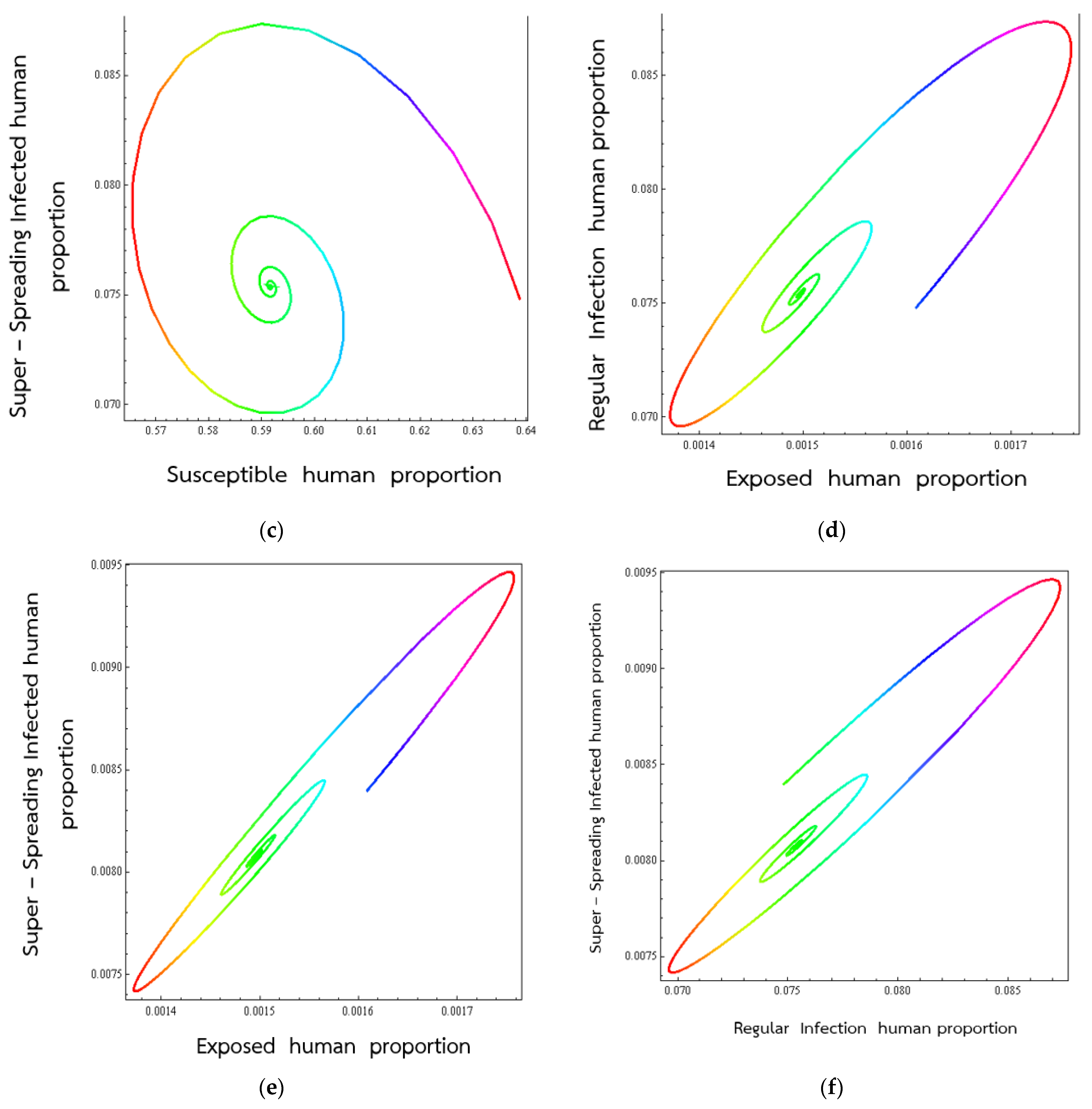
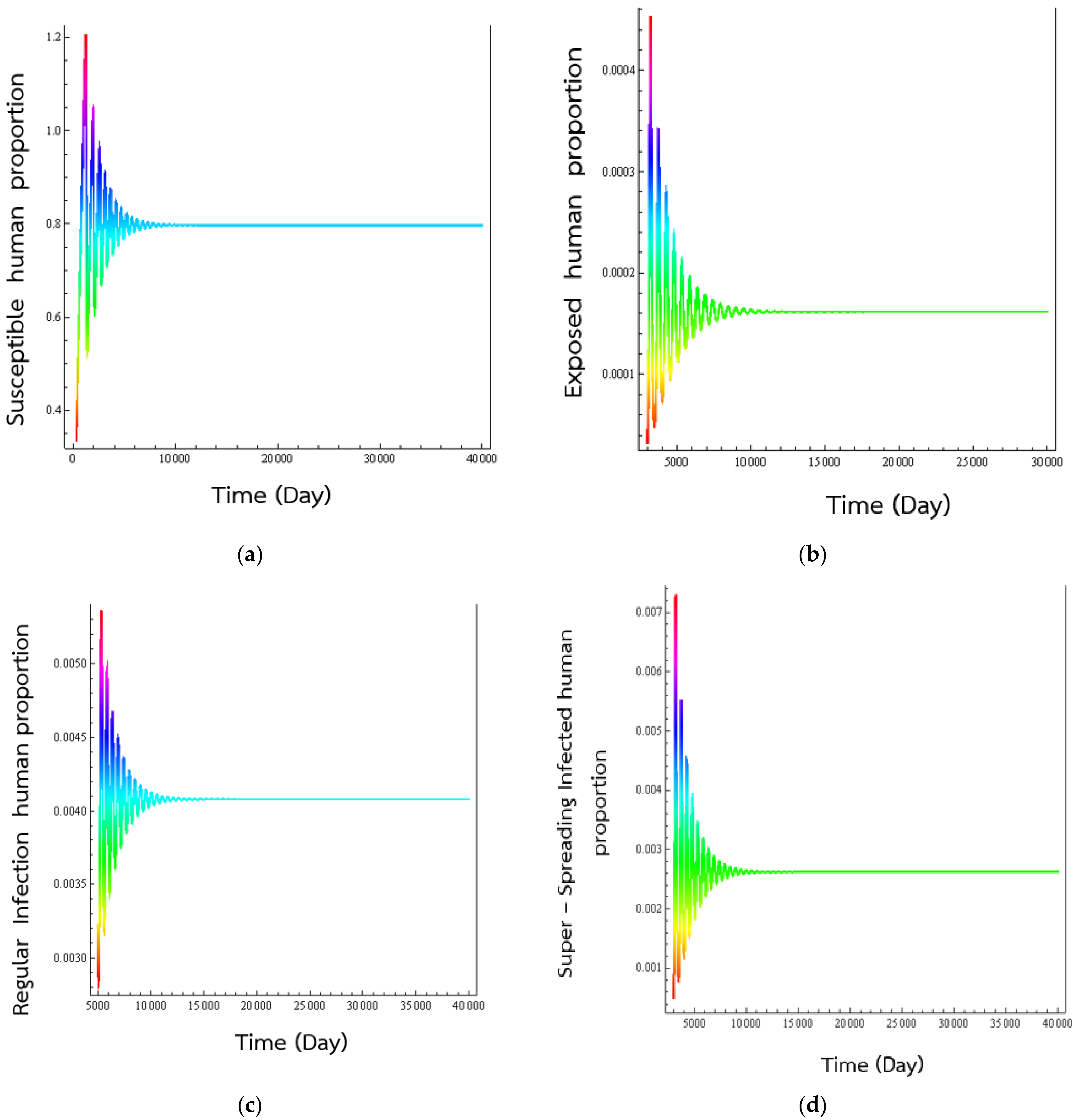
4. Numerical Results

The parameters used in the numerical simulation results are given in

Table 1. Parameters used in simulation for this model.

Parameters	Biological Meaning	Value
$b$	birth rate of human population	1/(365 × 75.65) per day [1]
$\mu$	death rate of human population	1/(365 × 75.65) per day [1]
$\beta$	transmission rate of virus between humans	0.1–0.9 per day [1] or [11] or [20,21]
$\eta$	incubation time of virus in humans	0.1–0.9 per day [1] or [11] or [20,21]
P	probability that a new case will be a regulated infected human	0.01–0.0009 [20,21,22]
$(1 - p)$	probability that a new case will be a super-spreading infected human	0.1–0.9999 [20,21,22]
r1	recovery rate of regular infected humans	0.01–0.9 [20,21,22]
$r_2$	recovery rate of super-spreading infected humans	0.1–0.7 [20,21,22]

. As we see, there are two numerical values listed (0.01 and 0.0009) except for the value of p, the percentage of exposed individuals who will develop a normal viral load. Using these values, these values would lead to $R_0 = 0.8302$ and 745.322. The first values of the basic reproduction would mean that the equilibrium state would be the disease-free state, while the second would be the endemic disease state. To see whether these predictions are true, we have numerically solved Equations (1) to (5) using the numbers listed in Table 1. Picking the set of lower values, we get the time behaviours in Figure 2, which shows the time evolutions of the various populations to their equilibrium values.

When the second set of numerical values, the basic production number becomes $R_0 = 745.332$, which is greater than one. According to Theorem 3, the disease endemic state ζ₂ will be globally asymptotically stable. Looking a Figure 3, we see that the plots of the evolutions of susceptible population, exposed population, normal infectious populations, and the super-spreader infected population show oscillatory behaviours as they approach their endemic values. Figure 4, show the trajectories of behaviours in two-dimensional space spiraling into the equilibrium epidemic state. The advantages of mathematical simulation studies of the behaviours of the endemic are that we can see the consequences of making changes in the practice of treating the illnesses without endangering the lives of people.

Figure 4 shows the course of the VSM endemic in various 2D space when the parameters in the mathematical description of the disease take on representative values. In the present case, we are looking at what happens when the percentage of exposed individuals become normal infected (develop into infected individuals having a normal (low) viral load).

The advantage of introducing the mathematical model of an endemic is that one can investigate through mathematical simulations the consequences of varying the treatment of the disease without there being any danger to the patients. One can see what happens if only some of the citizens are treated, or if some are given expensive treatments (such as drugs) and others are given inexpensive treatment (quarantine). One possible treatment would be to prevent exposed individuals (to RSV) from developing into super-spreaders. To see what the consequence are of lowering the values of p, we have first plotted the dependence of $R_0$ on the value of p. This dependence is shown in Figure 5. As we see, $R_0$ increases as p increases.

Examples of this can be seen in the cases where the diseases are the corona viruses, SARS, and MERS. In both of the endemics caused by these two viruses, the super-spreaders occurred when the evaluator was crowded [12] or the patient’s room was crowded and there was no ventilation to disperse the virus [13]. Normally, an exposed individual would be expected to develop into an individual carrying a normal viral load. Some individuals might carry a high viral load and if they meet one person, they would transmit the virus to the one person. However, if they get into a crowded situation and stay together for an extended period, they would become super-spreaders.

To show that changing the value of $R_0$ actually affects the dynamics of the epidemic, we have changed the value of p (to 0.04) and simulated the time evolutions of the various population classes. This change in the time evolutions of the different numerical solutions seen in Figure 5.

From Figure 6, we see that the solutions converge to the endemic disease state. Interestingly, the higher the percentage of exposed individuals becoming super-spreaders $(1 - p)$, the longer it takes for the oscillatory behaviour to stop.

5. Discussion and Conclusions

In this study, we have presented a mathematical model for the transmission of the respiratory syncytial virus (RSV) when there are super-spreader (infected individuals who can infect many people during one contact) present. We have included a super-infected class in the SEIR model, making it an SEI_rI_sR model [23,24,25,26,28,29,30]. We have analyzed this new model by performing a stability analysis of super-spreading transmission of the respiratory disease. The global stability of the transmission of respiratory disease was determined by using Lyapunov functions. We have obtained the basic reproductive number through the use of the spectral radius of the next generation matrix. The basic reproductive number is the threshold condition for investigating the stability of the solutions of model, which are shown in Figure 2. If $R_0 < 1$, then the disease-free equilibrium state is globally asymptotically stable, see Figure 3, Figure 4, and Figure 6. If $R_0 > 1$, then there is a unique endemic equilibrium state, which is globally asymptotically stable in the interior of the feasible region and the disease is present. This value is the approximation to the period of the solution [26,27,28,29,30,31,32]. L. Acedo et al. [9] consider the age structure of respiratory disease, with a focus on children under one year and children in general. With this model, the seasons will influence the transformation of this disease. Hogan et al. [29] consider a seasonal change of RSV by a seasonal forcing function and parameter space. Thus, their model is sensitive to the birth rate, transmission rate, and seasonality parameters, and can make a replica of RSV dynamics observed in different countries. From [8,29,31,32,33], and this model, the seasons will affect the change in the epidemic. In this case, the model also provided timely transmission of the inoculum and the body pod for the outbreak. We can see that the disease can be reduced when the parameters satisfied the conditions given in the above section.

References

1. World Health Organization. 2019. Available online: https://www.who.int/influenza/rsv/en/ (accessed on 18 April 2019).
2. Respiratory Syncytial Virus RSV. 2019. Available online: https://www.webmd.com/lung/rsv-in-babies (accessed on 6 May 2019).
3. Respiratory Syncytial Virus RSV. 2019. Available online: https://my.clevelandclinic.org/health/disease/8282respiratory-syncytial-virus-in-children-and-adults (accessed on 15 May 2019).
4. Respiratory Syncytial Virus RSV. 2019. Available online: https://medlineplus.gov/respiratorysyncytialvirusinfections.html (accessed on 15 May 2019).
5. Arenas, A.J.; Gonzalez, G.; Jodar, L. Existence of periodic solutions in a model of respiratory syncytial virus RSV. J. Math. Anal. Appl. 2008, 344, 969–980. [Google Scholar] [CrossRef] [Green Version]
6. Weber, A.; Weber, M.; Milligan, P. Modeling epidemics caused by Respiratory syncytial virus (RSV). Math. Biosci. 2001, 172, 95–113. [Google Scholar] [CrossRef]
7. Sungchasit, R.; Pongsumpun, P.; Tang, I.M. Environmental Impact on the Spread of Dengue Virus when two Mosquito Species Circulate. Far East J. Math. Sci. FJMS 2017, 101, 137–170. [Google Scholar] [CrossRef]
8. Acedo, L.; Diez Domingo, J.; Morano, J.A.; Villanueva, R.J. Mathematical modelling of respiratory syncytial virus (RSV): Vaccination strategies and budget applications. Epidemiol. Infect. 2001, 138, 853–860. [Google Scholar] [CrossRef] [PubMed]
9. Hall, C.B.; Geiman, J.M.; Douglas, R.G., Jr.; Meagher, M.P. Control of nosocomial respiratory syncytial viral Infections. Pediatrics 1978, 62, 728–732. [Google Scholar] [CrossRef]
10. Moore, H.C.; Jacoby, H.P.; Blyth, C.; Mercer, G. Modelling the seasonal epidemics of Respiratory Syncytial Virus in young children Submitted to Influenza and Other Respiratory Viruses among humans. Curr. Opin. Virol. 2013, 28, 142–151. [Google Scholar]
11. Gonzalez-Parra, G.; Rodríguez, D.M.; Villanueva-Micó, R.J. Impact of a New SARS-CoV-2 Variant on the Population: A Mathematical Modeling Approach. Math. Comput. Appl. 2021, 26, 25. [Google Scholar] [CrossRef]
12. Jeong, D.; Lee, C.H.; Choi, Y.; Kim, J. The daily computed weighted averaging basic reproduction number Rn0,k,ω for MERS-CoV in South Korea. Phys. A Stat. Mech. Its Appl. 2016, 451, 190–197. [Google Scholar] [CrossRef]
13. Pongsumpun, P.; Sungchasit, R.; Tang, I.M. Lyapunov Function for a Dengue Transmission Model where two Species of Mosquitoes are Present: Global Stability. Am. J. Appl. Sci. 2017, 14, 994–1004. [Google Scholar] [CrossRef] [Green Version]
14. Xu, X.; Yu, C.; Qu, J.; Zhang, L.; Jiang, S.; Huang, D.; Chen, B.; Zhang, Z.; Guan, W.; Ling, Z.; et al. Imaging and clinical features of patients with 2019 novel coronavirus SARS-CoV-2. Eur. J. Nucl. Med. Mol. Imaging 2020, 47, 1275–1280. [Google Scholar] [CrossRef] [Green Version]
15. Cha, M.J.; Chung, M.J.; Kim, K.; Lee, K.S.; Kim, T.J.; Kim, T.S. Clinical implication of radiographic scores in acute Middle East respiratory syndrome corona-virus pneumonia: Report from a single tertiary-referral center of South Korea. Eur. J. Radiol. 2018, 107, 196–202. [Google Scholar] [CrossRef] [PubMed] [Green Version]
16. Ohuma, E.O.; Okiro, E.; Ochola, R.; Sande, C.; Cane, P.A.; Medley, G.; Bottomley, C.; Nokes, D.J. The natural history of respiratory syncytial virus in a birth cohort: The influence of age and previous infection on reinfection and disease. Am. J. Epidemiol. 2012, 176, 794–802. [Google Scholar] [CrossRef] [PubMed]
17. Liu, X.; Stechlinski, P. Infectious Disease Modeling; Springer: Berlin/Heidelberg, Germany, 2017. [Google Scholar]
18. Kim, Y.; Cho, N. A Simulation Study on Spread of Disease and Control Measures in Closed Population Using ABM. Computation 2022, 10, 2. [Google Scholar] [CrossRef]
19. Van den Driessche, P.; Watmough, J. Reproduction numbers and sub-threshold endemic equilibria for compartmental models of disease transmission. Math. Biosci. 2002, 180, 29–48. [Google Scholar] [CrossRef]
20. Sungchasit, R.; Pongsumpun, P. Mathematical Model of Dengue Virus with Primary and Secondary Infection. Curr. Appl. Sci. Technol. 2019, 19, 154–178. [Google Scholar]
21. Athithan, S.; Ghosh, M.; Li, X.-Z. Mathematical modelling and optimal control of corruption dynamics. Asian Eur. J. Math. 2018, 11, 12. [Google Scholar] [CrossRef]
22. Liu, L.; Ren, X.; Liu, X. Dynamical Behaviours of an Influenza Epidemic Model with Virus Mutation. J. Biol. Syst. 2018, 26, 455–472. [Google Scholar] [CrossRef]
23. Esteva, L.; Vargas, C. Analysis of a dengue disease transmission model. Math. Biosci. 1998, 150, 131–151. [Google Scholar] [CrossRef]
24. Jin, Z.; Haque, M. Global Stability Analysis of an Eco—Epidemiological Model of the Salton Sea. J. Biol. Syst. 2006, 14, 373–385. [Google Scholar] [CrossRef]
25. Prathumwan, D.; Trach, K.; Chaiya, I. Mathematical Modeling for Prediction Dynamics of the Coronavirus Disease 2019 (COVID-19) Pandemic, Quarantine Control Measures. Symmetry 2020, 12, 1404. [Google Scholar] [CrossRef]
26. Diekmann, D.; Heesterbeek, J. Mathematical epidemiology of infectious disease: Model building, analysis and interpretation. In Wiley Series in Mathematical and Computational Biology; Wiley: Chichester, UK, 2000. [Google Scholar]
27. Lenhart, S.; Workman, J.T. Optimal Control Applied to Biological Models. In Mathematical and Computational Biology Series; Chapman & Hall/CRC: Boca Raton, FL, USA, 2007. [Google Scholar]
28. Hogan, A.B.; Glass, K.; Moore, H.C.; Anderssen, R.S. Exploring the dynamics of respiratory syncytial virus 2 (RSV) transmission in children. Theor. Popul. Biol. 2016, 110, 78–85. [Google Scholar] [CrossRef] [PubMed]
29. Moore, H.C.; Jacoby, P.; Hogan, A.B.; Blyth, C.C.; Mercer, G.N. Modelling the Seasonal Epidemics of Respiratory Syncytial Virus in Young Children. PLoS ONE 2014, 9, e100422. [Google Scholar] [CrossRef] [PubMed] [Green Version]
30. Keeling, J.M.; Rohani, P. Modeling Infectious Diseases in Humans and Animals; Princeton University Press: Princeton, NJ, USA, 2008. [Google Scholar]
31. Paynter, S.; Yakob, L.; Simões, E.A.F.; Lucero, M.G.; Tallo, V.; Nohynek, H.; Ware, R.S.; Weinstein, P.; Williams, G.; Sly, P.D. Using Mathematical Transmission Modelling to Investigate Drivers of Respiratory Syncytial Virus Seasonality in Children in the Philippines. PLoS ONE 2014, 9, e90094. [Google Scholar] [CrossRef]
32. Hogan, A.B.; Glass, K.; Moore, H.C.; Anderssen, R.S. Age Structures in Mathematical Models for Infectious Diseases, with a Case Study of Respiratory Syncytial Virus. In Applications + Practical Conceptualization + Mathematics = fruitful Innovation; Springer: Tokyo, Japan, 2015; pp. 105–116. [Google Scholar] [CrossRef]
33. Hattaf, K.; Yousfi, N. Modeling the Adaptive Immunity and Both Modes of Transmission in HIV Infection. Computation 2018, 6, 37. [Google Scholar] [CrossRef] [Green Version]
Figure 1. Diagram for the dynamical transmission of respiratory disease. In the above flow chart, the variables are: S is the number of susceptible human population; E is the number of exposed human population; I r is the number of normal infected human; I s is the number of super-spreading infected human; I is the total infected human population, I = I r + I s ; R is the number of recovered human population.
Computation 10 00120 g001
Figure 2. Numerical solution of systems (1)–(5), time series of (a) susceptible human population, (b) exposed human population, (c) normal infected humans, and (d) super-spreading infected humans. The numerical values of the parameters are listed in Table 1 and these are just possible values and have no significance. The simulated human populations converge to the disease-free state ζ 1 *   (   0.2485 , 0 , 0 , 0 ) when R 0   =     0.8302       <     1 .
Computation 10 00120 g002
Figure 3. Numerical solution of systems (1)–(5), time series of (a) susceptible human population, (b) exposed human population, (c) regular infected humans, and (d) super-spreading infected humans to the transmission of respiratory disease. The numerical values of the parameters are values in the second column in Table 1. The values are representative values and have no medical significance and were picked in order for R 0 = 745.322 > 1 . The percentage of exposed individual would became normal infected individual was set at p = 0.7. As is seen, the simulations have the solutions converging to the disease endemic state, which is true according to Theorem 3. The simulated human populations converge to the endemic equilibrium states ζ 2 * = ( S * , E * , I r * , I s * ) at (0.59161, 0.00145, 0.07539, 0.00807).
Computation 10 00120 g003aComputation 10 00120 g003b
Figure 4. Trajectories of respiratory disease for the solutions equation approach to the endemic state onto (S, E) (a), (S, Ir) (b), (S, IS) (c), (E, Ir) (d), (E,Is) (e), (Ir, IS) (f), respectively.
Computation 10 00120 g004aComputation 10 00120 g004b
Figure 5. Dependence of R 0 on p (probability that a new case will be a normal infected human) value changes, the R 0 tends to increase.
Computation 10 00120 g005
Figure 6. Numerical solution of Equations (1)–(5) where p = 0.04. Time series behave of (a) susceptible human population, (b) exposed human population, (c) regular infected humans, and (d) super-spreading infected humans to the transmission of respiratory disease. The simulated human populations converge to the endemic equilibrium states ζ 2 * = ( S * , E * , I r * , I s * ) at (0.79734, 0.00016, 0.00408, 0.00262).
Computation 10 00120 g006