Article

An Anomaly Detection Model for Oil and Gas Pipelines Using Machine Learning

by
Sumayh S. Aljameel
1,
Dorieh M. Alomari
2,*,
Shatha Alismail
2,
Fatimah Khawaher
2,
Aljawharah A. Alkhudhair
2,
Fatimah Aljubran
2 and
Razan M. Alzannan
2
1
Department of Computer Science, College of Computer Science and Information Technology, Imam Abdulrahman Bin Faisal University, P.O. Box 1982, Dammam 31441, Saudi Arabia
2
Department of Computer Engineering, College of Computer Science and Information Technology, Imam Abdulrahman Bin Faisal University, P.O. Box 1982, Dammam 31441, Saudi Arabia
*
Author to whom correspondence should be addressed.
Computation 2022, 10(8), 138; https://doi.org/10.3390/computation10080138
Submission received: 2 July 2022 / Revised: 27 July 2022 / Accepted: 9 August 2022 / Published: 10 August 2022

Abstract

:
Detection of minor leaks in oil or gas pipelines is a critical and persistent problem in the oil and gas industry. Many organisations have long relied on fixed hardware or manual assessments to monitor leaks. With rapid industrialisation and technological advancements, innovative engineering technologies that are cost-effective, faster, and easier to implement are essential. Herein, machine learning-based anomaly detection models are proposed to solve the problem of oil and gas pipeline leakage. Five machine learning algorithms, namely, random forest, support vector machine, k-nearest neighbour, gradient boosting, and decision tree, were used to develop detection models for pipeline leaks. The support vector machine algorithm, with an accuracy of 97.4%, overperformed the other algorithms in detecting pipeline leakage and thus proved its efficiency as an accurate model for detecting leakage in oil and gas pipelines.

1. Introduction

In the oil and gas industry, various problems and anomalies could damage oil and gas pipelines, which could ultimately result in human injuries and financial loss. A few examples of these anomalies include corrosion, leakage, and rust. Oil and gas leakage can be dangerous for people’s health and the surrounding environment. Additionally, leakage of gases such as isobutane and propane into the atmosphere is very harmful because of their effect on ozone depletion or global warming. Therefore, a number of studies have been published to develop a gas leak detection model [1]. Recent advancements in artificial intelligence (AI) and data sensing have created new opportunities to solve challenging problems in environmental monitoring, such as solid waste, air, and wastewater pollution [2].
AI is one of the most useful technologies in this age. It encompasses a wide array of technologies, including machine learning (ML) and deep learning (DL), which can be used in various applications such as industry, health, economies, etc. [3]. Furthermore, AI plays a pivotal role in improving the oil and gas industry, and various ML- and DL-based AI techniques have been used to detect anomalies in pipelines. In previous studies, several deep learning models were implemented to detect oil and gas leakage in pipelines. In ref. [4], the authors aimed to reduce environmental pollution by developing an ML model to detect oil and gas leakage. The model resulted in an accuracy of 98.57%. At the same time, the model presented in ref. [5] resulted in an accuracy of 99.4% in detecting leakage. In another study, a mask region-based convolutional neural network (Mask R-CNN) and the Visual Geometry Group 16 (VGG-16) model were employed to locate and identify oil spills in pipelines [6]. The model resulted in an accuracy of 93%, which is higher than the model of ref. [7], which also used CNN to demonstrate recent findings in infrared (IR)- and acoustic-based techniques for leak detection. Additionally, the method presented alternative methods such as temperature profiling, ground-penetrating radar, and photoacoustic sensing techniques.
Weather conditions and extreme temperatures increase the potential for pipeline damage. Oil and gas pipelines are usually located in remote and harsh areas, and thus, it is difficult to rely on humans to monitor oil and gas pipelines physically and ascertain leakage positions. The adoption of AI and the internet of things (IoT) can produce pipeline leak detection systems and safety applications that benefit the oil and gas industry. In a study, IoT cameras from various locations on the pipelines were used to generate video clips, which were ultimately analysed by implementing the CNN to detect oil and gas leakage [8].
In this paper, the authors propose an ML model to detect oil and gas leakage in pipelines. This work provides a comparative analysis of five ML models to detect pipeline leakage using an industrial dataset. Additionally, several optimisation techniques are applied to this model to attain the highest accuracy. The model detects leakage using three operational parameters, namely, temperature, pressure, and flow rate. The applied models are compared in terms of precision, recall, F1-score, accuracy, and receiver operating characteristic-area under the curve (ROC-AUC).
The significant contributions of this study are:
  • An automated system is developed to identify anomalies in the oil and gas pipeline;
  • A comparison of five ML algorithms to detect pipeline leakage using industrial datasets is performed;
  • Evaluation methodology in terms of accuracy, precision, recall, F1-score, accuracy, and ROC-AUC is proposed;
  • An optimisation technique is used to increase the performance of the proposed models.
Enhancing the economy of several large companies in the oil and gas industry will enhance the economy in many counties, such as Saudi Arabia. As stated earlier, the authors developed an ML-based novel solution for pipeline leak detection. Five ML models, namely, support vector machine (SVM), k-nearest neighbours (KNN), random forest (RF), gradient boosting (GB), and the decision tree (DT) algorithm, were used and compared. The proposed model is anticipated to add many benefits to the Saudi market and even to the global market.
The remainder of this paper is organised as follows. Section 2 summarises the related studies in leakage detection systems using AI techniques. Section 3 introduces the proposed methodology. Section 4 discusses the results of the proposed model. Finally, Section 5 presents the concluding remarks and some suggestions for future work.

2. Related Work

Wang et al. [4] proposed a model that uses temperature information fusion and distributed vibration to detect oil and gas pipeline leaks depending on the measurement ability of distributed optical fibre sensors. Their prime goal was to reduce environmental pollution and economic loss by monitoring and timely recognising pipeline leakage. The researchers used five different classification models, namely naive Bayes, KNN, DT, RF, and backpropagation neural networks. The models can recognise the normal operation, interference, and state of leakage. A comparison was made between the performance of the classifiers, and RF exhibited the most superior performance with five vibration attribute values and six temperature attribute values. The RF classifier reached 98.57% in recognising the oil and gas pipeline leakage.
Lu et al. [9] proposed a model that can extract the features of pipelines to detect leakage. The continuous expansion of pipeline networks and the lack of research in the field of pipeline leakage recognition using leak features were the two main driving factors in this study. A combination of variational mode decomposition and SVM was proposed to extract pipeline leakage characteristics. The researchers employed three kernel functions, namely the polynomial kernel, linear kernel, and radial basis function (RBF) kernel. The researchers found RBF to be the optimum kernel function with 96% accuracy, 92% specificity, and 100% sensitivity. In addition to the effectiveness of the proposed method in the experimental data, the researchers assessed the method in practical application.
Xiao [5] proposed a model that uses acoustic signals to detect gas pipeline leakage. The main goal of this research was to protect society from damage caused by gas pipeline leaks. The proposed method to detect gas pipeline leaks employed SVM and wavelet transform. The latter was used to preprocess acoustic sensor signals, and the entropy-based algorithm was used to select the optimal wavelet basis, followed by the extraction of leak-related information from the acoustic signals. The Relief-F algorithm was used for feature selection, and its output was fed as an input to the SVM model to detect gas pipeline leakage. The proposed method proved its effectiveness as it reached 99.4% in classifying the events leading leaks or no leaks using the three most discriminative features and 95.6% using the five most discriminative features.
De Kerf et al. [7] proposed a model for detecting oil leakage inside a port environment using thermal IR cameras and unmanned aerial vehicles (UAV). The IR images were necessary to detect oil leakage during night-time. The researchers presented a method to annotate the red, green, and blue (RGB) images and match them with the IR images to collect the dataset. The collected images were resized and used to train a CNN. Once the network was trained, it enabled the frequent inspection of oil leakage on the water at a low cost. During the test stage, the researchers were able to detect oil leakage on water successfully with an accuracy of 89%. The implemented solution can decrease the cleaning cost of oil leakage in water, minimise human interaction during the process, and increase the detection rate. Further improvements could be applied in the future using other camera technologies and more advanced preprocessing techniques.
Ghorbani and Behzadan [6] developed different models for oil spill detection to help people take adequate actions effectively and immediately and mitigate the overall damage. Two deep learning models, mask R-CNN and VGG-16, were used to locate and identify oil leakage. A dataset was created through web mining, and it contained 1292 images. The VGG-16 model was used for the image classification process to predict oil leakage via an image, and it reached an accuracy of 93%. The mask R-CNN model was use for segmentation to detect oil leakage and to mark the boundaries of the spill at the pixel level and yielded average recall and precision of 70% and 61%, respectively. The resultant models can create more opportunities for advancing the current practices of combining data analytics and AI into up- and downstream operations in the oil and gas industry, as well as detecting environmental pollutants using non-intrusive techniques. To increase the likelihood of technology adoption by the oil and gas industry and reduce the implementation cost, the researchers worked with RGB images as inputs as the used drones contain RGB cameras. With certain modifications, the same method can be used for other types of inputs (e.g., thermal and infrared images).
Melo et al. [10] introduced different techniques for the detection of natural gas leakage in oil facilities. Different CNNs were proposed to detect the leakage of natural gas. The dataset that they used contained 2980 images and was divided into two classes, namely, ‘with leak’ (980 images) and ‘without leak’ (2000 images). The performance of 27 different CNN models was evaluated to achieve the best accuracy. The model with the best performance had the following characteristics: SGDM optimisation algorithm, 18 convolution layer architecture, and dropout regularisation technique, and it yielded an accuracy of 99.78% and a false-negative rate of 0%. In the future, the researchers plan to evaluate the generalisation ability of the model on unseen images of different types.

3. Methodology

The methodology that was followed during this study includes important steps for building an ML model. The first step involves the collection of the required dataset and a preprocessing phase. The second step involves training the proposed model and evaluating its performance. A more detailed description of the methodology is included in this section. Figure 1 summarise the methodology of this study.

3.1. Data Collection

An open-source dataset obtained from GitHub was used in this study [11]. The dataset was proposed for public use for studies such as ML and other statistical studies. It was originally proposed with a regression target class of the corrosion defect. The dataset contains eight features and 10,293 instances, and it contains numerical attributes. Additionally, the dataset could be used for regression and classification problems, and it is split into training and testing sets. Table 1 describe its various features.

3.2. Data Preprocessing

The success of ML algorithms depends on various factors. The first factor is the quality and representation of the instances on the dataset. The work in the training phase needs to have reliable data that does not contain noisy or redundant values. Data preparation and filtering are important steps in processing ML problems. Data preprocessing includes data cleaning, features normalisation, and extraction [12].

3.2.1. Label Binarizing

There is a noteworthy difference between regression and classification problems. The former is concerned with predicting a quantity, while the latter is concerned with predicting a label. Thus, label binarizing was used in this study to convert a regression problem into a classification problem [13].
The authors converted the target attribute from regression to classification to build the said models. The values less than or equal to 0.211 were treated as ‘low’, and the values greater than 0.211 were treated as ‘high’. Figure 2 illustrate label binarizing. The figure shows the number of instances in each class; the ‘high’ class contains 5491 samples, whereas the ‘low’ class contains 4801 samples.

3.2.2. Features Scaling

Feature scaling is a technique used to normalise the range of independent features or variables of data. Feature scaling is performed during the preprocessing stage, and it is also known as data normalisation. Feature scaling can be carried out using either data standardisation or normalisation [14].
Data normalisation improves the performance of the ML model, as well as generates an accurate prediction model that predicts with high accuracy. It is also known as min–max normalisation or min–max scaling. It rescales the range of features within the range [0,1]. Normalisation uses a general formula given as:
x = x m i n x m a x x m i n x .
Here, x’ is the new value, x is the original values, min(x) and max(x) are the minimum and the maximum values of the feature, respectively [14,15].

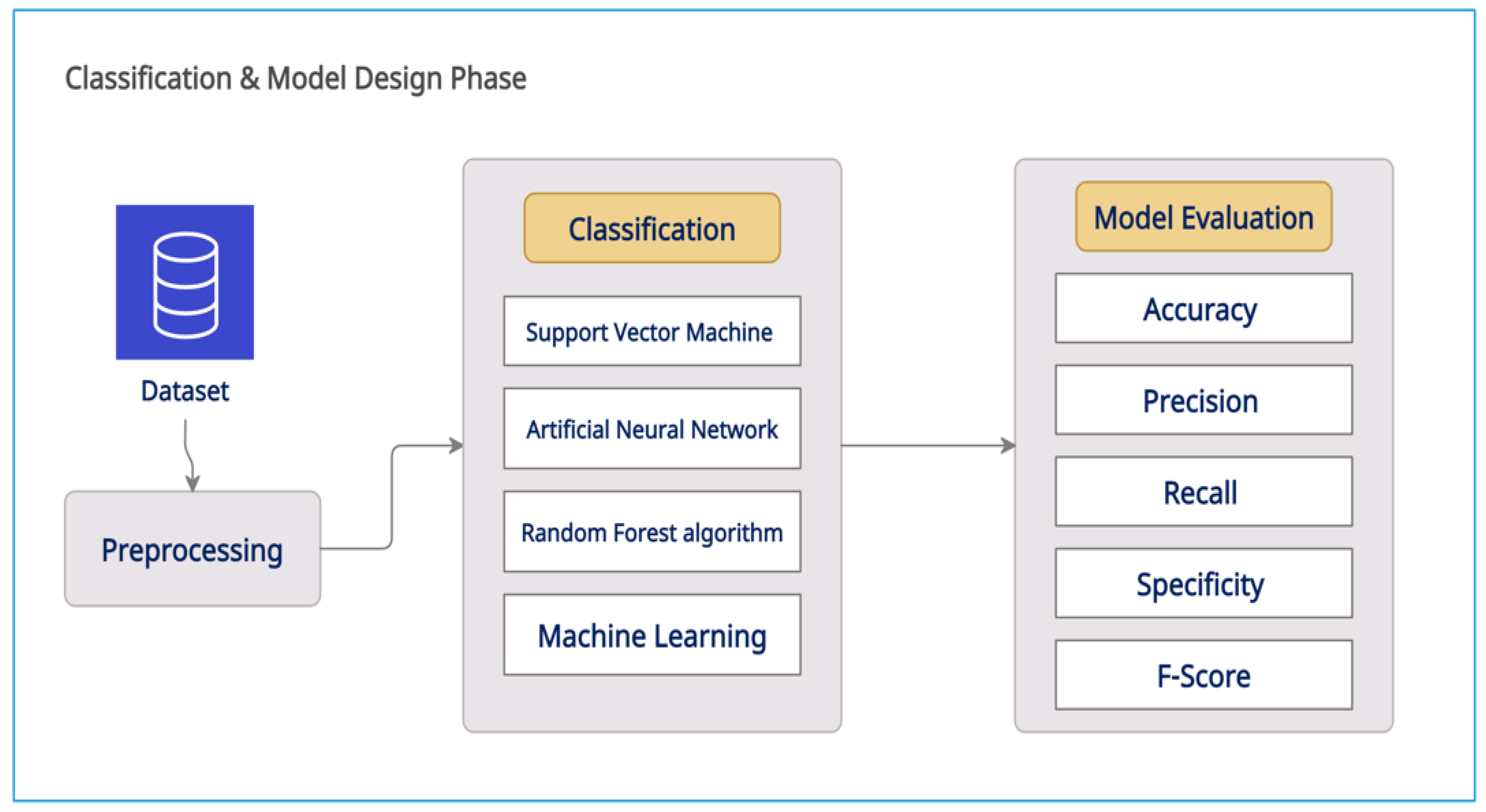
3.3. Classification and Model Design

After preprocessing and cleaning the dataset, the authors built ML models. To build the models, the dataset was divided into samples to train and test the model. The performance of the model was measured in terms of the accuracy of the model on the testing sample [16]. The most common approaches for splitting the dataset are 7:3 (training:testing) and 10-fold cross-validation (CV). In the 7:3 approach, the dataset is divided into two samples, one for training and the other for testing. The training sample represents 70% of the dataset, and the testing sample is the remaining 30% [17]. The training sample is used to train the model and enhance its ability to learn the complexity behind the features of the dataset, while the testing sample is used to measure the performance of the model on unseen data. In a 10-fold CV, the dataset is divided into 10 folds, and the model is trained 10 times. In each iteration, nine folds are used to train the model, and the remaining fold is used to test its performance. The average accuracy is calculated at the end of this process [18].

3.3.1. Support Vector Machine

SVM, a supervised learning approach, is one of the most popular and simplest ML techniques because its solutions are often perfect and unique. In addition, it has good generalisability due to the principle of structural risk minimisation. This principle reduces the confidence interval while keeping the values of training error constant [19,20]. SVM can be used in both regression and classification prediction because it maximises the predictive accuracy rate through the use of ML theory and avoids data over-fitting [21]. When using SVM, it must be considered that it is a nonparametric technique (scattered technique), as its use requires storing all the training data in memory during the training phase to determine the model’s parameters. As for future forecasting, support vectors are relied upon, which are a subset of training cases [19]. As shown in Figure 3, support vectors are represented by points scattered around a straight line called the hyperplane, a single line used to separate and classify data. The idea of SVM is to find a hyperplane that achieves maximum separation [20]. Furthermore, the representation of this hyperplane varies depending on whether the data can be easily separated, which results in two types of SVM classifiers, linear and nonlinear. Several hyperplanes are shown in Figure 3, and an SVM will select the best among them.

3.3.2. Decision Tree

DT is a supervised algorithm used to solve both classification and regression problems. It is used to create a predictive model that predicts the value or category of the target, and this is carried out by teaching the model the simple decision rules derived from the training data. In this algorithm, the process of predicting the class name of any record starts from the root of the tree. The prediction is developed by comparing the value of the tree root attribute with the attribute of the record whose class name is to be predicted. Based on the comparison, the moves between the following nodes depend on the branch corresponding to that value [22]. Figure 4 show the DT classifier.

3.3.3. Random Forest

RF is one of the most widely used supervised ML algorithms. It is responsible for building an ensemble of decision trees and then training them using the bagging method; therefore, it is called a ‘random forest’ [24]. Bagging is a concept that aims to integrate several learning models to improve the overall performance of the achieved result [24]. In recent years, this algorithm has garnered popularity owing to its simplicity and versatility in being applied to both classification and regression models. Moreover, the isolated tree structure in the forest can predict the class, which is basically the class that obtains the highest number of votes within the model [24]. Figure 5 depict the functioning of the RF algorithm.
It is proven that multiple unlinked trees working together is more efficient than a single isolated tree [26]. Because of this, the trees tend to protect and shield each other from defects that may develop within the forest structure. This protection is maintained while they do not walk within the same path. An interesting mystery involves the method by which the RF algorithm ensures that the behaviour of these individually isolated trees does not overly correlate with other tree structures within the model.
Finally, random forest is a very useful and versatile algorithm that can be used for both regression and classification. Furthermore, if there are enough trees in the forest, the overfitting problem is solved, and highly accurate prediction results are achieved [27]. An unfavourable aspect of the RF algorithm is the fact that, when a lot of trees are used, the algorithm can become inefficient and extremely slow for real-time predictions. The use of more trees is required for a much more accurate prediction, resulting in a slower model [28]. In most real-world applications, RF works well, but there can be cases when run-time performance is critical, and other approaches may be more effective [28].

3.3.4. K-Nearest Neighbour

KNN is one of the supervised algorithms used to solve both classification and regression problems. This algorithm is known as the lazy learning algorithm because it only stores data during the training phase without performing any arithmetic operations on it. This algorithm creates a predictive model that predicts the correct category of test data by finding the distance between it and the training data. The algorithm determines the k number of points closest to the test data. Next, it calculates the probability of the test data falling into the category k group, and finally, it chooses the category that achieves the highest probability. The parameter k represents the number of neighbours’ relatives included in the voting process. The distance between point data and its nearest neighbour can be calculated as Euclidean distance, Manhattan distance, Hamming distance, Minkowski distance, etc. Among these distance metrics, Euclidean distance is the most widely used [29]. Figure 6 show the Euclidean distance of the KNN classifier.
Figure 6 depict a graph containing two classes of datasets A and B, and a new data point for which the class it might belong to needs to be predicted. Using the Euclidean distance equation with a value of k equal to 5, the distance between the data points can be calculated to obtain the nearest neighbours [30]. Figure 7 show the classification of KNN.
As shown in Figure 7, the three nearest neighbours are from class A, and the two nearest neighbours are from class B, so the new point belongs to class A [30].

3.3.5. Gradient Boosting

GB is a supervised algorithm used to build a predictive ML model. In the process of integrating individual decision trees into the algorithm, a method called ‘reinforcement’ is used. Reinforcement means developing a strong learner by merging several learning algorithms of weak learners into a single chain. The DT in this algorithm represents weak learners. The model of this algorithm is characterised by high efficiency and accuracy because each tree inside it works to fix the errors of the tree that precedes it. However, the sequential increase of trees inside the algorithm improves its performance but slows the learning process. In addition, the model relies on the loss function for residual detection. For example, the logarithmic loss is used in classification and regression tasks. Figure 8 show how the GB algorithm works [31].

3.4. Parameter Tuning

Hyperparameters are the optimal values that define the model architecture. Hyperparameter tuning refers to the process of searching and selecting the optimal parameter and creating the model architecture. The value of the hyperparameter cannot be estimated from data and must be set before initiating the learning process [32].

Grid Search

Grid search is a basic hyperparameter tuning method. GridsearchCV enables the grid search, where it generates candidates from a grid of parameter values. Furthermore, the GridsearchCV instance implements the usual estimator application programming interface. As a result of fitting the grid search on the dataset, the best combination is retained after all the possible combinations of parameter values are evaluated [33]. Table 2 show the optimal values for each parameter.

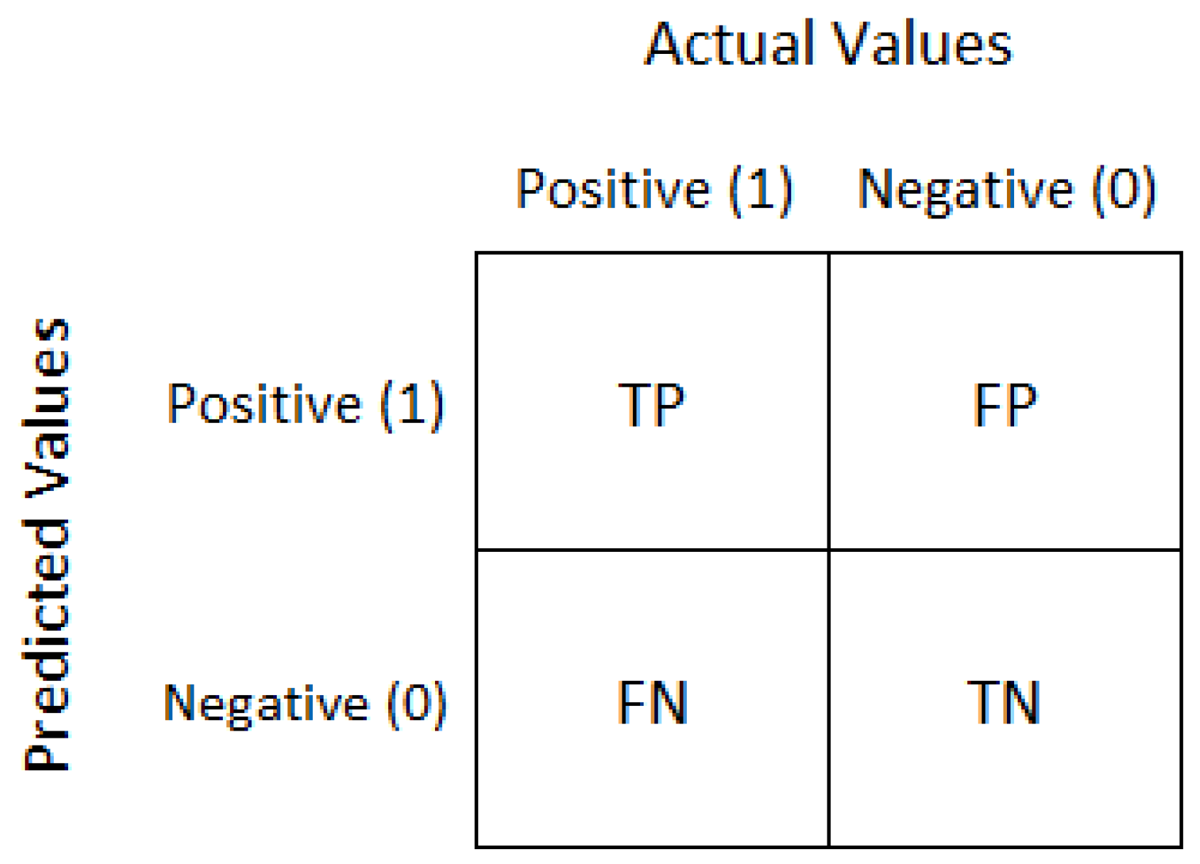
3.5. Evaluation Metrics

In addition to accuracy, other metrics, namely, the confusion matrix, precision, recall (or sensitivity), specificity, F-score, and receiver operator characteristic–area under the curve (ROC-AUC), are used to measure the performance [34].
The confusion matrix measures the performance of the ML model by comparing the predicted values with the real values. Figure 9 show a confusion matrix for binary problem classification [35].
The symbols TP, TN, FP, and FN indicate true positive, true negative, false positive, and false negative, respectively [35].
A c c u r a c y = T P + T N T P + T N + F P + F N .  
Accuracy represents the percentage of the truly predicted samples among all the samples in the testing set [37].
P r e c i s i o n = T P T P + F P .
Precision represents the percentage of the truly predicted samples of the positive class among all the positive predictions [37].
R e c a l l = T P T P + F N .  
Recall (also known as sensitivity) represents the percentage of the positive samples that were correctly predicted among all the real positive samples [37].
S p e c i f i c i t y = T N T N + F P .  
Specificity represents the percentage of the negative samples that were correctly predicted among all the real negative samples [37].
F 1 S c o r e = 2 × P r e c i s i o n × R e c a l l P r e c i s i o n + R e c a l l .
The F1-score represents the average of the truly predicted samples of the positive class (precision) and the positive samples that are correctly predicted (recall). It is used to evaluate the balance of the model’s predictions among the two classes [34,37]. ROC-AUC plots the probability of TP and FP at various thresholds. Thus, it shows the ability of the model to distinguish between the two classes [38].

4. Results and Discussion

Table 3 show the results of evaluating the models on the oil and gas pipeline leakage dataset prior to parameter optimisation.
As evident from Table 3, the SVM model resulted in the best performance with an accuracy of 96.1%, followed by the RF model with an accuracy of 91.56%. The other models resulted in accuracy below 90%. Figure 10 show the confusion matrix for the SVM model.
The confusion matrix shows that the model misclassified 178 samples in the ‘high corrosion’ class (0) and 224 samples in the ‘low corrosion’ class (1). This means the model’s ability to identify high corrosion is very high, and this is needed to predict pipeline leakage.
Table 4 show the results of evaluating the models on the oil and gas pipeline leakage dataset after the parameter optimisation.
As shown in Table 4, the performance of all the models is improved after parameter optimisation. The SVM model resulted in the best performance with an accuracy of 97.43%, followed by the RF model with an accuracy of 91.81%. The accuracy of RF did not improve very well compared with the previous experiments. The performance of the GB model was significantly improved from 87.39% to 90.25%. Figure 11 show the confusion matrix for the SVM model.
The confusion matrix shows that the model misclassified 119 samples in the ‘high corrosion’ class (0) and 145 samples in the ‘low corrosion’ class (1). The number of misclassified samples was reduced in both classes. Although the accuracy of the SVM model was improved by 1% after optimisation, the confusion matrix shows a great improvement in the model’s ability to distinguish between the two classes. Moreover, the model’s ability to identify high corrosion is very high, and this is needed to predict pipeline leakage. Figure 12 show the ROC-AUC curve of the SVM model.
The ROC-AUC curve shows that the ability of the model to differentiate between low and high corrosion is very high (0.97), which means that the model can be used in real-world applications with a high level of confidentiality.

5. Conclusions

In this paper, one of the most prominent issues faced by most oil and gas companies is highlighted, which is the problem of oil and gas leakage inside pipelines. Several previous studies were reviewed to benefit from some proposed solutions to solve the leakage problem and identify which algorithms can be used. The appropriate dataset was found, several predictive models were built using several ML algorithms, and then a comparison was made between them, choosing the best one in terms of performance. During the stage of evaluating models on the dataset of oil and gas pipeline leakage, two experiments were conducted, the first before parameter optimisation and the second after that. The results of the first experiment showed that all the proposed models resulted in good performance in anomaly detection, with performance of more than 83% in all the evaluating matrices. In comparison, the SVM model outperformed the rest of the models in performance with an accuracy of 96.1%, followed by the RF model with an accuracy of 91.56%. In the second experiment of the optimized models, there was a significant improvement in the performance of all the models. The SVM model is still considered the best among the rest of the models, with an accuracy of 97.43% and 97% in precision, recall, f1-score, and ROC-AUC. SVM was followed by the RF model with an accuracy of 91.81% and 92% in all other matrices. The confusion matrix shows the model’s ability to detect corrosion and distinguish between the two classes of high and low corrosion. According to these results, the proposed model achieved good performance in the industrial data that was used, achieving the goal of this study to be used in the real world.
Using the proposed models, it is possible to develop systems capable of effectively identifying the unusual event of oil and gas pipeline leakage, thus facilitating the proper operation of the industry and avoiding any potential damage to the industrial companies and the surrounding environment. The only difficulty in this study was collecting a real dataset from oil and gas companies for building the proposed model. For future work, a real dataset from oil and gas companies will be used to build the models. In addition, DL techniques will be used.

Author Contributions

Conceptualisation, S.S.A.; methodology, S.S.A., D.M.A., S.A., F.K., A.A.A., F.A. and R.M.A.; software, D.M.A., S.A., F.K., A.A.A., F.A. and R.M.A.; validation, S.S.A., D.M.A., S.A., F.K., A.A.A., F.A. and R.M.A.; formal analysis, S.S.A., D.M.A., S.A., F.K., A.A.A., F.A. and R.M.A.; investigation, S.S.A., D.M.A., S.A., F.K., A.A.A., F.A. and R.M.A.; resources, D.M.A., S.A., F.K., A.A.A., F.A. and R.M.A.; data curation, D.M.A., S.A., F.K., A.A.A., F.A. and R.M.A.; writing—original draft preparation, D.M.A., S.A., F.K., A.A.A., F.A. and R.M.A.; writing—review and editing, S.S.A., D.M.A., S.A., F.K., A.A.A., F.A. and R.M.A.; supervision, S.S.A.; project administration, S.S.A.; funding acquisition, S.S.A., D.M.A., S.A., F.K., A.A.A., F.A. and R.M.A. All authors have read and agreed to the published version of the manuscript.

Funding

This research received no external funding.

Institutional Review Board Statement

Not applicable.

Informed Consent Statement

Not applicable.

Data Availability Statement

Publicly available datasets were analyzed in this study. This data can be found here: [https://github.com/Abimbola-ai/Oil-and-gas-pipeline-leakage].

Conflicts of Interest

The authors declare that they have no conflicts of interest to report regarding the present study.

References

  1. Nooralishahi, P.; López, F.; Maldague, X. A Drone-Enabled Approach for Gas Leak Detection Using Optical Flow Analysis. Appl. Sci. 2021, 11, 1412. [Google Scholar] [CrossRef]
  2. Meribout, M.; Khezzar, L.; Azzi, A.; Ghendour, N. Leak detection systems in oil and gas fields: Present trends and future prospects. Flow Meas. Instrum. 2020, 75, 101772. [Google Scholar] [CrossRef]
  3. What Is Artificial Intelligence (AI)? Oracle Saudi Arabia. Available online: https://www.oracle.com/sa/artificial-intelligence/what-is-ai/ (accessed on 3 June 2022).
  4. Wang, F.; Liu, Z.; Zhou, X.; Li, S.; Yuan, X.; Zhang, Y.; Shao, L.; Zhang, X. (INVITED)Oil and Gas Pipeline Leakage Recognition Based on Distributed Vibration and Temperature Information Fusion. Results Opt. 2021, 5, 100131. [Google Scholar] [CrossRef]
  5. Xiao, R.; Hu, Q.; Li, J. Leak detection of gas pipelines using acoustic signals based on wavelet transform and Support Vector Machine. Measurement 2019, 146, 479–489. [Google Scholar] [CrossRef]
  6. A Convolutional Neural Network Based Solution for Pipeline Leak Detection (PDF). Available online: https://www.researchgate.net/publication/337060339_A_Convolutional_Neural_Network_Based_Solution_for_Pipeline_Leak_Detection (accessed on 30 March 2022).
  7. De Kerf, T.; Gladines, J.; Sels, S.; Vanlanduit, S. Oil Spill Detection Using Machine Learning and Infrared Images. Remote Sens. 2020, 12, 4090. [Google Scholar] [CrossRef]
  8. IEEE Xplore Full-Text PDF. Available online: https://ieeexplore.ieee.org/stamp/stamp.jsp?arnumber=9226415 (accessed on 30 March 2022).
  9. Lu, J.; Yue, J.; Jiang, C.; Liang, H.; Zhu, L. Feature extraction based on variational mode decomposition and support vector machine for natural gas pipeline leakage. Trans. Inst. Meas. Control 2020, 42, 759–769. [Google Scholar] [CrossRef]
  10. Melo, R.O.; Costa, M.G.F.; Costa Filho, C.F.F. Applying convolutional neural networks to detect natural gas leaks in wellhead images. IEEE Access 2020, 8, 191775–191784. [Google Scholar] [CrossRef]
  11. Abimbola-Ai/Oil-and-Gas-Pipeline-Leakage. Available online: https://github.com/Abimbola-ai/Oil-and-gas-pipeline-leakage (accessed on 21 November 2021).
  12. Kotsiantis, S.B.; Kanellopoulos, D. Data preprocessing for supervised leaning. Int. J. 2011, 60, 143–151. [Google Scholar] [CrossRef]
  13. Binarize Label Hivemall User Manual. Available online: https://hivemall.apache.org/userguide/ft_engineering/binarize.html (accessed on 2 March 2022).
  14. Machine Learning: When to Perform a Feature Scaling—Atoti. Available online: https://www.atoti.io/when-to-perform-a-feature-scaling/ (accessed on 21 November 2021).
  15. Feature Scaling Standardization vs. Normalization. Available online: https://www.analyticsvidhya.com/blog/2020/04/feature-scaling-machine-learning-normalization-standardization/ (accessed on 21 November 2021).
  16. Splitting a Dataset. Here I Explain How to Split Your Data… by Nischal Madiraju towards Data Science. Available online: https://towardsdatascience.com/splitting-a-dataset-e328dab2760a (accessed on 19 November 2021).
  17. Train-Test Split for Evaluating Machine Learning Algorithms. Available online: https://machinelearningmastery.com/train-test-split-for-evaluating-machine-learning-algorithms/ (accessed on 19 November 2021).
  18. OpenML. Available online: https://www.openml.org/a/estimation-procedures/1 (accessed on 19 November 2021).
  19. Jakkula, V. Tutorial on Support Vector Machine (SVM). Available online: https://course.ccs.neu.edu/cs5100f11/resources/jakkula.pdf (accessed on 1 July 2022).
  20. Support Vector Machine—Introduction to Machine Learning Algorithms by Rohith Gandhi Towards Data Science. Available online: https://towardsdatascience.com/support-vector-machine-introduction-to-machine-learning-algorithms-934a444fca47 (accessed on 23 November 2021).
  21. Negoita, M.; Reusch, B. (Eds.) Real World Applications of Computational Intelligence; Springer: Berlin/Heidelberg, Germany, 2005; Volume 179. [Google Scholar] [CrossRef]
  22. A Quick Introduction to Neural Networks—The Data Science Blog. Available online: https://ujjwalkarn.me/2016/08/09/quick-intro-neural-networks/ (accessed on 22 November 2021).
  23. Decision Tree Algorithm, Explained—KDnuggets. Available online: https://www.kdnuggets.com/2020/01/decision-tree-algorithm-explained.html (accessed on 2 March 2022).
  24. So, A.; Hooshyar, D.; Park, K.W.; Lim, H.S. Early Diagnosis of Dementia from Clinical Data by Machine Learning Techniques. Appl. Sci. 2017, 7, 651. [Google Scholar] [CrossRef]
  25. Visualization of a Random Forest Model Making a Prediction Download Scientific Diagram. Available online: https://www.researchgate.net/figure/21-Visualization-of-a-random-forest-model-making-a-prediction_fig20_341794164 (accessed on 11 April 2022).
  26. Understanding Random Forest. How the Algorithm Works and Why It Is… by Tony Yiu towards Data Science. Available online: https://towardsdatascience.com/understanding-random-forest-58381e0602d2 (accessed on 21 November 2021).
  27. Random Forest—Wikipedia. Available online: https://en.wikipedia.org/wiki/Random_forest (accessed on 21 November 2021).
  28. Random Forest Algorithms: A Complete Guide Built in. Available online: https://builtin.com/data-science/random-forest-algorithm (accessed on 21 November 2021).
  29. K-Nearest Neighbor Algorithm in Java GridDB: Open Source Time Series Database for IoT by Israel Imru GridDB Medium. Available online: https://medium.com/griddb/k-nearest-neighbor-algorithm-in-java-griddb-open-source-time-series-database-for-iot-6bf934eb8c05 (accessed on 2 March 2022).
  30. K-Nearest Neighbor (KNN) Algorithm for Machine Learning—Javatpoint. Available online: https://www.javatpoint.com/k-nearest-neighbor-algorithm-for-machine-learning (accessed on 2 March 2022).
  31. A Beginner’s Guide to Supervised Machine Learning Algorithms by Soner Yıldırım Towards Data Science. Available online: https://towardsdatascience.com/a-beginners-guide-to-supervised-machine-learning-algorithms-6e7cd9f177d5 (accessed on 2 March 2022).
  32. Hyperparameter Tuning for Machine Learning Models. Available online: https://www.jeremyjordan.me/hyperparameter-tuning/ (accessed on 2 March 2022).
  33. An Introduction to Grid Search CV What Is Grid Search. Available online: https://www.mygreatlearning.com/blog/gridsearchcv/ (accessed on 2 March 2022).
  34. Performance Metrics in Machine Learning [Complete Guide]—Neptune.ai. Available online: https://neptune.ai/blog/performance-metrics-in-machine-learning-complete-guide (accessed on 19 November 2021).
  35. Understanding Confusion Matrix by Sarang Narkhede towards Data Science. Available online: https://towardsdatascience.com/understanding-confusion-matrix-a9ad42dcfd62 (accessed on 20 November 2021).
  36. Confusion Matrix: Let’s Clear This Confusion by Aatish Kayyath Medium. Available online: https://medium.com/@aatish_kayyath/confusion-matrix-lets-clear-this-confusion-4b0bc5a5983c (accessed on 11 May 2022).
  37. Performance Metrics for Classification Problems in Machine Learning by Mohammed Sunasra Medium. Available online: https://medium.com/@MohammedS/performance-metrics-for-classification-problems-in-machine-learning-part-i-b085d432082b (accessed on 19 November 2021).
  38. Classification: ROC Curve and AUC Machine Learning Crash Course Google Developers. Available online: https://developers.google.com/machine-learning/crash-course/classification/roc-and-auc (accessed on 28 February 2022).
Figure 1. Proposed methodology.
Computation 10 00138 g001
Figure 2. Class distribution.
Computation 10 00138 g002
Figure 3. SVM classifier finding the best hyperplane between two classes.
Computation 10 00138 g003
Figure 4. DT classifier [23].
Computation 10 00138 g004
Figure 5. RF classifier [25].
Computation 10 00138 g005
Figure 6. The Euclidean distance of KNN classifier [30].
Computation 10 00138 g006
Figure 7. Three NN of KNN classifier [30].
Computation 10 00138 g007
Figure 8. GB classifier [31].
Computation 10 00138 g008
Figure 9. Confusion matrix [36].
Computation 10 00138 g009
Figure 10. Confusion matrix for SVM.
Computation 10 00138 g010
Figure 11. Confusion matrix for SVM.
Computation 10 00138 g011
Figure 12. ROC-AUC curve of SVM model.
Computation 10 00138 g012
Table 1. Features description.
FeaturesDescription
Wellhead temp. (°C)The temperature of the wellhead
Wellhead press (psi)The pressure of the wellhead
MMCFD gasMillion standard cubic feet per day of gas
BOPDBarrel of oil produced per day
BWPDBarrel of water produced per day
BSWBasic solid and water
CO2 mol.Molecular mass of CO2
Gas Grav.Gas gravity
CRCorrosion defect
Table 2. Optimal values.
ModelParameterOptimal Value
Random forestbootstrapTrue
Max_depthNot specified
Max_featuresAll
N_estimators100
Support vector machineC1000
Gamma0.1
KernalRbf
K-nearest NeighbourN_neighbors21
Gradient boostingMax_depthNot specified
Max_featuresLog2
N_estimators15
Decision treeCriterionEntropy
Max_depth150
Table 3. Results before parameter tuning.
ClassifierPrecisionRecallF1-ScoreAccuracyROC-AUC
RF0.920.920.9291.56%0.91
SVM0.960.960.9696.1%0.96
KNN0.870.870.8787.13%0.87
GB0.870.870.8787.39%0.87
DT0.840.840.8483.65%0.84
Table 4. Results after parameter tuning.
ClassifierPrecisionRecallF1-ScoreAccuracyROC-AUC
RF0.920.920.9291.81%0.92
SVM0.970.970.9797.43%0.97
KNN0.890.890.8989.37%0.89
GB0.900.900.9090.25%0.90
DT0.850.850.8584.97%0.85
Publisher’s Note: MDPI stays neutral with regard to jurisdictional claims in published maps and institutional affiliations.

