
Enhancing Network Availability: An Optimization Approach


Abstract
:1. Introduction
2. Related Work
- A novel two-stage framework is proposed for addressing the edge-disjoint multipaths problem by formulating a MILP problem that optimizes traffic routing through multipath, aiming to minimize the maximum utilization of network links.
- A newly designed splitting algorithm, LDCR, is introduced. While the MILP generates a single multipath, LDCR is responsible for dividing this multipath into two edge-disjoint multipaths: working and backup.
- The paper provides a qualitative analysis of the working and backup sets for evaluating the splitting quality of these multipaths by employing edge-cut set, influence indicator, and nodal degree metrics.
3. Network Modeling
4. Availability Metric in Network Analysis
Characterizing Network Unreachability
- The degree of node in graph , denoted by , represents the number of links connected to .
- The cut-edge set for a connected graph is a collection of links whose removal results in the disconnection of . This set is not unique. The minimum cut-edge set, , comprises the cut-edge set with the fewest links. For any connected graph , it holds that
5. Problem Formulation
6. The Proposed Availability Framework
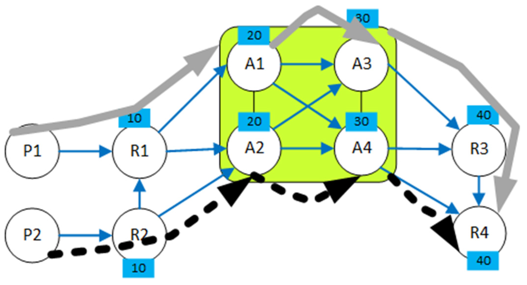
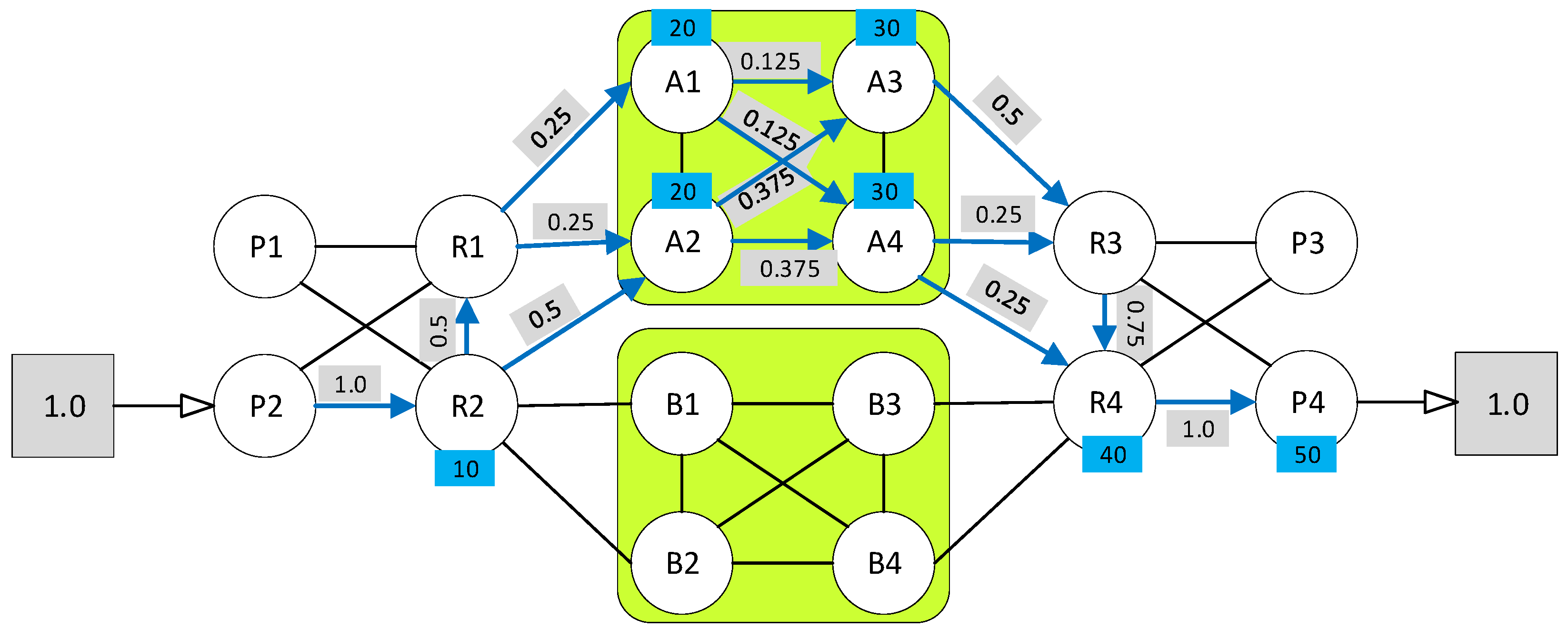
6.1. Phase One: MILP Formulation for EDP
- Input to the optimization problem
- Decision Variables
- Validity and Continuity
- Bandwidth and Length Constraints
- Utilization
- Complete Optimization Formulation
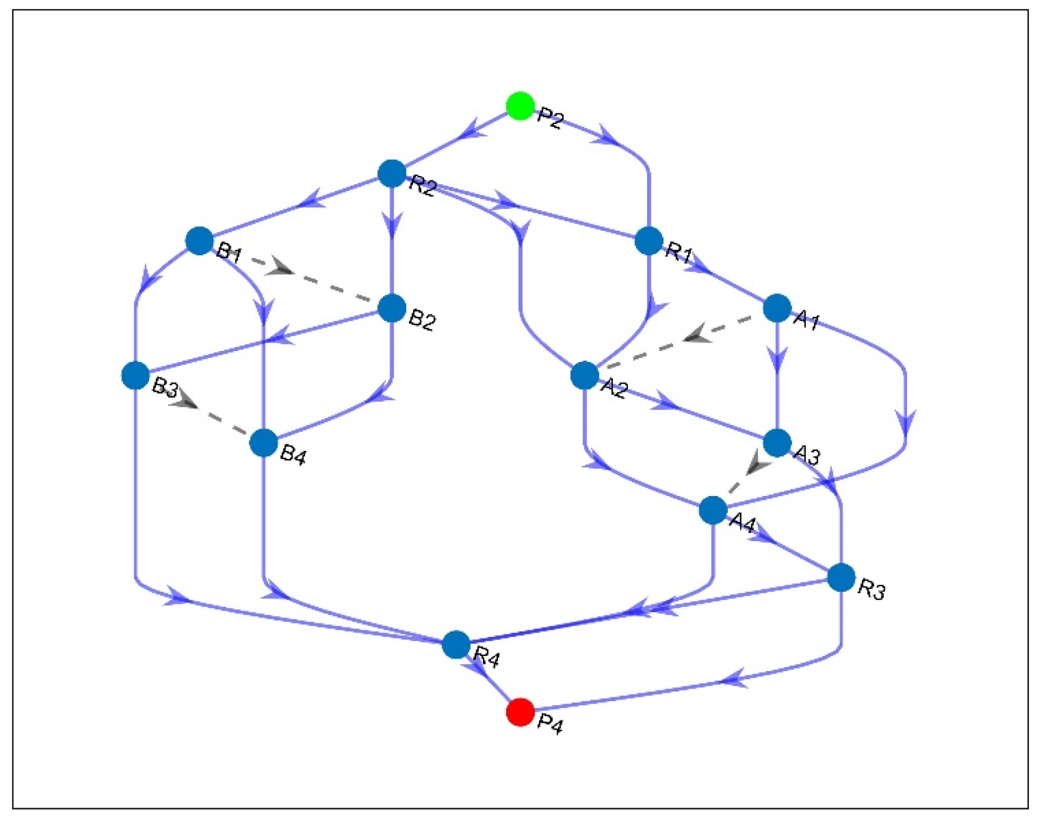
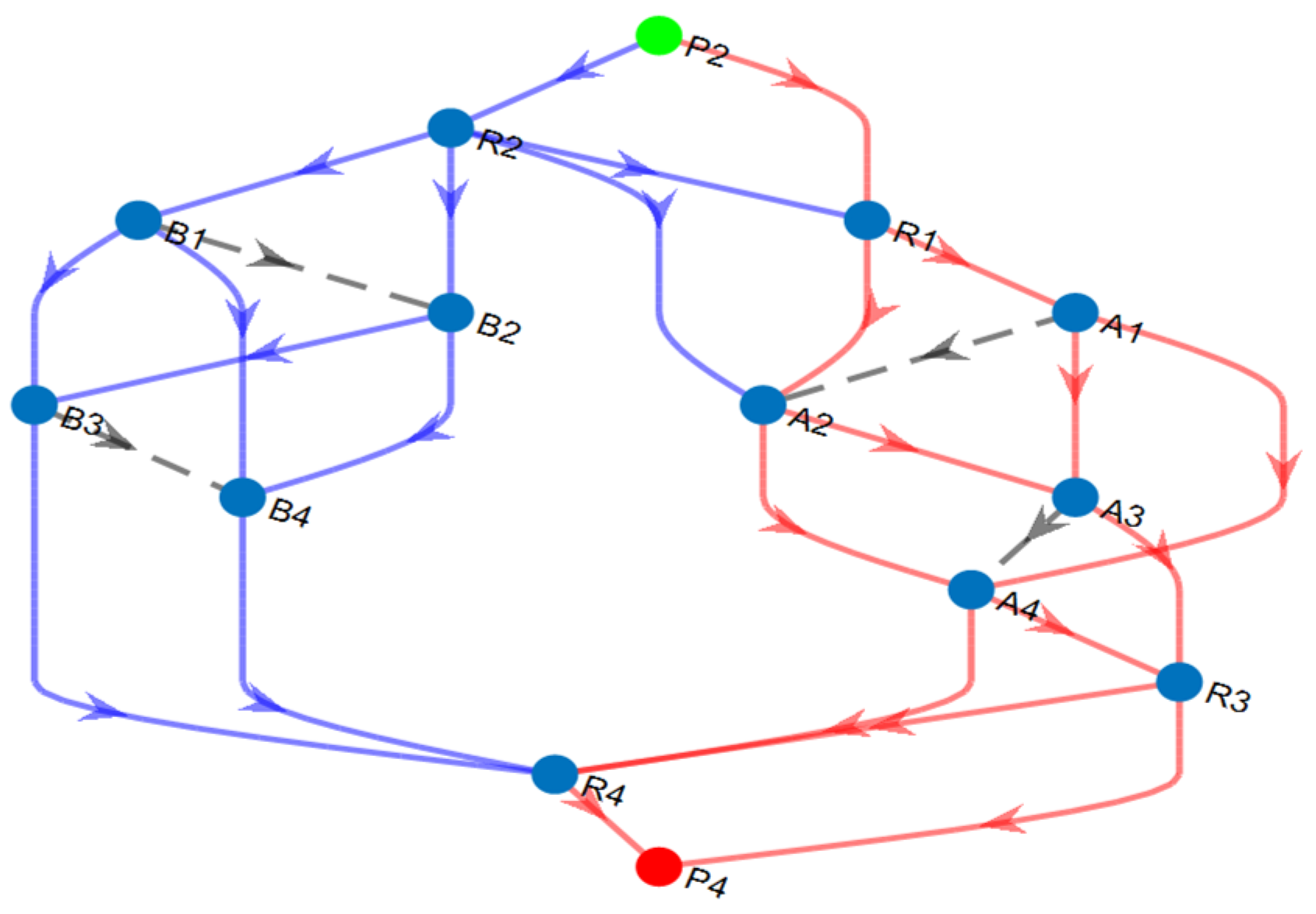
6.2. Phase Two: Finding Working and Backup Multipaths
| Algorithm 1: Link Distribution and Conflict Resolution (LDCR) |
| Input: single multipath from phase one, src, and des. |
| Output: two disjoint multipaths: working and backup |
|
- E-LDCR Methodology
6.3. Qualitative Analysis of the Working and Backup Sets
6.3.1. The Edge-Cut Set: Revisited
6.3.2. The Influence Measure
6.3.3. Path Operational Probability
7. Experimental Results
7.1. Validation
7.2. Effectiveness
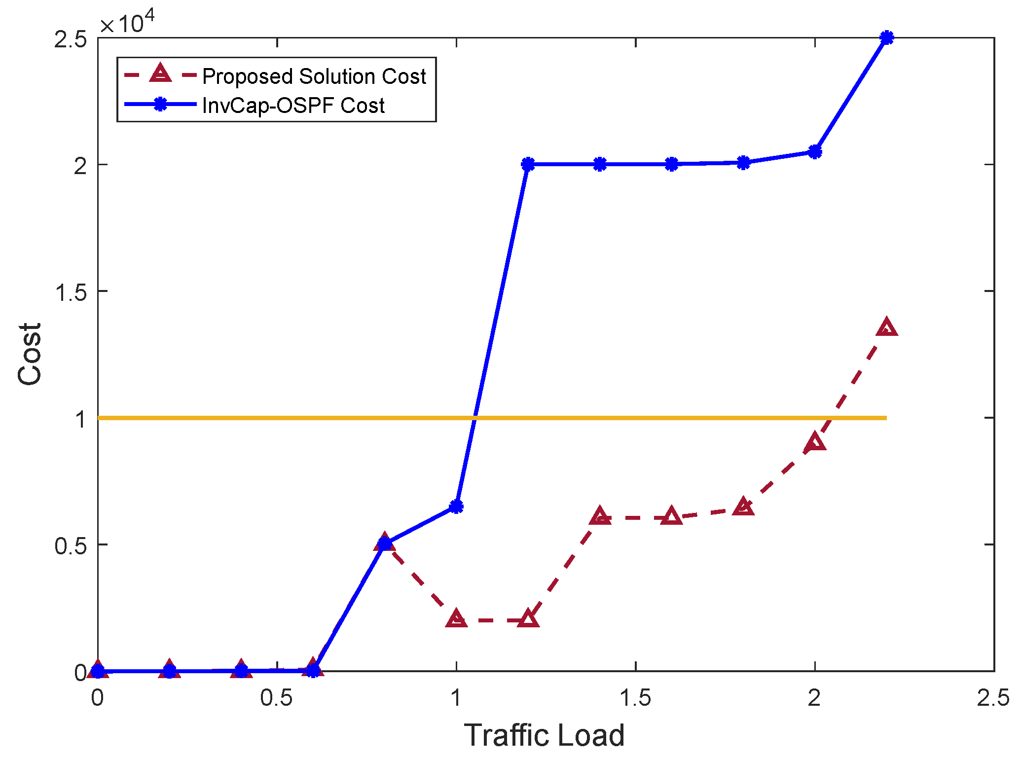
7.2.1. Networkwide Cost Function
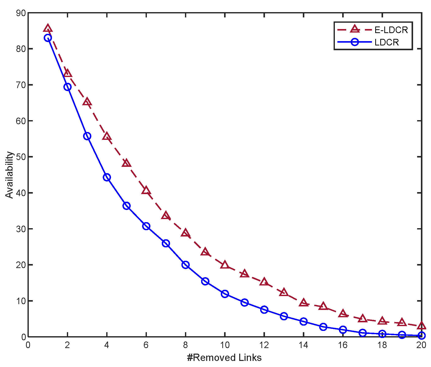
7.2.2. Network Availability
7.2.3. Max-Utilization Performance Evaluation
7.3. Evaluating the Quality of Working and Backup Multipaths
7.3.1. Operational Probability
7.3.2. Graph-Related Metrics
8. Conclusions
Funding
Data Availability Statement
Conflicts of Interest
References
- Tian, Y.; Wang, Z.; Yin, X.; Shi, X.; Guo, Y.; Geng, H.; Yang, J. Traffic Engineering in Partially Deployed Segment Routing over IPv6 Network with Deep Reinforcement Learning. IEEE/ACM Trans. Netw. 2020, 28, 1573–1586. [Google Scholar] [CrossRef]
- Zeng, R.; You, J.; Li, Y.; Han, R. An ICN-Based IPFS High-Availability Architecture. Future Internet 2022, 14, 122. [Google Scholar] [CrossRef]
- Wang, L. Architecture-Based Reliability-Sensitive Criticality Measure for Fault-Tolerance Cloud Applications. IEEE Trans. Parallel Distrib. Syst. 2019, 30, 2408–2421. [Google Scholar] [CrossRef]
- Di Mauro, M.; Galatro, G.; Longo, M.; Postiglione, F.; Tambasco, M. Comparative Performability Assessment of SFCs: The Case of Containerized IP Multimedia Subsystem. IEEE Trans. Netw. Serv. Manag. 2021, 18, 258–272. [Google Scholar] [CrossRef]
- Bai, J.; Chang, X.; Machida, F.; Jiang, L.; Han, Z.; Trivedi, K.S. Impact of Service Function Aging on the Dependability for MEC Service Function Chain. IEEE Trans. Dependable Secur. Comput. 2022, 20, 2811–2824. [Google Scholar] [CrossRef]
- Egawa, Y.; Kaneko, A.; Matsumoto, M. A mixed version of Menger’s theorem. Combinatorica 1991, 11, 71–74. [Google Scholar] [CrossRef]
- MacDavid, R.; Chen, X.; Rexford, J. Scalable Real-Time Bandwidth Fairness in Switches. In Proceedings of the IEEE International Conference on Computer Communications, New York, NY, USA, 17–20 May 2023. [Google Scholar]
- Hiryanto, L.; Soh, S.; Chin, K.W.; Pham, D.S.; Lazarescu, M. Green Multi-Stage Upgrade for Bundled-Links SDN/OSPF-ECMP Networks. In Proceedings of the IEEE International Conference on Communications, Montreal, QC, Canada, 14–23 June 2021. [Google Scholar] [CrossRef]
- Al Mtawa, Y.; Haque, A.; Sidebottom, G. Disjoint-path Segment Routing: Network: Reliability Perspective. In Proceedings of the 2022 International Wireless Communications and Mobile Computing (IWCMC), Dubrovnik, Croatia, 30 May–3 June 2022; pp. 1076–1081. [Google Scholar] [CrossRef]
- Awad, M.K.; Ahmed, M.H.H.; Almutairi, A.F.; Ahmad, I. Machine Learning-Based Multipath Routing for Software Defined Networks. J. Netw. Syst. Manag. 2021, 29, 18. [Google Scholar] [CrossRef]
- Praveena, H.D.; Srilakshmi, V.; Rajini, S.; Kolluri, R.; Manohar, M. Balancing module in evolutionary optimization and Deep Reinforcement Learning for multi-path selection in Software Defined Networks. Phys. Commun. 2023, 56, 101956. [Google Scholar] [CrossRef]
- Bhardwaj, A.; El-Ocla, H. Multipath routing protocol using genetic algorithm in mobile ad hoc networks. IEEE Access 2020, 8, 177534–177548. [Google Scholar] [CrossRef]
- Srilakshmi, U.; Veeraiah, N.; Alotaibi, Y.; Alghamdi, S.A.; Khalaf, O.I.; Subbayamma, B.V. An improved hybrid secure multipath routing protocol for MANET. IEEE Access 2021, 9, 163043–163053. [Google Scholar] [CrossRef]
- Edmonds, J.; Karp, R.M. Theoretical Improvements in Algorithmic Efficiency for Network Flow Problems. J. ACM 1972, 19, 248–264. [Google Scholar] [CrossRef]
- Yen, J.Y. Finding the K Shortest Loopless Paths in a Network. Manag. Sci. 1971, 17, 712–716. [Google Scholar] [CrossRef]
- Dijkstra, E.W. A note on two problems in connexion with graphs. Numer. Math. 1959, 1, 269–271. [Google Scholar] [CrossRef]
- Martín, B.; Sánchez, Á.; Beltran-Royo, C.; Duarte, A. Solving the edge-disjoint paths problem using a two-stage method. Int. Trans. Oper. Res. 2020, 27, 435–457. [Google Scholar] [CrossRef]
- Pereira, V.; Rocha, M.; Sousa, P. Traffic Engineering with Three-Segments Routing. IEEE Trans. Netw. Serv. Manag. 2020, 17, 1896–1909. [Google Scholar] [CrossRef]
- Li, X.; Yeung, K.L. Traffic Engineering in Segment Routing Networks Using MILP. IEEE Trans. Netw. Serv. Manag. 2020, 17, 1941–1953. [Google Scholar] [CrossRef]
- Dominicini, C.K.; Vassoler, G.L.; Valentim, R.; Villaca, R.S.; Ribeiro, M.R.; Martinello, M.; Zambon, E. KeySFC: Traffic steering using strict source routing for dynamic and efficient network orchestration. Comput. Netw. 2020, 167, 106975. [Google Scholar] [CrossRef]
- Jadin, M.; Aubry, F.; Schaus, P.; Bonaventure, O. CG4SR: Near Optimal Traffic Engineering for Segment Routing with Column Generation. In Proceedings of the IEEE INFOCOM 2019—IEEE Conference on Computer Communications, Paris, France, 29 April–2 May 2019; Institute of Electrical and Electronics Engineers Inc.: Piscataway, NJ, USA, 2019; pp. 1333–1341. [Google Scholar] [CrossRef]
- Suurballe, J.W. Disjoint paths in a network. Networks 1974, 4, 125–145. [Google Scholar] [CrossRef]
- Suurballe, J.W.; Tarjan, R.E. A quick method for finding shortest pairs of disjoint paths. Networks 1984, 14, 325–336. [Google Scholar] [CrossRef]
- Fortz, B.; Thorup, M. Internet traffic engineering by optimizing OSPF weights. In Proceedings of the IEEE INFOCOM 2000 Conference on Computer Communications. Nineteenth Annual Joint Conference of the IEEE Computer and Communications Societies (Cat. No.00CH37064), Tel Aviv, Israel, 26–30 March 2000; pp. 519–528. [Google Scholar] [CrossRef]


| Links of Conflict (Index, Name) | Conflicting Working Paths (Path Index) | Conflicting Backup Paths (Path Index) |
|---|---|---|
| 7, (R1, A2) | 1 | 1, 2 |
| 8, (R1, A1) | 2 | 3, 4 |
| 11, (A2, A4) | 1, 3 | 2 |
| 13, (A1, A4) | 2 | 4 |
| Path Index | Path | |
|---|---|---|
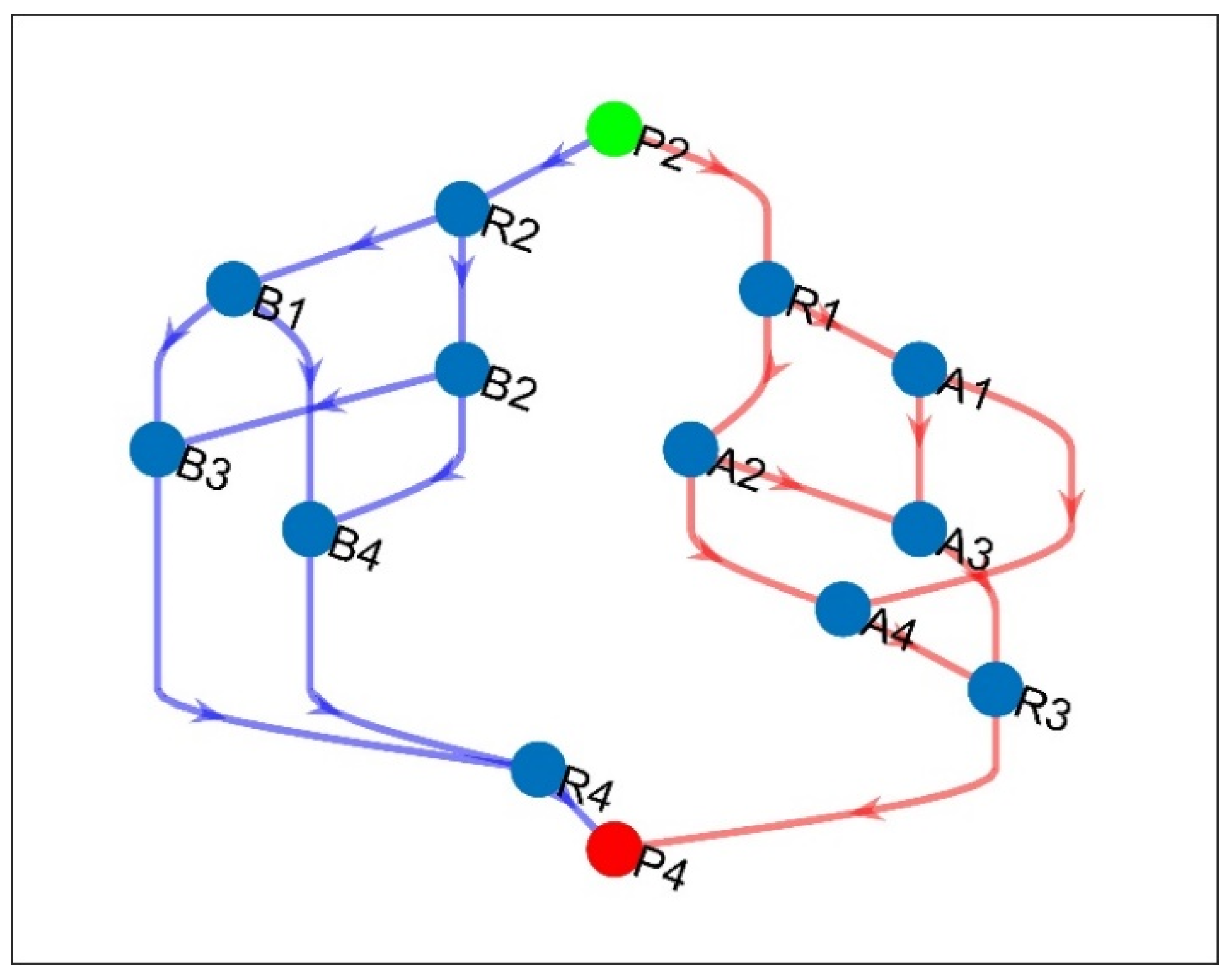
| Working | 1 | P2—R2—R1—A2—A4—R4—P4 |
| 2 | P2—R2—R1—A1—A4—R4—P4 | |
| 3 | P2—R2—A2–A4—R4—P4 | |
| Backup | 1 | P2—R1—A2—A3—R3—P4 |
| 2 | P2—R1—A2—A4—R3—P4 | |
| 3 | P2—R1—A1—A3—R3—P4 | |
| 4 | P2—R1—A1—A4—R3—P4 | |
| Variable/Path Removal | |||||
|---|---|---|---|---|---|
| (R1, A2) | W-1 | 1 | 1 | 2 | 3 |
| B-1,2 | 2 | 2 | 2 | 2 | |
| (R1, A1) | W-2 | 2 | 1 | 2 | 4 |
| B-3,4 | 2 | 2 | 1 | 1.5 | |
| (A2, A4) | W-1,3 | 2 | 2 | 2 | 2 |
| B-2 | 1 | 1 | 2 | 3 | |
| (A1, A4) | W-2 | 2 | 1 | 2 | 4 |
| B-4 | 1 | 1 | 1 | 2 | |
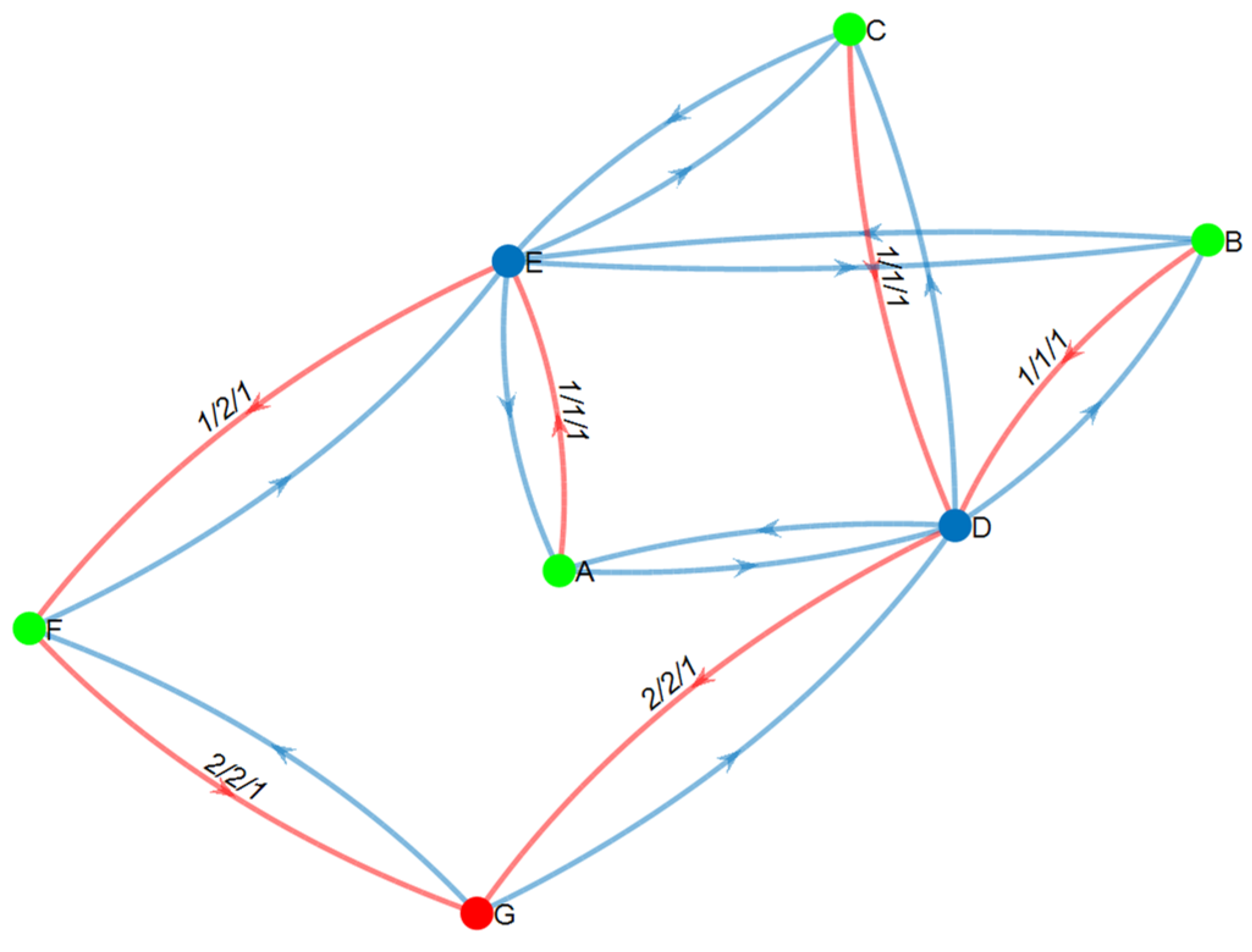
| Multipaths | Operational Probability | Normalized Operational Probability | Probability of Using Backup Multipath if the Working Is Failed | |
|---|---|---|---|---|
| Working | ABEH | 0.75 | 0.18 | |
| ABH | 0.87 | 0.20 | ||
| ACGH | 0.87 | 0.20 | ||
| Backup | ADFH | 0.86 | 0.20 | 0.0039 + 0.0041 = 0.008 |
| ADH | 0.92 | 0.22 | ||
| Metric | Working | Backup |
|---|---|---|
| 2 | 1.75 | |
| for C, G, and E for B | for D for F |
Disclaimer/Publisher’s Note: The statements, opinions and data contained in all publications are solely those of the individual author(s) and contributor(s) and not of MDPI and/or the editor(s). MDPI and/or the editor(s) disclaim responsibility for any injury to people or property resulting from any ideas, methods, instructions or products referred to in the content. |
© 2023 by the author. Licensee MDPI, Basel, Switzerland. This article is an open access article distributed under the terms and conditions of the Creative Commons Attribution (CC BY) license (https://creativecommons.org/licenses/by/4.0/).
Share and Cite
Al Mtawa, Y. Enhancing Network Availability: An Optimization Approach. Computation 2023, 11, 202. https://doi.org/10.3390/computation11100202
Al Mtawa Y. Enhancing Network Availability: An Optimization Approach. Computation. 2023; 11(10):202. https://doi.org/10.3390/computation11100202
Chicago/Turabian StyleAl Mtawa, Yaser. 2023. "Enhancing Network Availability: An Optimization Approach" Computation 11, no. 10: 202. https://doi.org/10.3390/computation11100202
APA StyleAl Mtawa, Y. (2023). Enhancing Network Availability: An Optimization Approach. Computation, 11(10), 202. https://doi.org/10.3390/computation11100202