1. Introduction
With the expected increase in world energy demand, access to reliable energy at affordable prices is essential for economic and social well-being and is an important development indicator. At the same time, energy production lies at the root of the pollution and greenhouse gas emissions that contribute decisively to climate change. Thus, the fight against climate change and the reduction in greenhouse gas emissions became a central issue on the agendas of practically all countries in the world, with issues related to energy sources and energy efficiency fundamental to this cause. Kabouris and Kanellos [
1] present significant technical challenges posed by the integration of renewable energy mainly due to its variable and hard-to-predict nature.
Currently, around 85% of the world’s primary energy consumption comes from non-renewable energy sources, with renewable sources representing only 15%, and of these, wind energy represents 2.1% [
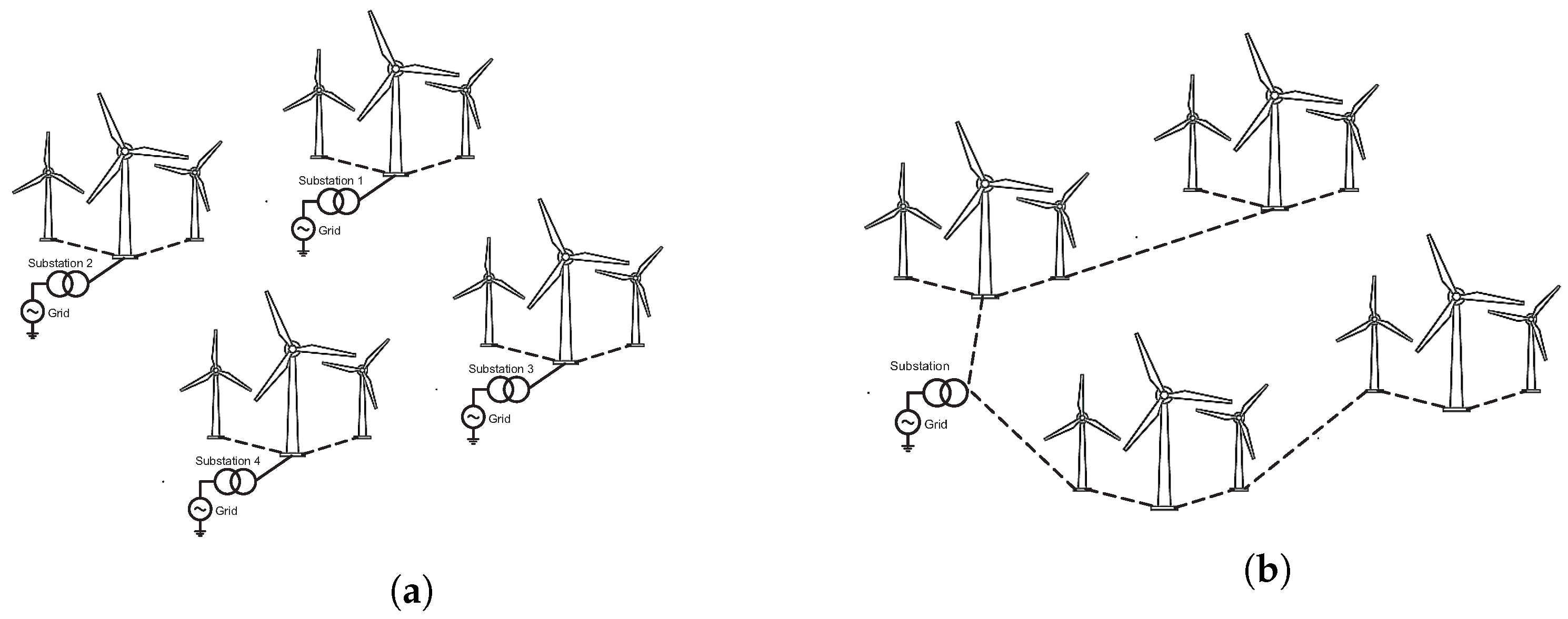
2]. Therefore, there is still a long way to go, which involves continuous renewable energy investments, particularly onshore and offshore wind power. The vast majority of medium and large wind farms are constituted of several dozen wind turbines dispersed by agglomerates that can be connected to one or more substations regarding onshore wind farms. In this type of situation, the technical solutions found on the ground to interconnect all turbines and substations can be diverse, resulting in different costs of installing the distribution network and different values for energy losses.
Optimizing the wind farm distribution grid is crucial for several reasons, and it contributes to the overall efficiency, reliability, and economic viability of the wind energy system. The best optimization solutions can maximize energy production, extracting the maximum amount of energy from wind resources. The grid’s stability and reliability can be enhanced, and efficiency improvements resulting from optimization can lead to cost savings. This includes better maintenance planning, reduced downtime, and increased lifespan of equipment. Additionally, optimized energy production can contribute to a more cost-effective energy generation process. Many regions have regulations and standards in place to ensure the stability and reliability of the power grid. Optimizing the wind farm power grid helps meet these regulatory requirements, avoiding penalties and ensuring compliance. In summary, optimizing the power grid of a wind farm is essential for maximizing energy production, ensuring grid stability, reducing costs, meeting regulatory requirements, and advancing the overall sustainability and reliability of the energy system.
Most of the works found in the literature consider wind farms with only one substation and optimize the cable layout to interconnect the turbines to the substation, using exact methods [
3,
4,
5,
6,
7,
8,
9,
10,
11] or meta-heuristics [
12,
13,
14,
15,
16,
17]. On the other hand, when several substations are taken into account, the topology connection (identify the substation at which the turbines are connected) and the cable connection (connection layout between turbines and its substation) designs are considered separately, leading to suboptimal solutions. The last kind of work is described in the following.
Fischetti and Pisinger [
18] combine mixed-integer linear programming with math-heuristics to optimize the cable connections of wind farms. The problem was modeled to consider more than one substation. However, the MILP model only manages to solve the smallest problems in a reasonable time. Since the instances were not clearly described in the work, it is not possible to know if the results consider windfarms with more than one substation.
In [
19], the authors propose an integer linear programming model for the design of wind farms with multiple substations, minimizing the costs of infrastructure and energy losses. Moreover, considering a discrete set of possible turbine locations, the model is able to identify those that should be present in the optimal solution, hence addressing the optimal location of the substation(s) in the wind farm.
Srikakulapu and U [
20] minimize the investment cost and power losses in the cable connections of wind farms using a three-step algorithm: wind turbines allocation, where the turbines are grouped using a fuzzy clustering algorithm; wind turbines reallocation, where the turbines are allocated to their nearest substations using a binary programming model; cable layout optimization, where a minimum spanning tree algorithm is used to minimize the total length layout design for wind farm cable connections. Considered separately, the allocation turbines and the optimization layout length could lead to a suboptimal solution. They present results for a wind farm with three substations and 50 turbines. Zuo et al. [
21] use a fuzzy clustering technique to determine the substation locations and the minimum spanning tree model to find the cable connection layout for offshore wind farms’ re-powering and expansion.
Dutta and Overbye [
22] use a clustering algorithm to determine the cable layout for wind farms. In this work, the authors claim that the proposed method yielded lower collector system real power losses when compared to the conventional radial or daisy chain cable layout method.
Wu and Wang [
23] use the k-means clustering and ant colony algorithm to reduce wind farms’ construction costs and the collector system’s reliability. They present a problem with four substations, using the clustering algorithm to assign the turbines to a substation.
Wang et al. [
24] present an integrated design method for wind farms, considering the substation location, connection topology, and cable cross-sections to minimize the total cost. They use an evolutionary algorithm to solve the problem. Moreover, they use a heuristic algorithm to find the substation coordinates, the substation associated with each turbine, and the cable layout. The authors consider only wind farms with one and two substations with 56 and 40 turbines, respectively.
Pillai [
25] proposes an approach for a cable design of a wind farm. They divide the problem into some subproblems, each one with one substation. The substation places are determined via the proposed approach, where a capacitated clustering approach for placing the substations is used. On the other hand, a mixed-integer linear program (MILP) to solve each subproblem and determine the cable connection and cable type to be installed is used. The MILP uses some initial solutions obtained via heuristics.
This paper’s main contribution is to optimize the layout of wind farms, in one step, considering multiple substations and cable connections, in contrast to the usual approaches found in the literature, which address only one singular substation or a reduced number of turbines. In the optimization process, a genetic algorithm is used to determine the topology design, and an integer linear programming model determines the optimal cable connection. The overall objective function minimizes energy losses and cable installation costs. The case studies presented consider up to five substations and 120 wind turbines, but the methodology could be extended to higher dimensions.
Wind farms with several substations result in lower power transformers’ installation and consequently, lower insulation levels in all protection equipment, which increases the efficiency of the WF, resulting in higher profitability by improving the LCOE (Levelized Cost of Electricity).
The remaining part of the paper is divided into the following.
Section 2 describes the electrical power grid to model the wind farm problem.
Section 3 characterizes briefly the wind farms considered in the study and the adopted methodology to solve the layout problem.
Section 4 describes how the turbines’ assignment to the substations was addressed and the cable connections were determined.
Section 5 presents the obtained results and discusses them. Finally,
Section 6 draws the main conclusions.
2. Electrical Power Grid Modeling
The selection of the structure of a wind farm is a process that involves multidisciplinary teams (engineering, economy, environment, and even evaluation of social impacts), with different objectives but always in search of a common goal that goes through the optimization of the whole structure harmoniously.
A wind farm consists of three blocks, the energy collection system, the integration system, and the transmission system. The first one is responsible for collecting the wind turbines’ energy and routing it to the main substation. In the case of large wind farms, there may be an arrangement in clusters, each with a substation interconnected through a distribution network to the main substation. The second block is responsible for integrating all the elements, optimally allowing the energy produced to be routed to the substations, which is usually performed with voltage levels of 20/30 kV. The transmission system is responsible for injecting the produced energy into the transmission network, which is generally conducted at high voltage, for example, 150 kV.
In the wind farm distribution network, where each node represents a wind turbine, to carry out a stationary analysis of the power flow, it is essential to know all the network parameters to develop a model for all of them. These networks have a radial structure, and it is necessary to understand how to calculate the transit of energy flowing there. Some work in the literature deals precisely with the problem of power transit in radial networks [
26,
27,
28,
29]. In addition, works such as [
30] are dedicated to the reactive energy optimization problem in radial networks, presenting contributions in calculating load flow and adapting to these networks’ radial characters.
In this paper’s study, which has as the main objective the optimization of the cable layout considering several substations in wind farms, as shown in
Figure 1, it is essential to know the parameters associated with the internal distribution network.
As referenced by Cerveira et al. [
4], in wind farms’ distribution networks, the short line model should be used. This choice is because the networks that connect the various elements of a wind farm are lower than a few kilometers, where the R/X ratio is high. With the short line model, several simplifications can be made, and the cables’ shunt admittance can be neglected. Therefore, the network branches can be represented by the model of
Figure 2. Moreover, a radial cable network structure is considered where Kirchoff’s current and voltage laws and the branch current stability constraint are guaranteed.
The load constraints considered in this study are power balance constraints described by a set of power flow equations for balanced radial distribution networks developed in [
31]. Therefore, the power flowing at the receiving end of the branch
,
,
, and the voltage magnitude at the sending end
can be expressed via Equations (
1)–(
3).
where
and
represent the active and reactive power, respectively, leaving the sending bus
n, while
and
are the active and reactive power that flow on the bus
n, regarding the wind farm branches connected to that bus, and
is the voltage at bus
n. The branch resistance and reactance between buses
n and
are represented by
and
, respectively.
It should be noted that the voltage drop between any two buses should be within regulatory limits, which may be up to 5% of the network voltage, U. The model considered here does not include those constraints that are naturally guaranteed in the solutions by the dimensions of the case studies discussed.
To obtain the branch losses between the bus
n and bus
, Equations (
4)–(
6) are used:
Therefore, the total power losses,
, can then be obtained by adding the losses from all cable connections, as given by
where
N is the set of the nodes in the network.
The values of
and
depend on the cable used. In this work, a set of cable types, presented in
Table 1, is considered. Each cable type
k is characterized by its section, an inductance
per unit of length, a resistance
per unit of length, a maximum current intensity
that it can support, and a cost
per unit of length.
The maximum current intensity,
, bounds the number of wind turbines in any branch line, i.e., in a set of connections starting with a direct link to the substation. Furthermore, it will determine the types of cable that could be used depending on the number of downstream wind turbines. It should be noted that the rated current drawn by each turbine, defined by
, is given by
where
is the rated power of the wind turbines and
U is the interconnection grid’s voltage. The value of
is the turbine’s power factor, and, in the case studies, it is considered that the current and voltage drop drawn into the network are in phase, i.e.,
. In each wind farm, with a particular value of
U and
, the
value restricts the cable type that can be used in a connection depending on the number of downstream wind turbines.
To exemplify this, consider the wind farm layout presented in
Figure 3, with one substation, node 0, and eight wind turbines, nodes 1 to 8. In this example, assuming that
MW and
kV, the rated current drawn by each turbine is
A (via Equation (
8)). This layout has two branch lines: one starting in cable connection
with blue wind turbines and the other starting in cable connection
with red wind turbines. The total current reaching the substation from a branch line is the sum of the currents drawn by all turbines connected through this branch. For instance, the branch starting in connection
supports five wind turbines (including turbine 2). Therefore, the current passing through this cable is
A. Given that, this connection cannot use a cable of type less than five which has
. Furthermore, in a wind farm with
and
U values, any branch line cannot have more than
wind turbines, where
denotes the maximum integer not greater than
a.
5. Results and Discussion of the Case Studies
This section presents and discusses the results using the proposed methodology. The GA was written in Python, and the fitness function requires solving the integer programming model Layout+. The integer programming models are solved using the Xpress optimizer library.
Table 2 sums up the GA parameters used, which were chosen based on computational experiments.
The proposed methodology was applied to four wind farms, with two, three, four, and five substations. The first wind farm is the
Alto da Coutada wind farm, located in the north of Portugal, formed of 79 turbines and two substations. The second wind farm, called WF-S3, is formed of 74 turbines and three substations, generated according to an example in [
40]. The third wind farm, called WF-S4, has four substations and 79 turbines. The last wind farm is the
Alto Minho, located in the north of Portugal, formed of 120 turbines and five substations.
In all case studies, the following were considered: ten cable types presented in
Table 1,
EUR/Wh as the energy cost,
as the number of hours during the expected lifetime of the wind farm (20 years ),
as the load factor, and
rad/s as the angular frequency.
5.1. Alto da Coutada Wind Farm
The first case study is the Alto da Coutada wind farm with two substations and 50 wind turbines with
MW of rated power, interconnected by a
kV grid. With these parameters, the rated current drawn by each turbine is
A, and the maximum number of wind turbines per branch line is
. The coordinates of the wind turbines are in [
4], and the coordinates of the two substations are {(41.5227550, −7.5958050), (41.5792210, −7.5358600)}.
The obtained cable connection layout is presented in
Figure 6. The wind farm has two wind fields (a parcel of a wind farm with one substation),
and
, where the turbine sets linked to substations
and
are, respectively,
{1, 2, 3, 4, 5, 6, 7, 8, 9, 10, 11, 12, 13, 14, 15} and
{16, 17, 18, 19, 20, 21, 22, 23, 24, 25, 26, 27, 28, 29, 30, 31, 32, 33, 34, 35, 36, 37, 38, 39, 40, 41, 42, 43, 44, 45, 46, 47, 48, 49, 50}. On each wind field, the turbines are filled with the same color.
Table 3 shows the connections and their cable type for each wind field in the final solution and the corresponding costs. The first column presents the substation,
, and the number of turbines assigned to it,
. The next three columns, “
k”, “Links”, and “#Links”, indicate the type of cables used, the links
of this cable type, and the corresponding number of cables, in the solution. Finally, the column “Cost” presents the global total cost
f of the wind farm, the total cost
of the wind fields
, and the partial cost of each wind field, namely, infrastructure cost
, active losses
, and reactive losses
.
The total cost layout of the two wind fields is EUR 4,795,930.7. The wind field has 15 wind turbines, and the total cost is EUR 1,239,980.2, where 55.7% is the infrastructure cost, corresponding to EUR 690,802.4, 24.1% is the active losses cost, corresponding to EUR 298,316.2, and 20.2% is the reactive losses cost, corresponding to EUR 25,0861.6. The wind field has 35 wind turbines, and its total cost is EUR 3,555,951.7, where 54.7% is the infrastructure cost, 23.9% is the active losses cost, and the remaining 21.4% is the reactive losses cost. The highest amount corresponds to the infrastructure cost, and the smallest cost is the reactive losses cost during the wind farm lifetime.
The clustering algorithm is used to infer the GA’s performance. The turbines are first assigned to the closest substation via the clustering algorithm, followed by the ILP model, Layout+, to optimize the wind farm layout considering the WT assignments. The obtained solution is then compared with the one obtained in the previous section. The turbine sets assigned to substations
and
are, respectively,
{1, 2, 3, 4, 5, 6, 7, 8, 9, 10, 11, 12, 13} and
{14, 15, 16, 17, 18, 19, 20, 21, 22, 23, 24, 25, 26, 27, 28, 29, 30, 31, 32, 33, 34, 35, 36, 37, 38, 39, 40, 41, 42, 43, 44, 45, 46, 47, 48, 49, 50}. The obtained objective value corresponds to the cost EUR 4,800,839.0. This value is higher than the one obtained via the GA. It can be observed that, in the solution presented in
Section 5.1, turbines 14 and 15 are not assigned to the nearest substation,
. Thus, it can be concluded that the clustering algorithm could lead to a worse solution than the one obtained with the proposed methodology. In
Figure 6, turbines grouped differently in the two algorithms are highlighted using different colors for the labels. Turbines with different label colors mean that the turbine is connected to another substation (according to its color) in the clustering algorithm.
5.2. WF-S3 Wind Farm
The second case study is the WF-S3 wind farm with three substations and 74 wind turbines with
MW of rated power, interconnected by a
kV grid. With these parameters, the rated current drawn by each turbine is
A, and the maximum number of wind turbines per branch line is
. The coordinates of the wind turbines and substations are in
Table A1.
The obtained cable connection layout is presented in
Figure 7. The wind farm has three wind fields,
,
, and
, where the turbine sets linked to substations
,
, and
are, respectively,
{1, 2, 3, 4, 5, 6, 7, 8, 9, 10, 14, 17, 19, 20, 21, 22, 23, 24},
{18, 25, 26, 27, 28, 29, 30, 31, 32, 33, 34, 35, 36, 37, 38, 39, 40, 41, 42, 43, 44, 45, 46, 47, 48, 49}, and
{11, 12, 13, 15, 16, 50, 51, 52, 53, 54, 55, 56, 57, 58, 59, 60, 61, 62, 63, 64, 65, 66, 67, 68, 69, 70, 71, 72, 73, 74}. In the presented solution, it can be observed that some border turbines are not assigned to the nearest substation.
Table 4 characterizes the connections and costs for each wind field in the final solution. The total cost layout of the three wind fields is EUR 2,838,121.1. The wind field
has 18 wind turbines, and the total cost is EUR 658,709.8, where 70.4% is the infrastructure cost, corresponding to EUR 463,373.1, 19.2% is the active losses cost, corresponding to EUR 126,267.6, and 10.5% is the reactive losses cost, corresponding to EUR 69,069.1. The wind field
has 26 wind turbines. Its total cost is EUR 1,036,720.7, where 64.0% is the infrastructure cost, 22.6% is the active losses cost, and the remaining 13.4% is the reactive losses cost. The wind field
has 30 wind turbines, and the total cost is EUR 1,142,690.6, where 64.9% is the infrastructure cost, 22.8% is the active losses cost, and the remaining 12.3% is the reactive losses cost. Again, the higher cost is the infrastructure and the lower cost is the cost of reactive losses over the lifetime of the wind farm.
To complete the proposed approach’s performance analysis, we will present the solution using a clustering algorithm to assign turbines to the closest substation, instead of the GA, followed by the ILP model, Layout+. The turbine sets assigned to substations , , and are, respectively, {1, 2, 3, 4, 5, 6, 7, 8, 9, 10, 14, 15, 17, 19, 20, 21, 22, 23, 24}, {18, 25, 26, 27, 28, 29, 30, 31, 32, 33, 34, 35, 36, 37, 38, 39, 40, 41, 42, 43, 44, 45, 46, 47, 48, 49}, and {11, 12, 13, 16, 50, 51, 52, 53, 54, 55, 56, 57, 58, 59, 60, 61, 62, 63, 64, 65, 66, 67, 68, 69, 70, 71, 72, 73, 74}. The obtained objective value corresponds to the cost EUR 2,839,945.3. This value is higher than the one obtained via the GA. Indeed, for turbine 15, although it is closer to substation 0, the connection of it to substation 0 leads to a cheaper solution.
5.3. WF-S4 Wind Farm
The third case study is the WF-S4 wind farm with four substations and 79 wind turbines with
MW of rated power, interconnected by a
kV grid. With these parameters, the rated current drawn by each turbine is
A, and the maximum number of wind turbines per branch line is
. The coordinates of the wind turbines and substations are in
Table A2.
The obtained cable connection layout is presented in
Figure 8. The wind farm has four wind fields,
,
,
, and
, where the turbine sets linked to substations
,
,
, and
are, respectively,
{3, 4, 5, 6, 7, 13, 14, 15, 16, 22, 23, 24, 32, 33, 34},
{40, 44, 45, 46, 50, 51, 52, 57, 58, 59, 60, 61, 62, 68, 69, 70, 71, 72, 73, 77},
{1, 2, 11, 12, 21, 26, 27, 28, 29, 30, 31, 38, 39, 42, 43, 49, 55, 56, 65, 66, 67, 75, 76}, and
{8, 9, 10, 17, 18, 19, 20, 25, 35, 36, 37, 41, 47, 48, 53, 54, 63, 64, 74, 78, 79}.
Table 5 shows the connections and cable type presented in the final solution and the corresponding costs for each wind field.
The total cost layout of the four wind fields is EUR 7,159,067.8. The wind field has 15 wind turbines, and the total cost is EUR 1,217,848.0, where 63.3% is the infrastructure cost, corresponding to EUR 771,301.4, 23.8% is the active losses cost, corresponding to EUR 289,847.9, and 12.9% is the reactive losses cost, corresponding to EUR 156,698.7. The wind field has 20 wind turbines, and the total cost is EUR 1,760,766.6, where 61.9% is the infrastructure cost, 22.3% is the active losses cost, and the remaining 15.8% is the reactive losses cost. Wind field has 23 wind turbines, and the total cost is EUR 2,080,631.6, where 62.3% is the infrastructure cost, 24.1% is the active losses cost, and 13.6% is the reactive losses cost. The wind field has 21 wind turbines, and the total cost is EUR 2,099,821.7, with EUR 1,297,584.1 for the infrastructure cost, EUR 466,272.4 for the active losses cost, and EUR 335,965.2 for the reactive losses cost.
The WT-S4 wind farm results where the turbines were first assigned to the closest substation via a clustering algorithm followed by the ILP model Layout+ are presented in the following. The turbine sets assigned to substations , , , and are, respectively, {3, 4, 5, 6, 7, 8, 13, 14, 15, 16, 22, 23, 24, 32, 33, 34, 40}, {44, 45, 46, 50, 51, 52, 57, 58, 59, 60, 61, 62, 68, 69, 70, 71, 72, 77}, {1, 2, 11, 12, 21, 26, 27, 28, 29, 30, 31, 38, 39, 42, 43, 49, 55, 56, 65, 66, 67, 75, 76}, and {9, 10, 17, 18, 19, 20, 25, 35, 36, 37, 41, 47, 48, 53, 54, 63, 64, 73, 74, 78, 79}. The obtained objective value corresponds to the cost EUR 7,170,952.23. This value is higher than the one obtained via the GA. Although turbines 8 and 40 are closer to substation 0 and turbine 73 is closer to substation 0, a cheaper solution is obtained if they are connected to substations 0 and 0, respectively.
5.4. Alto Minho Wind Farm
The last case study is the
Alto Minho wind farm, with five substations and 120 turbines. This wind farm spans four locations, namely,
Picos,
São Silvestre,
Santo António, and
Mendoiro.
Santo António has two substations and the others have one each.
Picos has 26 turbines,
São Silvestre has 19 turbines,
Santo António has 61 and 33 (94), and
Mendoiro 26. So, the park is divided into five well-defined regions. Therefore, it is easy to determine the turbine set assigned to each substation. However, the GA is used to solve the problem to validate the algorithm. The results obtained are depicted in
Figure 9, where each wind field
is illustrated with different colors.
Figure 9a shows all the regions, the black circles point out the substations, and the other colored circles indicate the turbines. It can be easily seen that the GA divides the turbines well over the fields.
Figure 9b zooms in on the
Picos wind field, and
Figure 9c zooms in on the
São Silvestre wind field,
Figure 9d zooms in on the
Mendoiro wind field.
Figure 9e zooms in on the
Santo António I wind field, and finally,
Figure 9f zooms in on the
Santo António II wind field.
The turbine sets linked to substations , , , , and are, respectively, {1, 2, 3, 4, 5, 6, 7, 8, 9, 10, 12, 13, 14, 18, 19, 20, 21, 22, 23, 24, 25, 26}, {27, 28, 29, 30, 31, 32, 33, 34, 35, 36, 37, 38, 39, 40, 41, 42, 43, 44, 45}, {46, 47, 48, 49, 50, 51, 52, 53, 54, 55, 56, 57, 58, 59, 60, 61}, {62, 63, 64, 65, 66, 67, 68, 69, 70, 71, 72, 73, 74, 75, 76,77, 78, 79, 80, 81, 82, 83, 84, 85, 86, 87, 88, 89, 90, 91, 92, 93, 94}, and {95, 96, 97, 98, 99, 100, 101, 102, 103, 104, 105, 106, 107, 108, 109, 110, 111, 112, 113, 114, 115, 116, 117, 118, 119, 120}.
Table 6 shows the connections and cable type presented in the final solution and the corresponding costs for each wind field.
The total cost layout of the five wind fields is EUR 5,439,809.2. The wind field has 26 wind turbines, and the total cost is EUR 1,255,170.5, where 57.0% is the infrastructure cost, corresponding to EUR 715,716.4, 23.6% is the active losses cost, corresponding to EUR 296,430.9, and 19.4% is the reactive losses cost, corresponding to EUR 243,023.2. The wind field has 19 wind turbines, and the total cost is EUR 873,066.6, where 57.8% is the infrastructure cost, 23.1% is the active losses cost, and the remaining 19.2% is the reactive losses cost. The wind field has 16 wind turbines, and the total cost is EUR 595,478.1, where 58.1% is the infrastructure cost, 23.5% is the active losses cost, and 18.4% is the reactive losses cost. The wind field has 38 wind turbines, and the total cost is EUR 1,304,863.9, with EUR 758,211.4 for the infrastructure cost, EUR 305,002.4 for the active losses cost, and EUR 241,650.1 for the reactive losses cost. The wind field has 26 wind turbines and the total cost is EUR 1,411,230.1, with the infrastructure cost contributing 57.2% (EUR 807,677.4), the active losses 23.8% (EUR 336,226.6), and the reactive losses cost 18.9% (EUR 267,326.1).
The most expensive wind field is , although it has 12 fewer turbines than . This fact is due to the position of substation 0, which is more central and has more turbines nearby.
In all case studies, the solutions only present cables of type .
The Alto Minho wind farm results where the turbines were first assigned to the closest substation via the clustering algorithm followed by the ILP model, Layout+, are the same as the GA results. This fact is because turbines are grouped closest to one substation and very far from the others.
5.5. Genetic Algorithm versus Clustering Algorithm
This section summarizes the optimization results of previous sections, comparing the two approaches, GA and clustering.
Table 7 presents the optimal fitness values and total costs of the solutions for the GA and clustering algorithms in lines “GA” and “Clustering”, respectively. It can be observed that the GA obtains better results than the clustering algorithm in the first three wind farms and the same outcome in the last wind farm.
For each wind farm, the GA ran five times, and in all executions, the GA found the same solution.
Table 7 also illustrates the minimum, maximum, median, mean, and standard deviation of the number of iterations needed by the GA to reach the final solution. It could be observed that the algorithm needs a small number of iterations to obtain the final solution. In addition, the GA approach achieves up to
of economic savings compared to the clustering approach.
The proposed method optimizes the problems in a single phase, allowing the method to converge to the global optimum. In contrast, sequential optimization does not avoid the convergence to local optima that often occurs. This phenomenon was observed using the clustering technique, when the turbines were grouped to a substation in the first phase and the connections to the substation were optimized in the second phase.


