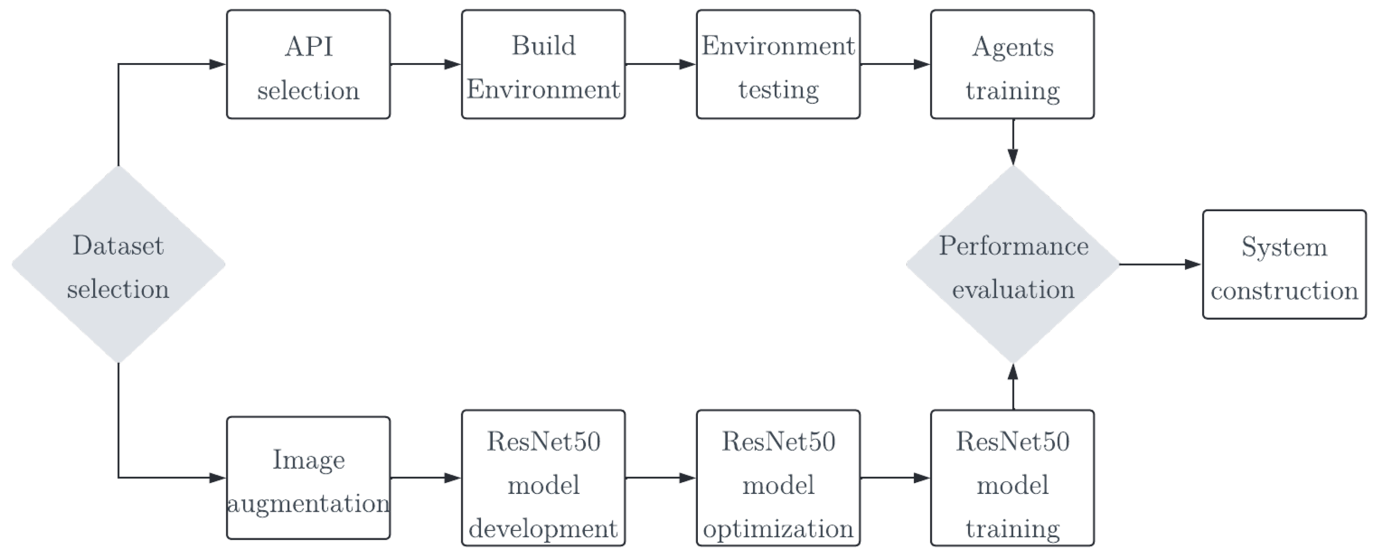
Figure 1.
Conceptualization of the proposed approach.
Figure 1.
Conceptualization of the proposed approach.
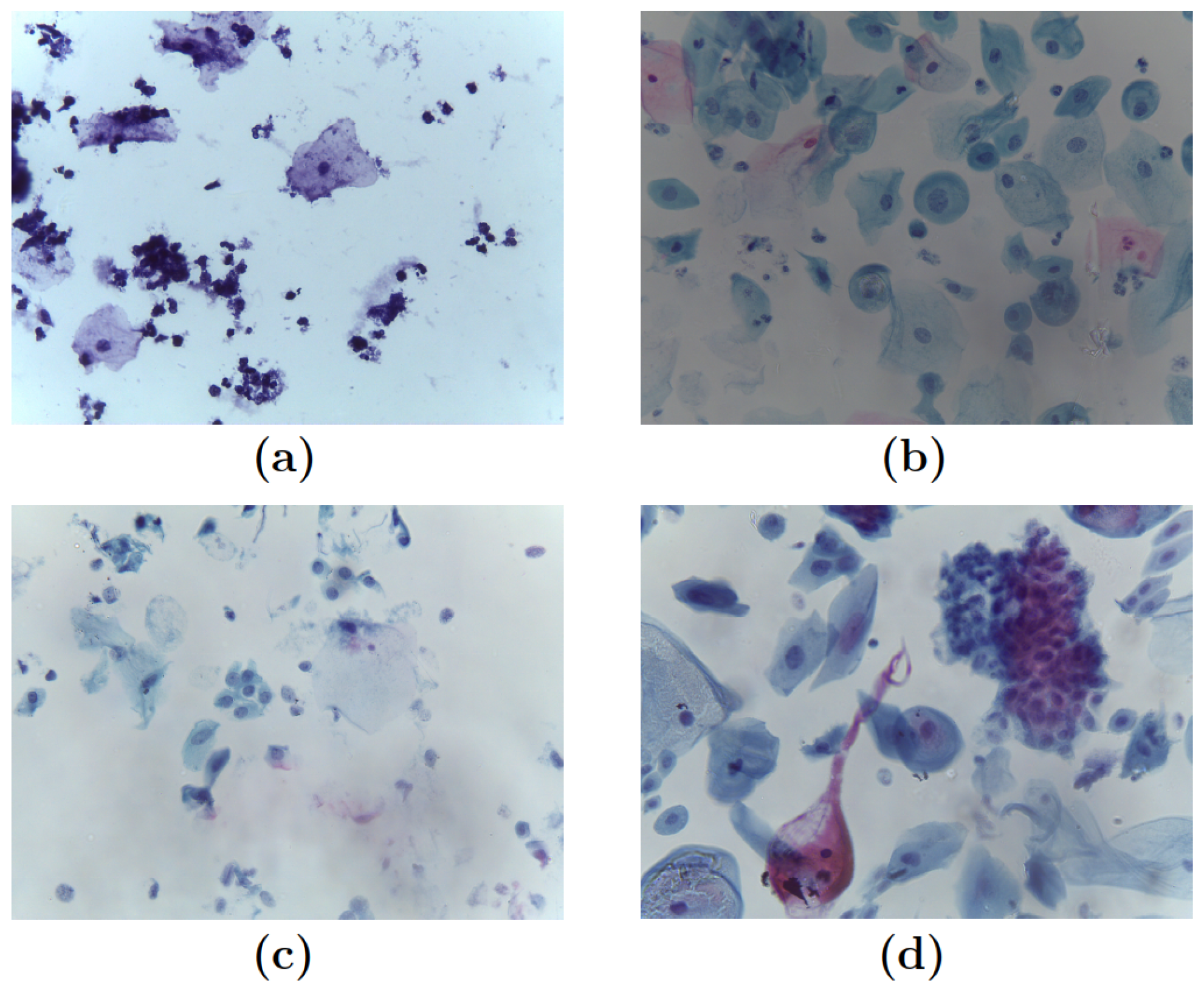
Figure 2.
Pap smear samples: (a) Negative for intraepithelial lesion or malignancy (NILM). (b) Low-grade intraepithelial lesions (LSIL). (c) High-grade intraepithelial lesions (HSIL). (d) Squamous cell carcinoma (SCC).
Figure 2.
Pap smear samples: (a) Negative for intraepithelial lesion or malignancy (NILM). (b) Low-grade intraepithelial lesions (LSIL). (c) High-grade intraepithelial lesions (HSIL). (d) Squamous cell carcinoma (SCC).
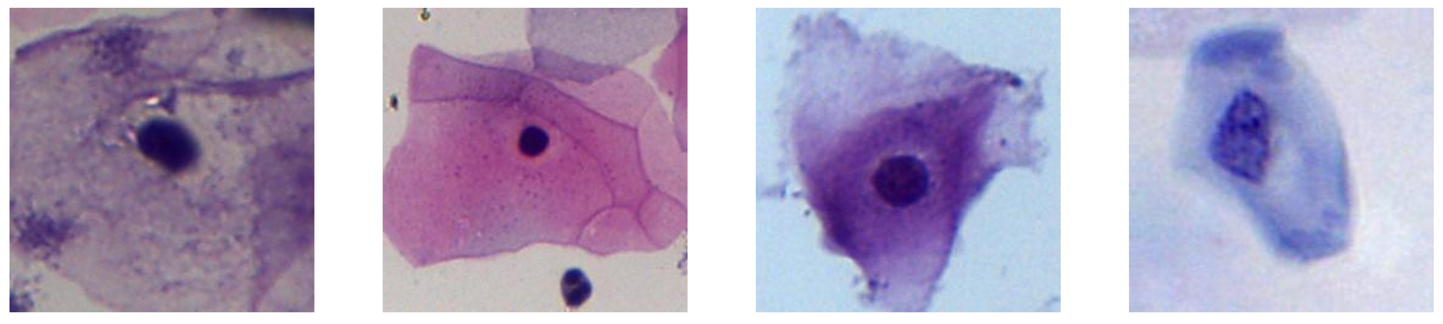
Figure 3.
Examples of extracted “Cells”.
Figure 3.
Examples of extracted “Cells”.
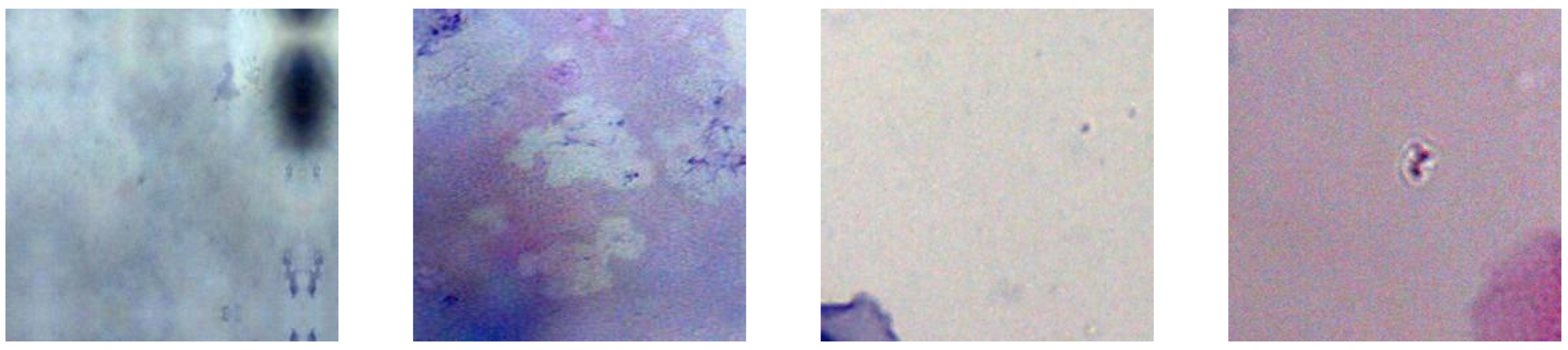
Figure 4.
Examples of extracted “No cells”.
Figure 4.
Examples of extracted “No cells”.
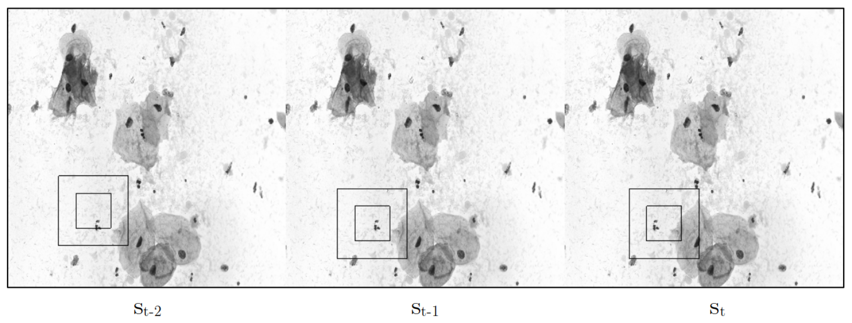
Figure 5.
The figure illustrates a stack of frames, visually representing the environment in which an agent interacts. The agent is characterized by two black squares and the motion it exhibits within the frames.
Figure 5.
The figure illustrates a stack of frames, visually representing the environment in which an agent interacts. The agent is characterized by two black squares and the motion it exhibits within the frames.
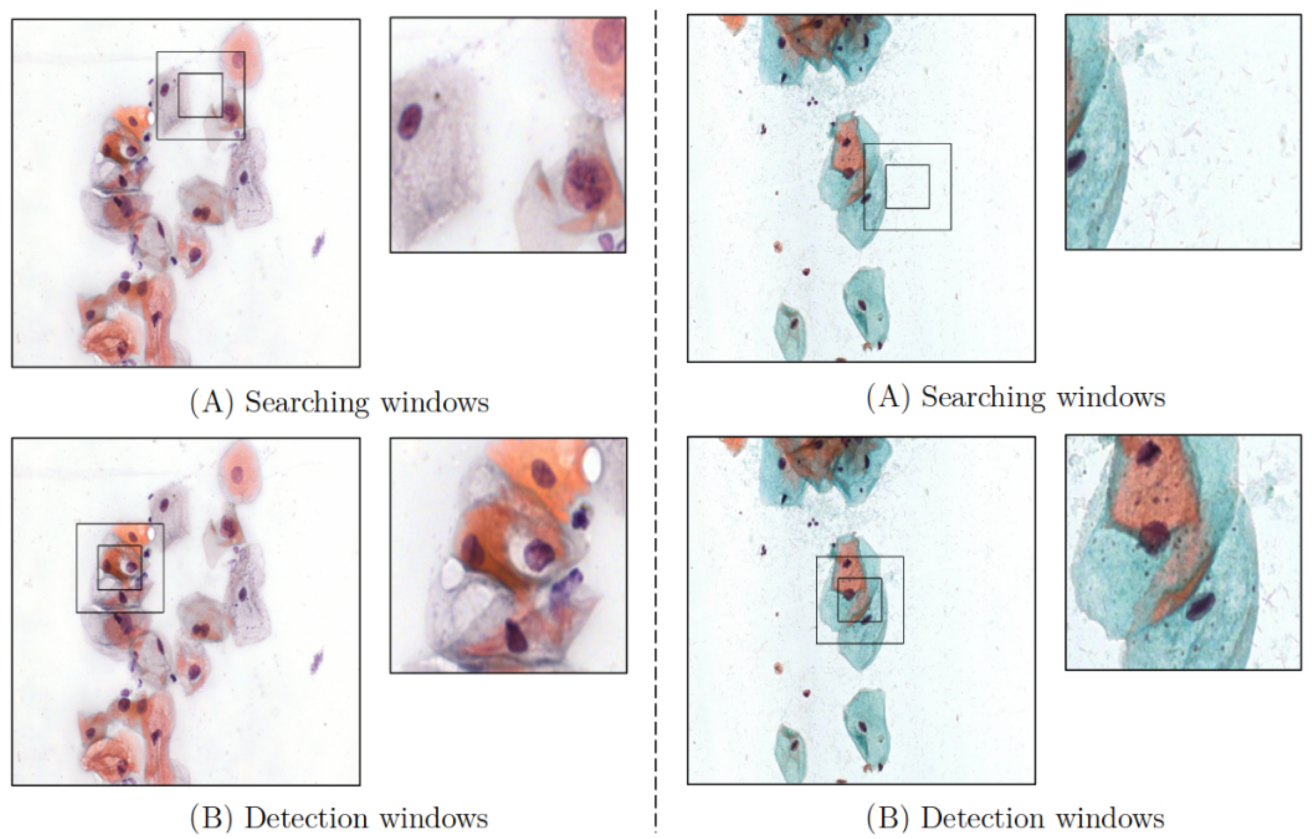
Figure 6.
Graphical representation of two environments. (A) It is the environment where the agent searches for cells, and the captured image by the ROI is displayed in the right window. (B) The cells that have been detected.
Figure 6.
Graphical representation of two environments. (A) It is the environment where the agent searches for cells, and the captured image by the ROI is displayed in the right window. (B) The cells that have been detected.
Figure 7.
A visual depiction of how data moves through the CNN.
Figure 7.
A visual depiction of how data moves through the CNN.
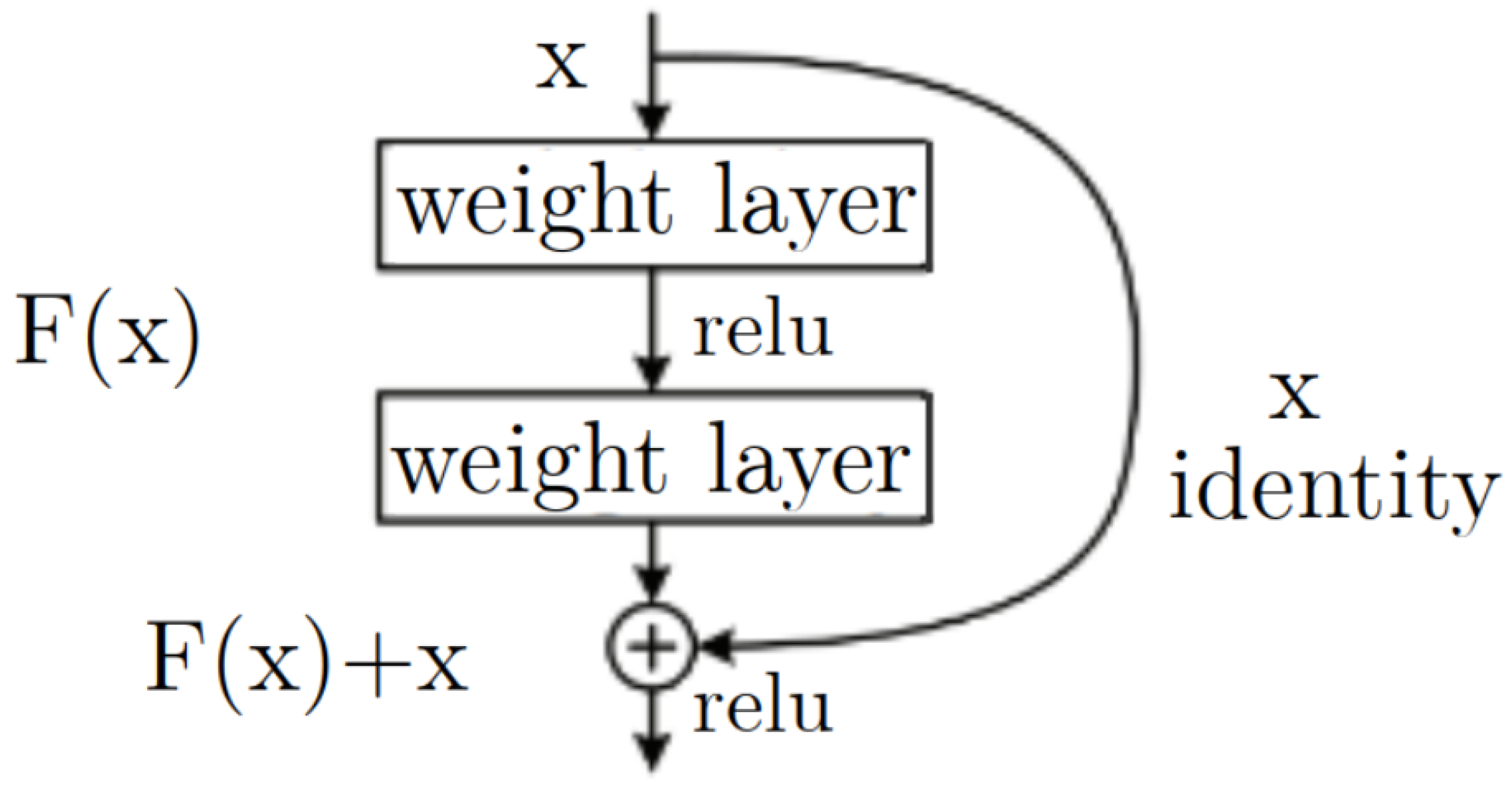
Figure 8.
Residual block architecture of ResNet model.
Figure 8.
Residual block architecture of ResNet model.
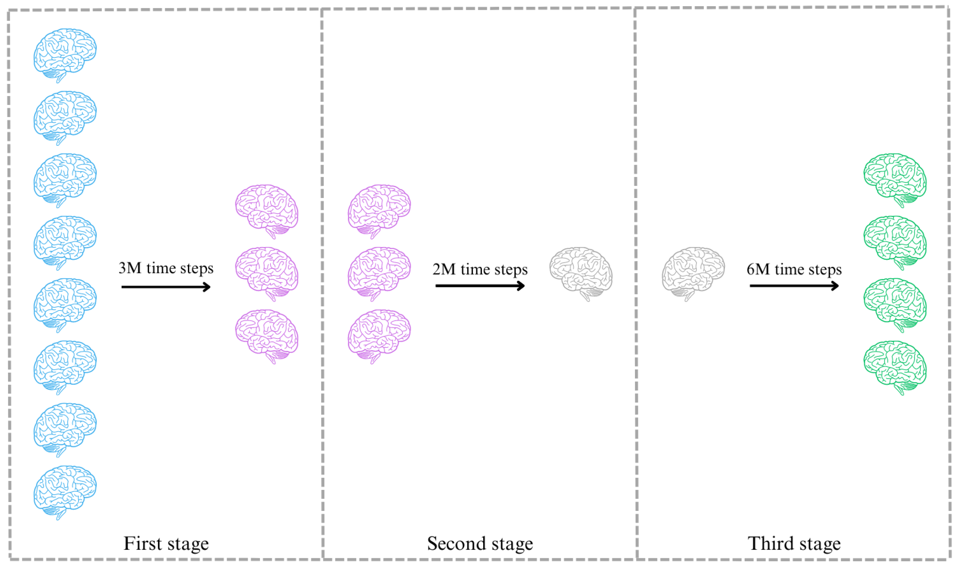
Figure 9.
Graphic representation of the stages during the training process.
Figure 9.
Graphic representation of the stages during the training process.
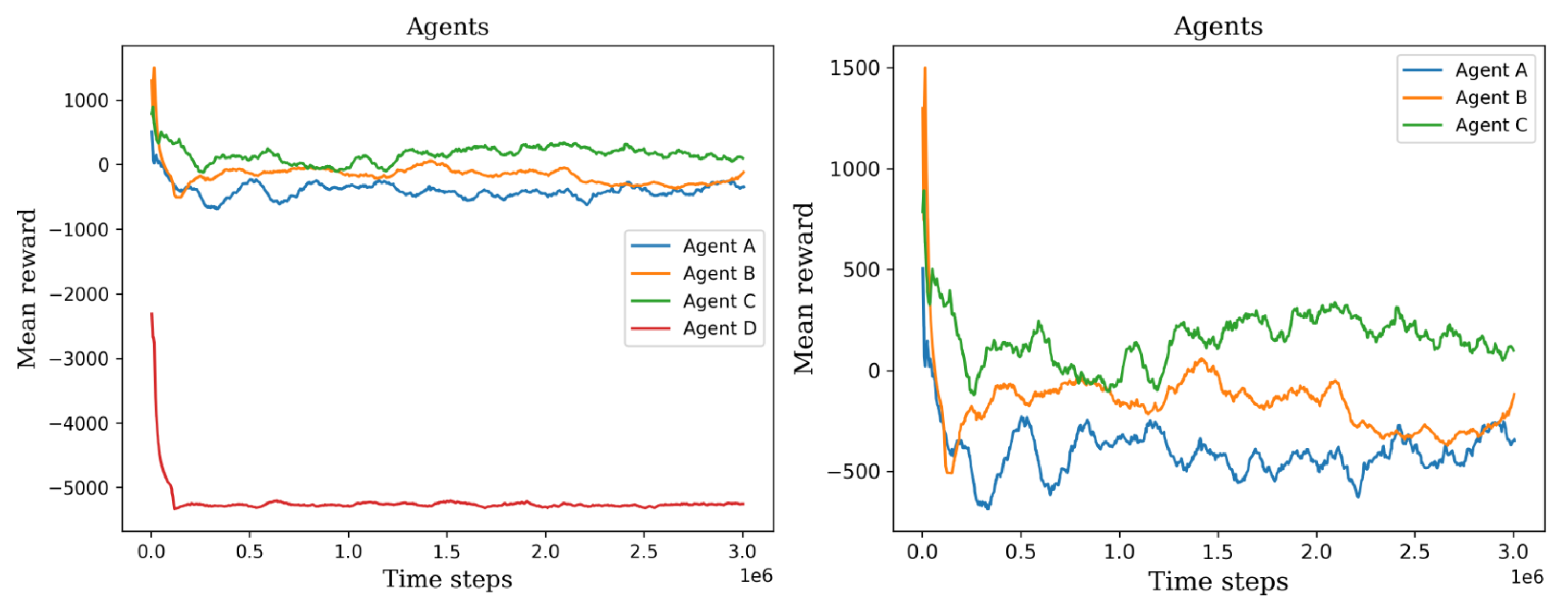
Figure 10.
The left plot shows all the first set of agents’ mean rewards, permitting the ability to visually compare their training process. The right plot shows only three agents, agent D was not considered because it has the lowest values.
Figure 10.
The left plot shows all the first set of agents’ mean rewards, permitting the ability to visually compare their training process. The right plot shows only three agents, agent D was not considered because it has the lowest values.
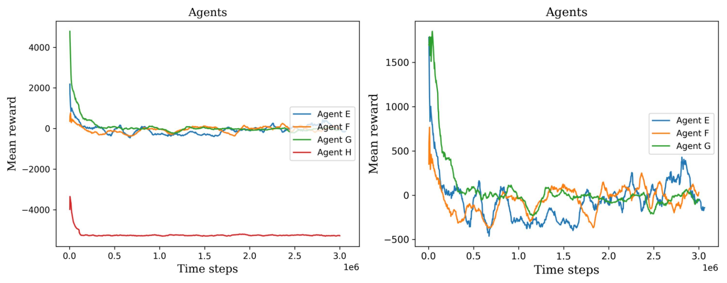
Figure 11.
The left plot shows all the second set of agents’ scores, permitting the ability to visually compare their training process. The right plot shows only three agents, agent H was not considered because it has the lowest values.
Figure 11.
The left plot shows all the second set of agents’ scores, permitting the ability to visually compare their training process. The right plot shows only three agents, agent H was not considered because it has the lowest values.
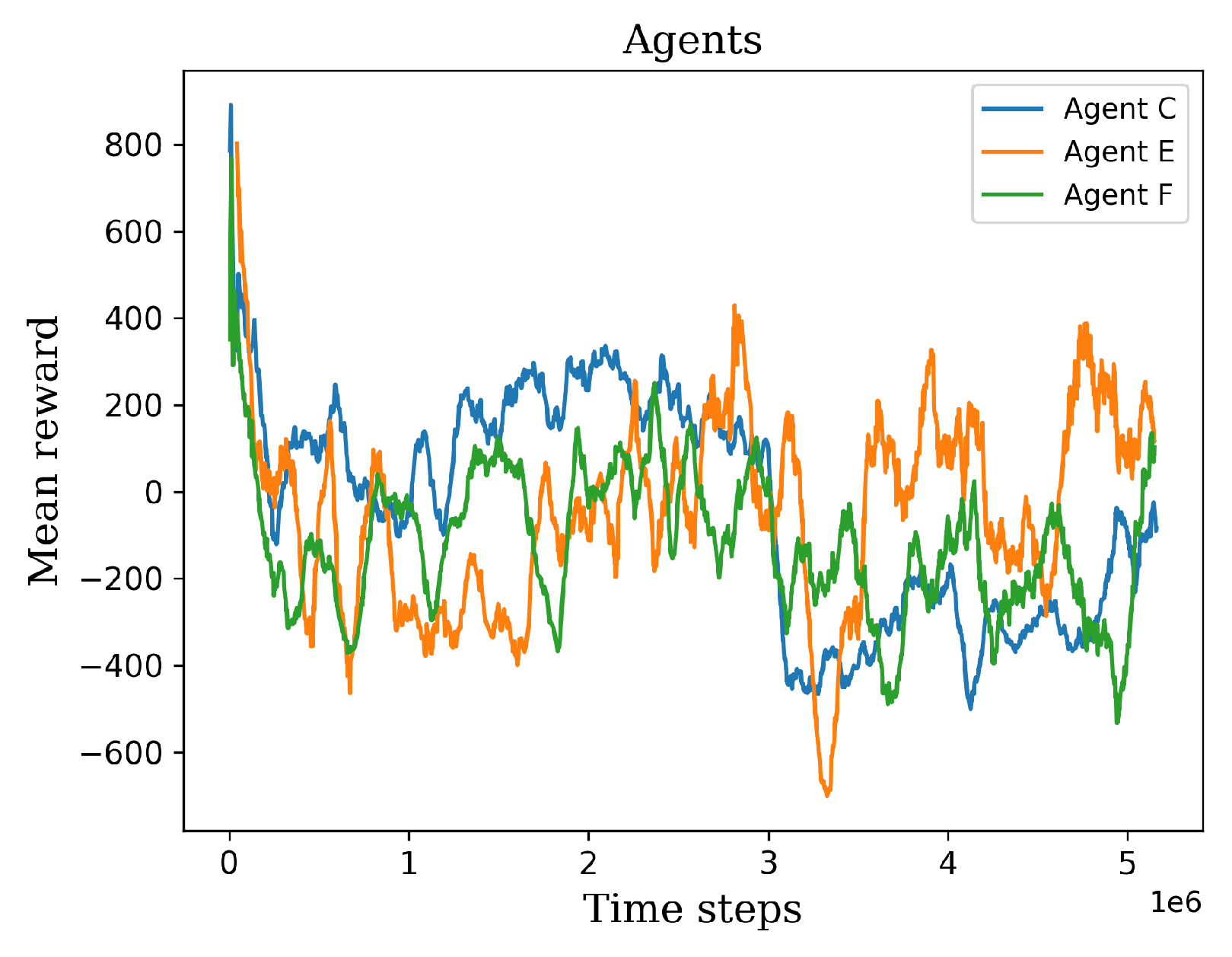
Figure 12.
The graph shows the retraining results of the agents C, E, and F.
Figure 12.
The graph shows the retraining results of the agents C, E, and F.
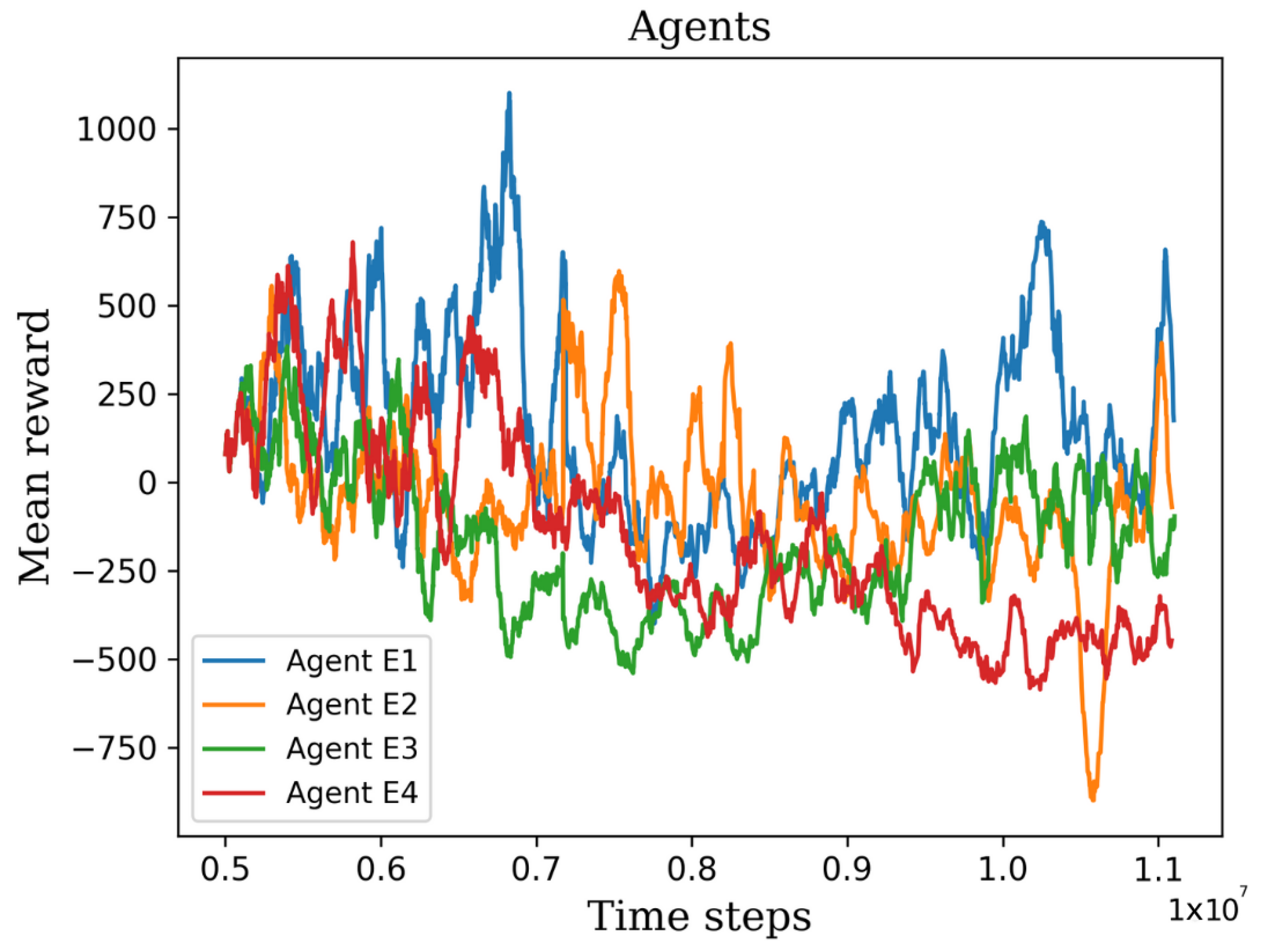
Figure 13.
The graph shows the retraining results of the four extensively trained agents.
Figure 13.
The graph shows the retraining results of the four extensively trained agents.
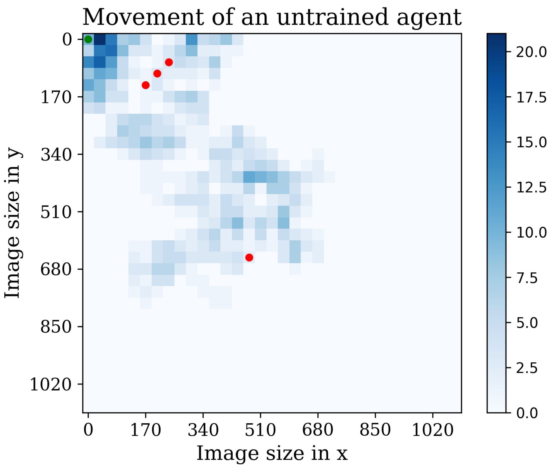
Figure 14.
The figure illustrates the behavior of an untrained agent. Red dots represent discovered cells, while the blue bar indicates repetitive visits to the same position.
Figure 14.
The figure illustrates the behavior of an untrained agent. Red dots represent discovered cells, while the blue bar indicates repetitive visits to the same position.
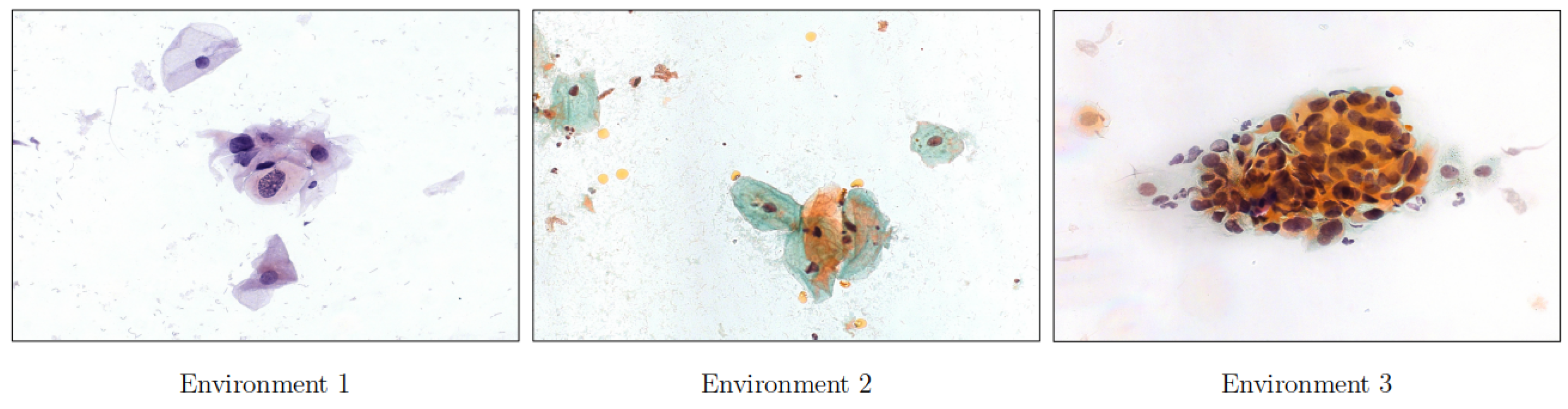
Figure 15.
The figure shows three distinct environments utilized for testing the agents during the second and third stages of experiments.
Figure 15.
The figure shows three distinct environments utilized for testing the agents during the second and third stages of experiments.
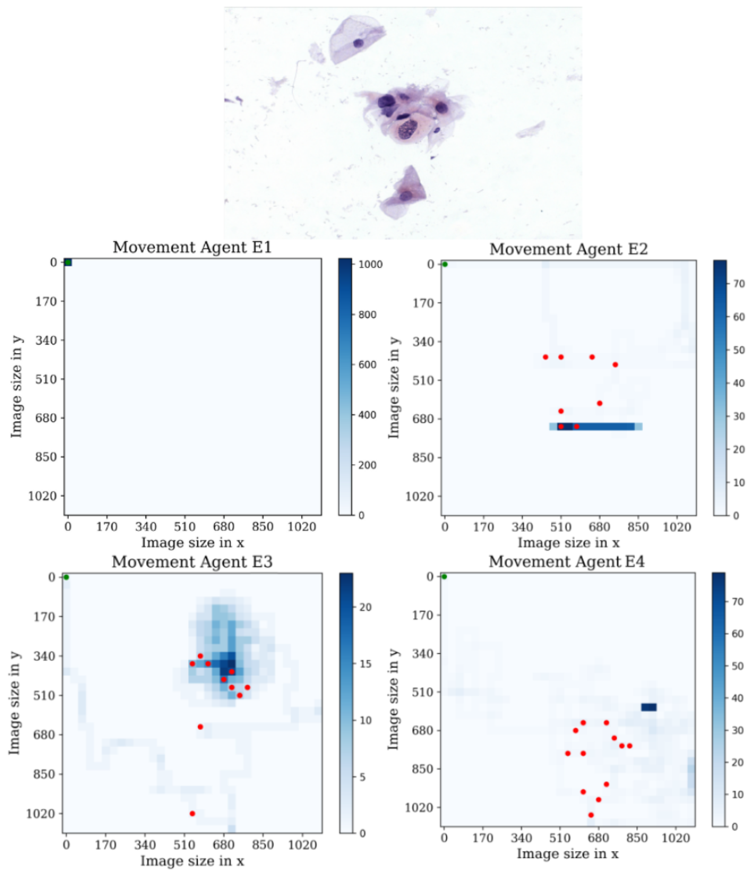
Figure 16.
Tracking results of the agents E1, E2, E3, and E4 from the last stage in the first environment.
Figure 16.
Tracking results of the agents E1, E2, E3, and E4 from the last stage in the first environment.
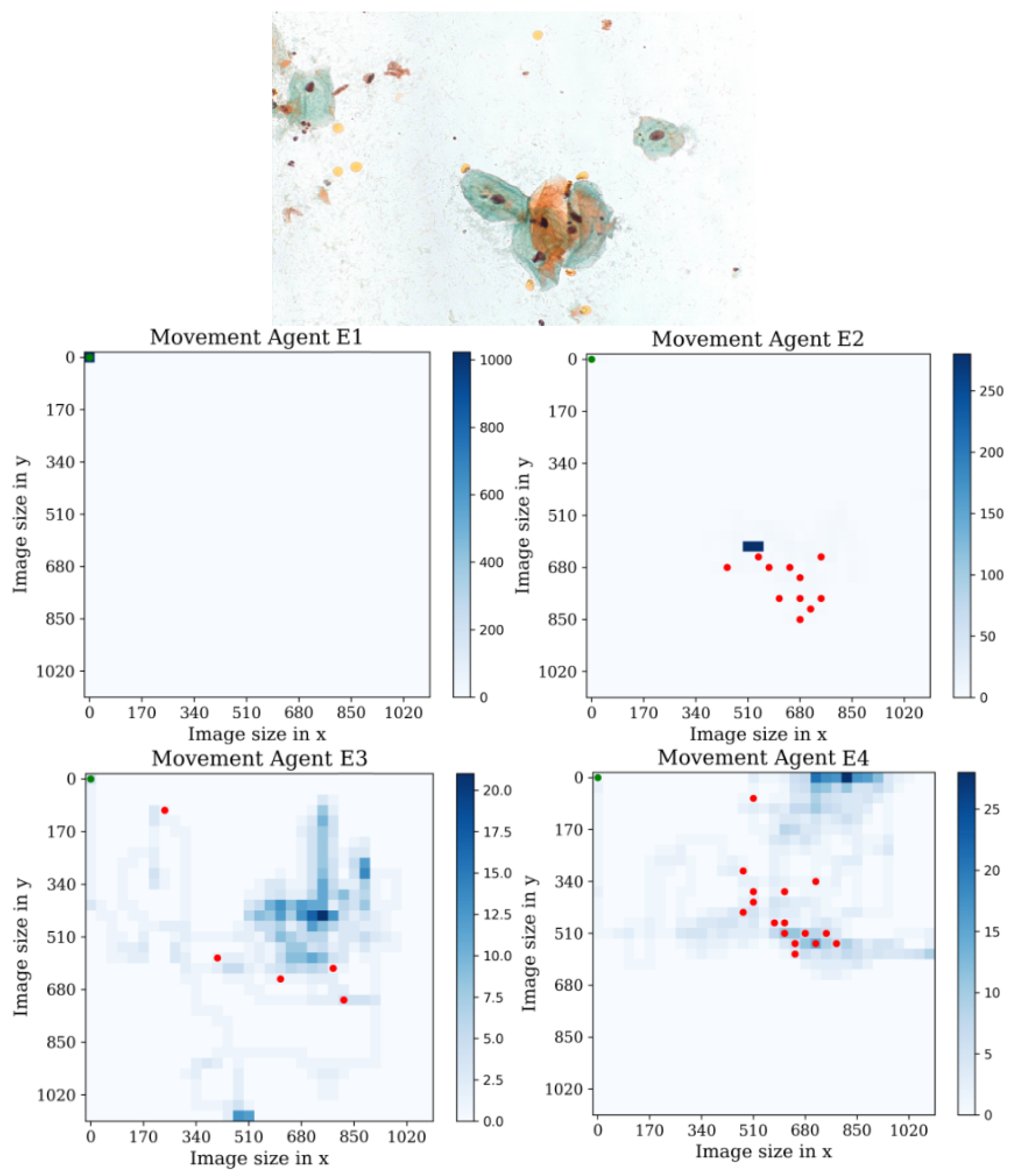
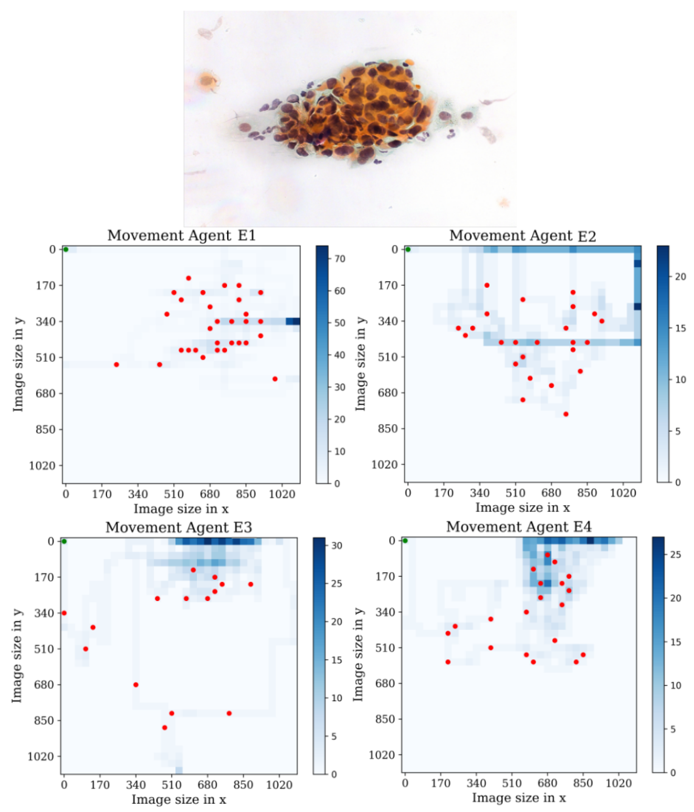
Figure 17.
Tracking results of the agents E1, E2, E3, and E4 from the last stage in the second environment.
Figure 17.
Tracking results of the agents E1, E2, E3, and E4 from the last stage in the second environment.
Figure 18.
Tracking results of the agents E1, E2, E3, and E4 from the last stage in the third environment.
Figure 18.
Tracking results of the agents E1, E2, E3, and E4 from the last stage in the third environment.
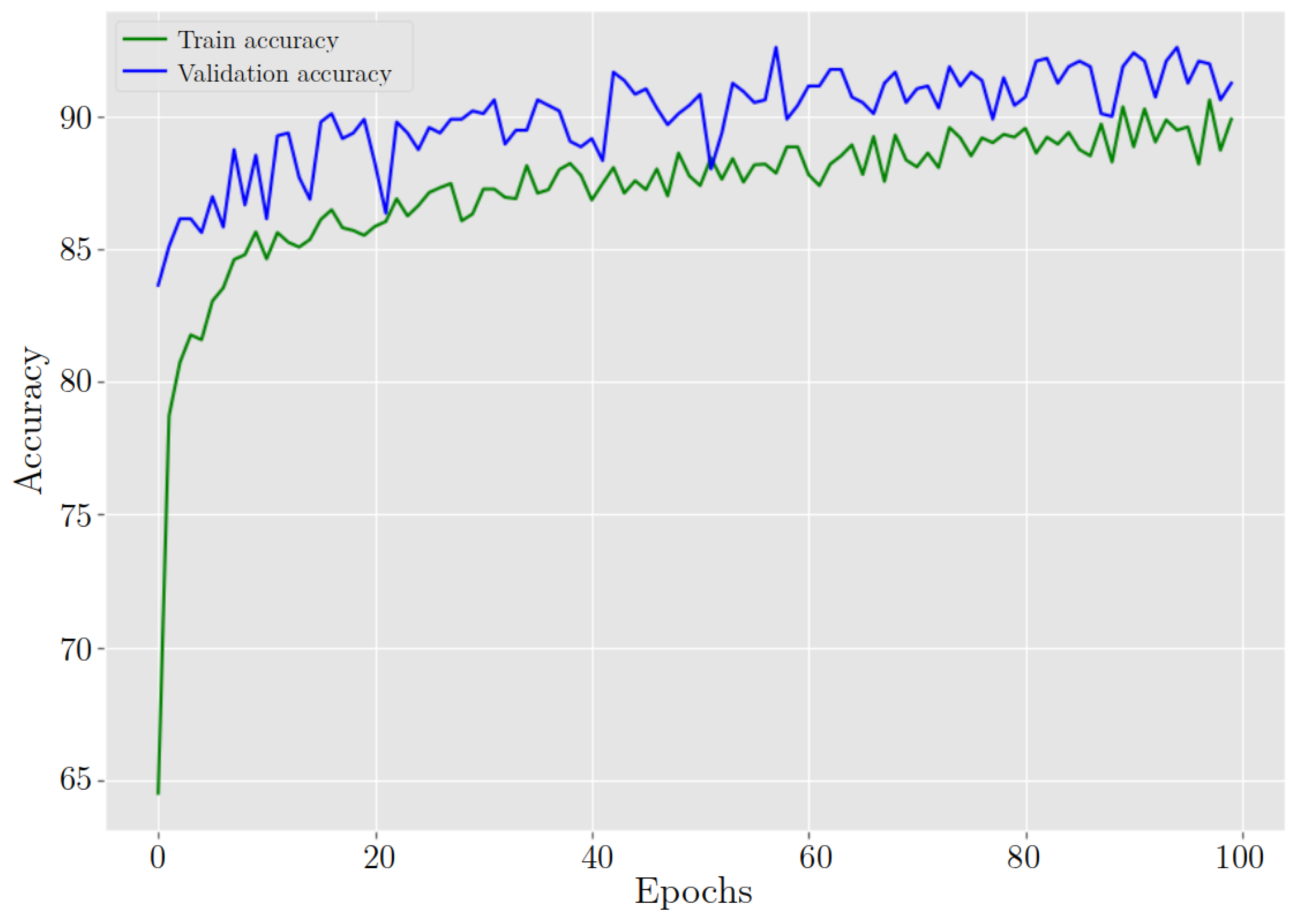
Figure 19.
ResNet-50 behavior in training and validation accuracy during 100 epochs.
Figure 19.
ResNet-50 behavior in training and validation accuracy during 100 epochs.
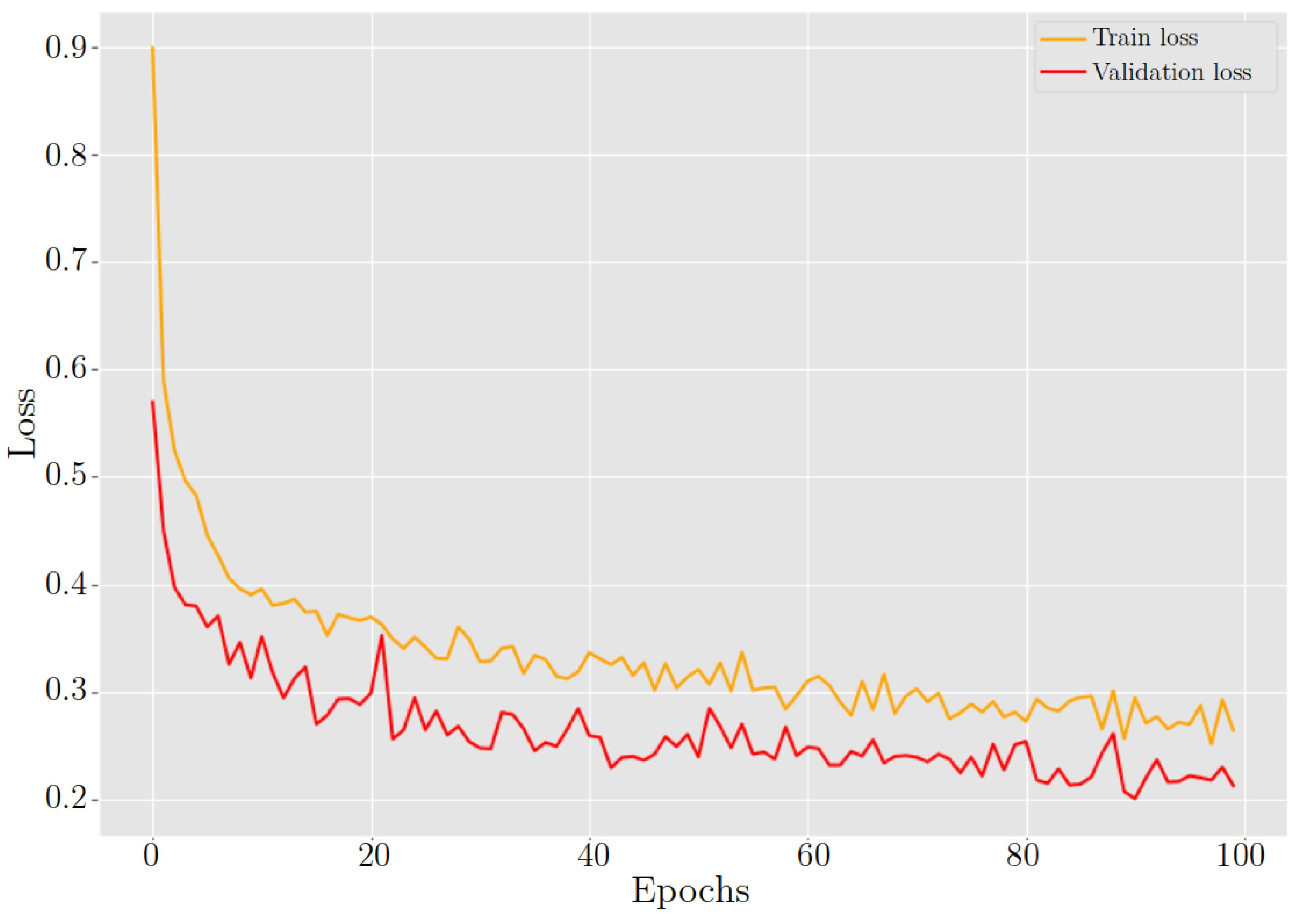
Figure 20.
ResNet-50 behavior in training and validation loss during 100 epochs.
Figure 20.
ResNet-50 behavior in training and validation loss during 100 epochs.
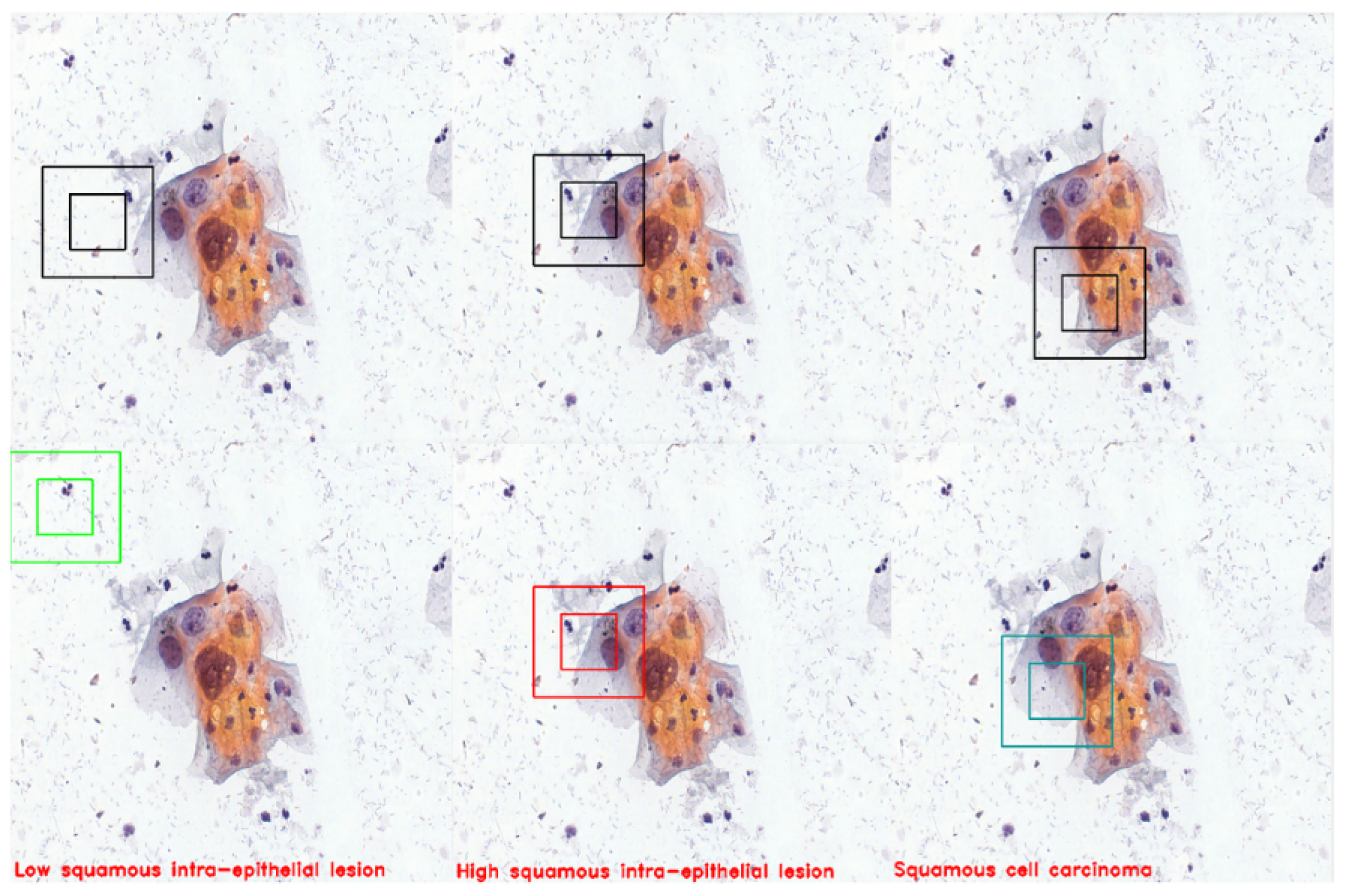
Figure 21.
The figure demonstrates three instances in which the agent successfully detects cells and accurately classifies them. The agent detected LSHL, HSIL, and SCC cells.
Figure 21.
The figure demonstrates three instances in which the agent successfully detects cells and accurately classifies them. The agent detected LSHL, HSIL, and SCC cells.
Table 1.
The actions are numbered from 1 to 4, with each number representing a specific direction. The environment interprets these numbers to facilitate the movement of the ROI.
Table 1.
The actions are numbered from 1 to 4, with each number representing a specific direction. The environment interprets these numbers to facilitate the movement of the ROI.
| Actions Number | Action |
|---|
| 1 | Right |
| 2 | Left |
| 3 | Up |
| 4 | Down |
Table 2.
Brief description of the agents.
Table 2.
Brief description of the agents.
| Agents | Description |
|---|
| A, E | Using the reward signal without changes. |
| B, F | No penalty for detecting the same cell multiple times |
| C, G | No penalty while searching for a cell |
| D, H | High penalty while searching for a cell, |
Table 3.
The hyperparameters included in the PPO Stable Baselines 3 implementation, with descriptions and values. The symbol following a hyperparameter name refers to the coefficient.
Table 3.
The hyperparameters included in the PPO Stable Baselines 3 implementation, with descriptions and values. The symbol following a hyperparameter name refers to the coefficient.
| Hyperparameters | Values | Description |
|---|
| learning_rate | | Progress remaining, which ranges from 1 to 0. |
| n_steps | 512; 1024 | Steps per parameters update. |
| batch_size | 128 | Images processed by the network at once |
| n_epochs | 10 | Updates for the policy using the same trajectory |
| gamma | | Discount factor |
| gae_lambda | | Bias vs. variance trade-off |
| clip_range | | Range of clipping |
| vf_coef | | Value function coefficient |
| ent_coef | | Entropy coefficient |
| max_grad_norm | | Clips gradient if it becomes too large |
Table 4.
Summary of metrics obtained with ResNet50 by category.
Table 4.
Summary of metrics obtained with ResNet50 by category.
| Categories | Precision | Recall | F1-Score | Support |
|---|
| NILM | 1.00 | 0.97 | 0.98 | 200 |
| LSIL | 0.94 | 0.92 | 0.93 | 200 |
| HSIL | 0.78 | 0.92 | 0.84 | 200 |
| SCC | 0.91 | 0.86 | 0.85 | 200 |
Table 5.
Comparison with other studies ordered by accuracy.
Table 5.
Comparison with other studies ordered by accuracy.
| AI Methods | Accuracy | Classes |
|---|
| ResNet50V2* [19] | 0.97 | 4 |
| ResNet101V2* [19] | 0.95 | 4 |
| ResNet50 | 0.91 | 4 |
| ResNetXt29_2*64d [20] | 0.91 | 10 |
| ResNetXt29_4*64d [20] | 0.91 | 10 |


